Identification of opposites and intermediates by eye and by hand

(1)

Contents lists available atScienceDirect

Acta Psychologica

journal homepage:www.elsevier.com/locate/actpsy

Identi

ﬁcation of opposites and intermediates by eye and by hand

Ivana Bianchi

a,⁎

, Carita Paradis

b

, Roberto Burro

c

, Joost van de Weijer

b

, Marcus Nyström

d

,

Ugo Savardi

c

a_{Department of Humanities, (section Philosophy and Human Sciences), University of Macerata, via Garibaldi 20, 62100 Macerata, (Italy)} b_{Centre for Languages and Literature, Lund University, Box 201, SE-221 00 Lund, (Sweden)}

c_{Department of Human Sciences, University of Verona, Lungadige Porta Vittoria 17, 37129 Verona, (Italy)} d_{Humanities Laboratory, Lund University, Box 201, SE-221 00 Lund, (Sweden)}

A R T I C L E I N F O

Keywords: Opposites Intermediates Spatial dimensions Points Ranges Perceptual grounding

A B S T R A C T

In this eye-tracking and drawing study, we investigate the perceptual grounding of different types of spatial dimensions such asDENSE–SPARSEandTOP–BOTTOM, focusing both on the participants' experiences of the opposite regions, e.g., O1:DENSE; O2:SPARSE, and the region that is experienced as intermediate, e.g., INT:NEITHER DENSE NOR SPARSE. Six spatial dimensions expected to have three different perceptual structures in terms of the point and range nature of O1, INT and O2 were analysed. Presented with images, the participants were instructed to identify each region (O1, INT, O2),first by looking at the region, and then circumscribing it using the computer mouse. We measured the eye movements, identification times and various characteristics of the drawings such as the relative size of the three regions, overlaps and gaps. Three main results emerged. Firstly, generally speaking, intermediate regions were not different from the poles on any of the indicators: overall identification times, number offixations, and locations. Some differences emerged with regard to the duration of fixations for point INTs and the number offixations for range INTs between two range poles (O1, O2). Secondly, the analyses of the fixation locations showed that the poles support the identification of the intermediate region as much as the intermediate region supports the identification of the poles. Finally, the relative size of the three areas selected in the drawing task were consistent with the classification of the regions as points or ranges. The analyses of the gaps and the overlaps between the three areas showed that the intermediate is neither O1 nor O2, but an entity in its own right.

1. Introduction

A puzzling observation that has received a fair amount of attention in science was Galilei's discovery of the isochronous motion of the pendulum. When observing the swinging motion of the chandelier in Pisa Cathedral, Galilei was surprised to note that it appeared to swing slower than he expected it to swing. Subsequent and more recent stu-dies in theﬁeld of naïve physics have demonstrated that there is in fact a range of oscillation speed that human observers perceive as natural, i.e., as neither too fast nor too slow (Bozzi, 1958–59; Bressanelli, Bianchi, Burro, & Savardi, 2008; Frick, Huber, Reips, & Krist, 2005; Pittenger, 1990). Galilei's observation is interesting for two reasons. Firstly, it points to the fact that human beings seem to have an intuitive feeling for natural movements of physical phenomena with respect to speed. Secondly, it suggests that humans organize their experiences both in relation to the poles and to the intermediate region. In the case of the chandelier in Pisa, the dimension isSPEEDand the opposing poles

areFASTandSLOW. In the middle, there is an intermediate range per-ceived to be the natural speed.

Now, a natural state of perceived intermediateness is by no means restricted to Galilei's observations in Pisa, but applies to much more mundane situations. Several times every day, we are engaged in si-tuations that have to do with the identiﬁcation of opposites and inter-mediates. For instance, there are places in our town that we perceive to be near the house where we live, others that we perceive to be far away, and still others that we perceive to be neither near nor far away. The human ability to perceive intermediate regions is by no means re-stricted to spatial dimensions, but applies in a similar way to various domains such as temperature, smell, touch, taste, and sound. For in-stance, when we adjust the volume of the radio or the temperature of the air-conditioner, we usually adjust them so that they are neither too high nor too low but at an intermediate level.

In spite of the fundamental role of intermediateness for nearly all doings in our daily lives, there is hardly any research at all on

http://dx.doi.org/10.1016/j.actpsy.2017.08.011

Received 5 July 2016; Received in revised form 29 May 2017; Accepted 29 August 2017 ⁎_{Corresponding author.}

E-mail addresses:ivana.bianchi@unimc.it(I. Bianchi),carita.paradis@englund.lu.se(C. Paradis),roberto.burro@univr.it(R. Burro),joost.van_de_weijer@ling.lu.se(J. van de Weijer),

marcus.nystrom@humlab.lu.se(M. Nyström),ugo.savardi@univr.it(U. Savardi).

(2)

intermediate states in psychology or cognitive science. This study aims to startﬁlling that gap by speciﬁcally focusing on the nature of inter-mediateness in perception and cognition. Using pictures, we explore the grounding of participants' perception of the intermediate region (INT) of spatial dimensions, namely the part of the dimension that is per-ceived as neither one nor the other of the opposite regions (O1, O2).

Dimensional contrast and binary opposition in language have been given a fair amount of attention (Fellbaum, 1995, 1998; Israel, 2004; Jones, Murphy, Paradis, & Willners, 2012; Ogden, 1932; Osgood & Richards, 1973; Paradis, Löhndorf, van de Weijer, & Willners, 2015; Paradis & Willners, 2011). Findings from those studies suggest that opposition is a salient, binary configurational construal along meaning dimensions (Paradis & Willners, 2011), and both behavioral and neurophysiological experiments have shown that opposing expressions (antonyms) along par-ticularly salient dimensions have strong priming effects on one another, both outside and within a specific context (van de Weijer, Paradis, Willners, & Lindgren, 2012, 2014). However, the intermediate region has so far been disregarded in these linguistic studies. The reason may be that there is a conspicuous lack of domain-specific words for intermediateness in many languages of the world. What language users do instead when they talk about intermediate properties is that they say that something is neither long nor short, neither small nor large. Speakers may use words such as middle, in between, half, or they may add degree modifiers such as fairly long or not short, which are expressive of a region that may coincide with INT, but is not INT proper since they take the perspective of one of the opposite properties, e.g., fairly long, fairly short, not long, not short (Paradis, 1997, 2001, 2008; Paradis & Willners, 2006, 2013). There are, in fact, a few ex-ceptions to this general observation of lack of domain specific words. For instance, along the dimension of temperature, there are expressions such as lukewarm, tepid (En), lau, lauwarm (Ge), tibio, templado (Sp), tiède (Fr), tiepido (It), ljum (Sw), haalea (Fi), and there is oblique, which refers to a state that is neither perpendicular nor parallel to a given line or a surface along a spatial dimension. Oblique is, however, more of a technical term than an expression used in everyday communication. Why some intermediates are lexicalized while others are not is an interesting question to pursue, but before we can do that, we need to determine whether intermediates are indeed real in the sense that they are experienced as spatial components of dimensions that do not coincide with either of the opposite spatial components. Should this be the case, future investigations of dimensions and meaning construals of opposing properties and their expressions in language will have to take a new look at the perceptual and conceptual underpinnings of intermediates.

1.1. Perceptual grounding of opposites and intermediates

While there is a fair number of studies on binary contrast, bound-aries and ranges in language and cognition based on the assumption that they are perceptually grounded (Paradis, 2008; Paradis & Willners, 2006, 2013; Paradis, Willners, & Jones, 2009), only two previous stu-dies have speciﬁcally addressed the question of whether what lies in between the poles is perceived as a gradient extension of the poles, rather than an experience speciﬁcally recognized as being neither one pole nor the other (Bianchi, Burro, Torquati, & Savardi, 2013; Bianchi, Savardi, & Kubovy, 2011). In these studies, the perceptual structure of 37 spatial dimensions, e.g., NEAR–FAR, NARROW–WIDE, HIGH–LOW, END– -BEGINNING,IN FRONT OF–BEHIND, in terms of three, and not two, components

was examined, namely the two opposite poles and the intermediate region. The extensions of the two poles and the intermediate regions were metrically deﬁned by the number of instances in proportion to the whole dimension that adults recognize as diﬀerent experiences of a property, for instanceSMALLNESS, the opposite property,LARGENESS, and the intermediate state,NEITHER LARGE NOR SMALL. The two poles and the

intermediate region were also topologically classiﬁed, either as points or ranges. For example, along the aperture dimension OPEN–CLOSED,

CLOSEDis a singular, unique state, a point, whereasOPENis a range, which

comprises various diﬀerent degrees ofOPENNESS, and it was shown that,

in most of the cases, the sum of the instances of the two poles did not

exhaust the entire dimension (Savardi, Bianchi, & Burro, 2009, pp. 287ff). These experiments resulted in three important findings of re-levance for the research presented in this article. Firstly, the partici-pants frequently identified intermediate experiences as neither one pole nor the other (INTs). This intermediate region sometimes consisted in a single experience, i.e., a point (P) property such as‘neither in front of nor behind’ (and therefore it has very limited extension within the whole dimension) or a range (R) such as‘neither the end nor the be-ginning’ or ‘neither near nor far away’ (and therefore it has a larger spatial extension within the dimension). Secondly, they showed that INTs do not necessarily occupy a pivotal position, but can be located closer to one or the other of the opposite poles. Thirdly, INTs were rated at the same speed as the opposite poles, which is afinding of particular importance for the study presented in this article because it suggests that the identification of INT does not involve an operation of double exclusion of the opposite poles as expressions such as neither–nor might lead one to think.

In this study, we make use of the abovefindings about the nature of points and ranges for opposites and intermediates as a springboard for the formulation of new research questions using two different observa-tional techniques: an online eye-tracking task and an offline, drawing task. In order to tap into the participants' perceptual experiences, images showing three spatial Dimension Types are included in the tasks. The component parts of the Dimension Types are O1–INT–O2, where Range–Range–Range (RRR) is represented by NEAR–FAR AWAY and DENSE–SPARSE, Point–Range–Point (PRP) byEND–BEGINNINGandTOP–BOTTOM,

and Range–Point–Range (RPR) byIN FRONT OF–BEHINDandABOVE–BELOW. The main questions are whether the intermediates are perceived in the same way as the opposite poles, and whether wefind additional evi-dence in support of their nature as points or ranges. More generally, the study is meant to be a contribution to the rather extensive literature in cognitive science and psychology on embodiment and situated cognition (e.g., Barsalou, 2010; Borghi & Cimatti, 2010; Gibbs, 2006; Lakoff & Johnson, 1999), to theories of semantics that make claims about the grounding of language and cognition in perception, and the-ories of semantics that see language, cognition and perception as com-municating vessels (Caballero & Paradis, 2015; Gärdenfors, 2014; Langacker, 1987; Paradis, 2015a; Talmy, 2000; Zwaan, 2004). By adding more experimental research on the perception of intermediates along various binary dimensions (by means of eye-tracking and new behavioral drawing data) to the relatively fewfindings in the literature, the results of this study contribute to stressing the need to rethink the modeling of opposites in terms of three rather than simply two com-ponents, i.e., the two opposite poles. Also, the results raise important questions about why only opposites, and not intermediates, are worthy of lexicalization in natural languages. Is the reason a matter of percep-tual salience, epistemic informativeness, priority in terms of ontogenetic development or something else? These questions cannot be answered based on the results of the present study, but if this study adds more experimental evidence of the direct perception of intermediates along dimensions, questions of this kind will arise as a natural consequence.

In the next section, we elaborate on the reasons for why we expect the perceptual system to be sensitive to the intermediate region, not only to the poles, along oppositional dimensions.

2. Intermediates and opposite poles

From work in philosophy, psychology, cognitive science, and linguis-tics, we know that our perception of space is anchored in our bodies (e.g., Barsalou, 1999, 2010; Beveridge & Pickering, 2013; Bianchi, Savardi, Burro, & Martelli, 2014; Borghi & Cimatti, 2010; Caballero & Paradis, 2015; Gibbs, 2006; Gibson, 1979; Howard & Templeton, 1966; Lakoﬀ & Johnson, 1980, 1999; Paradis, Hudson, & Magnusson, 2013; Varela, Thompson, & Rosch, 1991). We, as human beings, experience ourselves to be in the middle of space that opens up around us. We are neither at one nor the other of the extremes of the sagittal axis

(3)

(front–back), the coronal axis (right–left) or the gravitational axis (up–-down) but right in the middle. These dimensional contrasts and binary oppositions are important for how we view ourselves within and in rela-tion to space. They are not only crucial for our experience of the world, but also for how we think and reason, and consequently also for how mean-ings are construed in human communication through language (Chilton, 2014; Gärdenfors, 2014; Langacker, 1987; Paradis, 2005, 2015a; Talmy, 2000). The experience of a neither–nor region between the contrasts is part and parcel of this embodied spatial organization, i.e., a region which is neither front nor back, neither left nor right, or neither up nor down.

Furthermore, various indications have emerged from psychophysics and perceptual studies in variousfields showing that the human (and animal) perceptual system is sensitive to“the middle”. For instance, bisections tasks, where participants are asked to locate or identify the middle of something, are widely used in psychology. They are not considered cognitively de-manding, rather they are standard tasks used to diagnose hemispatial ne-glect (e.g.,Bonato, Priftis, Marenzi, & Zorzi, 2008; Ferber & Karnath, 2001) and homonymous hemianopia (e.g., Kerkhoff & Bucher, 2008; Schuett, Dauner, & Zihl, 2011). Furthermore, bisection tasks are commonly applied in order to study healthy people's perception in different sense modalities (e.g., Brooks, Della Sala, & Logie, 2011; Masin, 2008; Millar & Al–Attar, 2000; Ocklenburg, Hirnstein, Hausmann, & Lewald, 2010; Post, O'Malley, Yeh, & Bethel, 2006). They have also been used to study numerical cogni-tion (e.g.,De Hevia & Spelke, 2009; Gebuis & Gevers, 2011), the processing of temporal information (e.g., Mioni, Zakay, & Grondin, 2015), and the processing of written words (e.g., Arduino, Previtali, & Girelli, 2010; Fischer, 2000, 2004). These studies have demonstrated that what healthy participants identify is usually not the exact metric middle but their per-ception of a subjective middle (for a review, seeJewell & McCourt, 2000). From our point of view, this literature on bisection tasks is important be-cause it shows that the task is intuitive, straightforward, applies across different sensory modalities and is easily performed by participants of dif-ferent ages. In other words, the concept of intermediateness is clear to the participants; deviations are related to metric precision.

Another piece of evidence that the middle is a primitive concept comes from studies in animal and developmental psychology. It has been shown that chimpanzees are able to identify the middle element of a series of objects (Rohles & Devine, 1966, 1967), chickens can localize the central position of a close environment by learning geometric re-lationships such as the middle (Tommasi & Vallortigara, 2000; Tommasi, Vallortigara, & Zanforlin, 1997), and nutcrackers know how toﬁnd the point halfway between two landmarks at various distances (Kamil & Jones, 1997). Children start discriminating the middle ele-ment of a series of eleele-ments already at the age of three (Cox & Williams, 1993; Rohles, 1971; Welch, 1939). Between seven and ten years of age, they are able to generalize the concept across various types of experi-ences such as color, density, position, height, size and length (Graham, Jackson, Long, & Welch, 1944; Tsai & Chien, 1968). Additional evi-dence of the salience of intermediateness comes from areas of research that are concerned with the power of the center in analyses of direct perceptual organization (Arnheim, 1982; Metzger, 1954; Stucchi, Graci, Toneatto, & Scocchia, 2010; Stucchi, Scocchia, & Carlini, 2016). Fur-thermore, eye-tracking studies show that in displays containing two simple shapes, saccades tend to occur in a central place in between the two (for a review, see van der Stigchel & Nijboer, 2011; Vitu, 2008), while in displays showing isolated shapes or daily-life objects, the saccades typically fall toward the center of gravity of the object (Foulsham & Kingstone, 2013; He & Kowler, 1989; Henderson, 2003, 2007; Pajak & Nuthmann, 2013; Richards & Kaufman, 1969; van der Linden, Mathôt, & Vitu, 2015). It has also been shown that people are accurate in estimating the center of a mass of asymmetrical two-di-mensional shapes and asymmetrical three-dimensional objects (Baud–Bovy & Gentaz, 2004; Baud–Bovy & Soechting, 2001; Bingham & Muchisky, 1993; Cholewiak, Fleming, & Singh, 2015).

While intermediate properties have been regarded as a given in the various investigations mentioned so far, only two studies have

specifically addressed the definition of the structure of intermediates in relation to the poles, and they did it in terms of phenomenological psychophysics (Bianchi et al., 2013andBianchi et al., 2011; for a de-finition of phenomenological psychophysics, seeKubovy, 2002). Like these latter studies, the topic of the present work concerns the very nature of intermediates in relation to the poles.

3. The study

On the basis of previous work, using classiﬁcation tasks, and metric and topological descriptions (Bianchi et al., 2011; Bianchi et al., 2013), this study investigates participants' perceptions of the three compo-nents:ﬁrst opposite (O1) – intermediate region (INT) – second opposite (O2) of three spatial Dimension Types namely Range–Range–Range (RRR), Range–Point–Range (RPR) and Point–Range–Point (PRP) (see Table 1). Two main goals are at the center of the present study, namely

Table 1

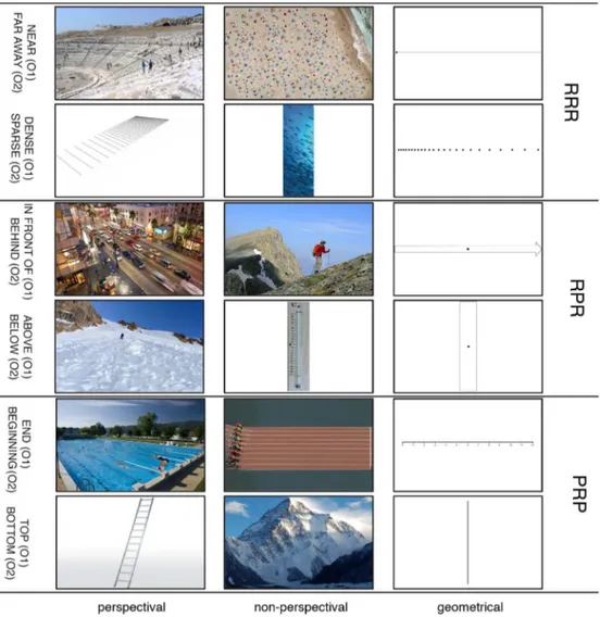
The stimuli used in the study. The Dimension Type is in capital letters from one pole through the intermediate region to the opposite pole in terms of their structural conﬁg-uration (R = range; P = point).

Dimension Type (O1 INT O2)

Dimension Image Image type

RRR Near–far away Greek theatre Photograph

(perspectival) (Sw: nära–långt

borta)

Beach Photograph (not

perspectival) Point along a line Drawing Dense–sparse Lines pattern Photograph

(perspectival)

(Sw: tät–gles) Fish Photograph (not

perspectival) Square dots along

a line

Drawing

RPR In front of–behind Cars in a lane Photograph (perspectival) (Sw:

framför–bakom)

Climber Photograph (not perspectival) Point in a band

arrow

Drawing

Above– below Mountain trekker Photograph (perspectival) (Sw: ovanför–

nedanför)

Thermometer Photograph (not perspectival) Point inside a

vertical band

Drawing

PRP End–beginning Swimming-pool Photograph

(perspectival) (Sw: slut–början) Running race Photograph (not

perspectival)

Ruler Drawing

Top– bottom Ladder Photograph

(perspectival) (Sw: överst–

nederst)

Mountain Photograph (not perspectival) Vertical line Drawing

(4)

(i) to provide further evidence of the three component parts and their configurational structures in terms of points and ranges using a com-bination of online and offline techniques to determine the validity of the classification proposed inBianchi et al. (2011)andBianchi et al. (2013), and (ii) to determine whether intermediates are perceived as basic units in the same way as the opposite regions of the dimensions. In pursuit of our goals, we make the following predictions.

1. If intermediates are basic units of the spatial dimensions in the same way as opposite poles are, their identiﬁcation time will be the same as for the poles.

2. When asked to identify the intermediates, the participants will look at the poles approximately as often as they look at the intermediates when they are asked to identify the poles. In other words, the identiﬁcation of the poles is dependent on the identiﬁcation of the intermediates to the same extent as the other way around. 3. There will be little or no overlap between the units that the

parti-cipants perceive as the intermediates or the poles, and there will be little or no space in between the three Target areas.

4. If the classiﬁcation of intermediates and the opposite poles as points or ranges is correct, we expect participants to mark areas corre-sponding to ranges with a larger surface than areas correcorre-sponding to

points, i.e., this should happen for two poles in dimension type RPR, for the intermediate region in dimensions PRP, and for both the poles and the intermediate region in dimensions RRR.

3.1. Method

3.1.1. Material

Each of the three Dimension Types (RRR, RPR and PRP) were re-presented by two spatial Dimensions, each of which was displayed in three diﬀerent Images: two photographs (one perspectival, the other one not), and one non-perspectival drawing: all in all, 18 stimuli were used for the experiment (3 Dimension Types × 2 Dimensions × 3 Images), as shown inTable 1and inFig. 1. Two additional Images were used as training stimuli. All of them were 1680 pixels wide and 1050 pixels high, corresponding to the resolution of the computer screen.

3.1.2. Participants

Twenty-ﬁve participants took part in the experiment (12 men and 13 women, 20–40 years old). They were all students and staﬀ at the Centre for Languages and Literature at Lund University and speakers of Swedish with normal or corrected–to–normal vision, and they were

Fig. 1. The stimulus images (color pictures) used in the study.

(5)

naïve to the purpose of the study. The experiment was carried out in accordance with the declaration of Helsinki.

3.1.3. Apparatus

Eye movements were recorded at 120 Hz in a room equipped with 25 RED-m remote video-based eye-trackers from SensoMotoric Instruments (Teltow, Germany). Each eye-tracker unit consists of an eye-tracker con-trolled by a computer, running SMI iView RED-m (v. 3.2.20), a Dell P2210 22″ screen with a resolution of 1680 × 1050 pixels (475 × 300 mm, equivalent to approximately 43.2 × 28.1° of visual angle at the re-commended viewing distance 650 mm) and a refresh rate of 60 Hz, a standard keyboard and mouse. Stimuli were presented with Python and PsychoPy (v. 1.79.01,Peirce, 2009).

3.1.4. Procedure

The participants sat in front of the computer screen, with the height of their seat adjusted to have their eyes level with the middle of the screen. The eye-trackers were ﬁrst calibrated to an accuracy level higher than one degree of the visual angle in the horizontal and the vertical direction.

After the calibration, the 18 Images were shown for 2 s one at a time. This preview of the Images aimed to minimize differences in re-sponse times between the first presentation of each Image and the following two presentations due to the novelty of thefirst presentation. Then the instructions were displayed on the computer screen1:“In this experiment we are interested in your perception of different dimensions such as loud–soft, clear–blurred. You will see the 18 images again. Before each image, you will be instructed to look at a particular part of it. For instance, you will see a box, and you will be asked to look at the part that you perceive to be the top of the box or the bottom of the box. We are also interested in knowing which part of the box you perceive to be ‘neither the top nor the bottom’. The reason for this is that nei-ther–nor is not necessarily the same as either of the extreme parts, but something else. For instance, a sound can be loud or soft or neither loud nor soft, which is when we are happy with it and see no reason to increase or decrease the volume. Please, read the instructions before each picture very carefully. Then press the spacebar to continue. You will see a red cross. Look at it! Once you have done that, the image will appear on the screen. Look at the part you were instructed to look at. Press the spacebar when you are done, and then mark the same area with the mouse. If you think that the drawing you made with the mouse was not quite right, you can delete it using the‘d’ key and make a new outline. When you are done, press the spacebar again to continue”.

The experiment started with the two practice trials after which the participants were given the opportunity to ask questions in case something was unclear. Then the actual experiment started. The ex-periment was self-paced. Its duration ranged from 10 to 20 min.

Each stimulus was presented three times: once with the instruction to identify the region showing O1; a second time with the instruction to identify the region showing O2; and the third time to identify the region showing INT. In total, the experiment consisted of 18 × 3 = 54 trials. The order of the stimulus presentation (both images and target re-gions) was randomized across the participants, with the restriction that the same Image was never presented in sequence. When the task con-cerned INT, half of the instructions read“neither O1 nor O2”, and the other half“neither O2 nor O1”. This was done to prevent the anchoring of the responses of the intermediate region to be more toward one or the other side of the dimension depending on the order in which the two poles were mentioned in the instructions. Both expressions are perfectlyﬁne in Swedish. Unlike the English expression, neither–nor, the Swedish expression, varken–eller, includes no element that is associated with the negator (inte‘not’).

3.1.5. Experimental design and analysis

The experimental design was entirely within subjects. We studied two independent variables: the Dimension Type (RRR, RPR, PRP) and the Target (O1, INT, O2, nested in Dimension Type). The analyses fo-cused on the following dependent variables: time needed to identify the Target area (the interval between onset of the presentation of the sti-mulus on the screen and the key press which signaled the participant's decision to start drawing), the characteristics of the drawing area (ex-tension of the outlines indicating the Target areas, the amount of overlap and the size of the gaps between them), and the eye movements during the identiﬁcation of the Target area (number, location, and duration ofﬁxations).

We performed mixed effects regression analyses (Linear Mixed Models, LMM, or Generalized Linear Mixed Models, GLMM) on the dependent variables. Unless otherwise specified, the predictors (fixed effects) were Dimension Type (PRP, RPR, RRR) and Target (INT, O1 and O2). Responses to the individual Images and Dimensions were not of interest to our study. Therefore, Images (nested in Dimension), Dimensions (nested in Dimension Type) and Subjects were entered as random factors in all statistical analyses conducted throughout the paper. However, in order to make it possible to relate ourfindings to the literature that, contrary to us, has specifically investigated how the typicality of words interact with features of the objects being described (e.g., Carlson-Radvansky & Irwin, 1993; Carlsson-Radvansky & Logan Gordon, 1997), we have specified in parenthesis how much of the total variance of the response variable which was analysed by each GLMM or LMM was in fact due to the Images. The analyses were carried out in the statistical software program R 3.3.0, with the packages‘lme4’ (Bates, Maechler, Bolker, & Walker, 2015),‘car’ (Fox & Weisberg, 2011), ‘ef-fects’ (Fox, 2003). The outcomes of the LMM or GLMM models were analysed with ANOVA tables, and the p-values were estimated with the parametric bootstrap method using the package ‘afex’ (Singmann, Bolker, Westfall, & Aust, 2017). Bonferroni corrections were applied to post hoc comparisons with package‘lsmeans’ (Lenth, 2016). When the outcome to be analysed was a ratio variable, namely identification time in Section 3.2.1, minimum distance in Section 3.2.2.2 and fixation duration in Section 3.2.3.3, the normality assumption was checked using the qqnorm function and the shapiro-test (R's stats-package) be-fore performing GLMMs of the Gaussian family. In all these cases, data turned out to be normally distributed. For ease of interpretability, all effect plots presented in this paper, and also those referred to GLMMs, where a Poisson or binomial family was used, show the results on the original scales.

3.2. Results

In this section, we start by considering the time the participants spent to identify the Target regions (Section 3.2.1). We then analyze the extensions of the parts of the images that the participants selected with the mouse and their overlaps and gaps (Section 3.2.2). Finally, we focus on the eye movement data, in particular on the number ofﬁxations needed to identify the Target regions, on the location and duration of theﬁxations (Section 3.2.3).

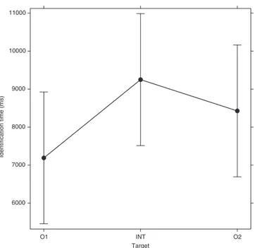
3.2.1. Identiﬁcation time

The analysis of identification time (GLMM Gaussian family) re-vealed a main effect of Target (χ2(2, N = 25) = 16.895, p < 0.0001), as shown inFig. 2. This was the only significant effect (a summary of the identification time per Dimension is reported inTable 2; effect size of Images: 8% of the total variance of Identification time). Post hoc comparisons showed that the difference in identification time between INT and O1 was significant (EST = 2066.997, SE = 505.162, t-ratio = 4.092, p < 0.0001), but not between INT and O2 (EST = 832.061, SE = 506.523, t-ratio = 1.643, p = 0.302). There-fore, these results indicate that, in general, there is no evidence that the identification of the intermediates was more time consuming than the 1_{The instructions to the participants were in Swedish.}

(6)

identification of the poles. The ordering of the opposing poles, named O1 and O2, was based on their extension, where O1 stands for the spatially smaller extension and O2 the larger one. In the light of this, the results suggest that the less extended pole was also the pole that was identified faster. We will return to the difference between O1 and O2 in thefinal discussion.

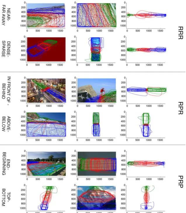
3.2.2. Outlines

Fig. 3shows the outlines drawn by all participants. We transformed the coordinates of the mouse movements by each participant2 into polygon areas within a Cartesian frame of reference using the R

packages ‘PBSmapping’ (Tanimura, Kuroiwa, & Mizota, 2006) and ‘splancs’ (Bivand & Gebhardt, 2000), and then determined the relative sizes of these areas, the distance between them, and the degree of overlap.

3.2.2.1. Proportional extension of the target areas. The proportional extension or relative size of the three polygons was determined as the size of each individual polygon divided by the total area of the three polygons. We considered the proportional extension of each area, rather than the absolute size, because the former is less dependent on the objects shown. For example, in the Images used in our study, the mountain and the swimming-pool covered a wider area of the screen than the thin line used for geometrical Images, and therefore the areas outlined in relation to the former were, in general, much bigger than the areas outlined in relation to the latter.

Table 2

Number ofﬁxations made and overall time needed for the identiﬁcation of the Target regions (O1, INT and O2) from the stimulus onset to pressing the spacebar to start drawing the outline of the Target region.

Dim. Type Dimension Image Identiﬁcation time (ms) Number ofﬁxations

Mean (SD) Mean (SD)

O1 INT O2 O1 INT O2 O1 INT O2 O1 INT O2

PRP End–beginning Ruler 7471.5 11,652.6 4708.2 6543.3 9860.9 4858.2 9.0 12.1 7.8 5.1 10.8 4.1

PRP End-–beginning Running race 7421.6 7550.1 5829.3 5198.5 6926.1 5357.9 9.9 10.1 8.4 7.5 6.6 4.9

PRP End-–beginning Swimming pool 8679.5 10,714.5 15,538.5 10,001 13,317.1 12,526.9 12.8 13.4 15.6 14.8 11.6 12.7

PRP Top–bottom Ladder 5210.0 8262.7 5506.7 4258.0 7280.1 5428.9 7.9 8.8 6.6 5.8 6.5 4.8

PRP Top–bottom Mountain 8589.6 7808.4 10,106.5 7573.8 7731.1 9632.4 9.6 12.9 16.2 9.2 10.3 15.4

PRP Top–bottom Vertical line 5323.5 8231.0 5745.0 3754.9 5449.3 5227.8 6.3 10.7 5.8 3.6 8.3 3.0

RPR Above–below Mountain trekker 9405.6 9648.9 10,641.4 5657.1 8814.5 11,327.3 12.8 13.5 16.0 7.7 9.6 9.7 RPR Above–below Point inside a vertical band 6761.6 8880.8 7087.9 6201.8 6996.7 7666.0 8.6 6.9 8.8 6.5 5.5 5.9

RPR Above–below Thermometer 7133.3 6932.4 8857.4 6313.8 6919.7 9540.8 10.4 7.1 7.9 6.7 5.7 5.1

RPR In front of–behind Cars in a lane 8657.8 7082.8 8227.9 8227.3 6552.9 7229.8 12.3 9.8 12.3 10.2 10.4 8.8

RPR In front of–behind Climber 5244.2 8271.4 9386.8 3649.7 7147.1 10,988.5 10.8 13.9 14.0 5.9 13.3 11.0

RPR In front of–behind Point in a band arrow 7493.5 9101.2 10,256.5 7433.8 10,121.0 9948.9 10.8 9.7 9.2 5.6 12.1 6.9

RRR Dense–sparse Fish 5620.6 8796.3 6798.3 5276.7 9831.2 7796.5 9.5 14.6 10.7 6.8 11.8 5.0

RRR Dense–sparse Lines pattern 8851.4 7032.1 5675.3 10,654.6 7113.8 4805.1 9.7 15.2 11.6 7.0 14.8 9.0

RRR Dense–sparse Square dots along a line 5749.1 9147.1 8222.5 6016.7 8618.6 6348.2 8.8 11.3 10.2 6.0 5.9 6.6

RRR Near–far away Beach 8393.8 10,200.5 6885.7 7115.3 7667.2 5515.0 12.2 17.9 13.8 16.4 12.8 10.6

RRR Near–far away Greek theatre 6198.2 14,499.2 10,494.9 4428.9 17,731.7 9870.1 13.5 19.8 15.6 9.8 20.4 14.0 RRR Near–far away Point along a line 6149.1 9840.6 8979.6 5348.8 9511.9 8149.7 7.4 14.5 11.5 6.4 9.3 7.9

Target Identification time (ms) 6000 7000 8000 9000 10000 11000 O1 INT O2

Fig. 2. Average identiﬁcation times (ms) of O1, INT and O2. Error bars represent 95% conﬁdence intervals.

2_{Due to a technical error in the recording of the mouse movements, the analyses of the} polygons were conducted on responses provided by 19 participants.

(7)

We expected the proportional extensions of point regions to be smaller than those of range regions. Thus, the poles of the PRP Dimension Type were expected to cover a relatively small area, while those of the RPR Dimension Type were expected to cover a relatively large area. In the Images showing the RRR Dimension Type, the dif-ference between the extensions of the three areas was expected to be smaller.

A GLMM (binomial family) was performed on the proportional ex-tensions. Target region (χ2(2, N = 20) = 5.264e + 06, p < 0.0001) and Dimension Type (χ2(2, N = 20) = 205.2, p < 0.0001) were sig-niﬁcant, as well as their interaction (χ2(4, N = 20) = 1.237e + 07,

p < 0.0001; effect size of Images: 16% of the total variance of the Proportional extension response variable). The interaction indicates that the average extensions of the three areas depended on the Dimension Type. For PRP Dimension Type (left panel ofFig. 4), the INTs covered around 50% of the total extension of the Dimension, while the two poles were significantly smaller, in between 20% and 30% of the total extensions each. Post hoc comparisons indicated that the INT was significantly larger than O1 (EST = 1.529, SE = 0.0005, z-ratio = 2661.504, p < 0.0001), and than O2 (EST = 0.554, SE = 0.0004, z-ratio = 1270.836, p < 0.0001).

Dimension Type RPR (see the middle panel of Fig. 4) had an

Fig. 3. Drawings made by all participants as corresponding to the three Target Regions: O1 (green), INT (red) and O2 (blue). (For interpretation of the references to color in thisﬁgure legend, the reader is referred to the web version of this article.)

(8)

opposite structure, with a small intermediate region (less than 15%) and the two poles covering the remaining 85% of the dimension. The diﬀerence between the intermediates and O1 was signiﬁcant (EST =−1.431, SE = 0.0007, z-ratio = −1923.678, p < 0.0001) and also O2 (EST =−2.075, SE = 0.0007, z-ratio =−2909.59, p < 0.0001).

For RRR Dimension Type (right panel ofFig. 4), the regions covered between 20% and 40% of the total dimension with the intermediate region having an extension signiﬁcantly larger than O1 (EST = 0.348, SE = 0.0004, z-ratio = 797.21, p < 0.0001) and signiﬁcantly smaller than O2 (EST =−0.144, SE = 0.0003, z-ratio =−363.49, p < 0.0001).

3.2.2.2. Overlap and distance between the areas. We studied the overlaps and gaps between the polygons in order to see how consistent the participants were in the identiﬁcation of the three Target areas as distinct areas. A small overlap or a small gap between one of the opposite regions and the intermediate region is taken as evidence of uncertainty and vacillation on the part of the participant, or of the degree of the malleability of the regional extent. Complete overlap or almost complete overlap of the intermediate region with one of the opposite regions or both regions are taken as evidence that the intermediate region is perceived to be part of, or a gradation of, one or both opposing regions.

The amount of overlap between two regions was calculated using the Jaccard dissimilarity index (dJ), i.e., the union (combined area) of

the two areas minus intersection (overlap), divided by the union:

The index varies between 0 (total overlap) and 1 (no overlap). No overlap indicates that intermediates and poles are perceived as distinct parts of the dimension. In our dataset, the average values of dJvaried

between 0.96 and 1.00, indicating that there was no, or negligible, overlap between these areas. In other words, the participants matched each Target property with diﬀerent parts of the Images. In spite of the fact that the Images were presented in random order and that no Image was ever presented twice in a row, they hardly ever attributed the same part to more than one area.

A gap between adjacent areas along the dimensions is interpreted as evidence that participants perceive them as distinct regions. A gap between the opposing poles indicates that the area is not perceived as an instance of either of the poles, while a gap between a pole and the intermediate is an indication of perceived uncertainty about the boundaries between the pole and the intermediate region.

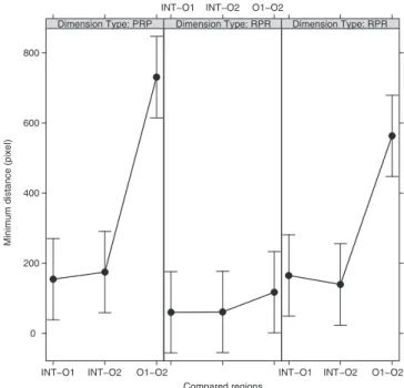
We calculated gap size as the Cartesian minimum distance between two polygons using the R package‘rgeos’ (Bivand & Rundel, 2015). The average minimum distance between a pole and the intermediate region was smaller than 200 pixels, corresponding to approximately 12% and 19% of the screen width and height respectively. The average distance between the poles was on average 30% of the screen width and 45% of the screen height. The statistical analysis, showed a main effect of Re-gions (χ2(2, N = 19) = 694.339, p < 0.0001) with the distance be-tween the two opposite poles bigger than the distance bebe-tween either of the two poles and the intermediate region (post hoc: O1–O2 vs. INT–O1: EST = 343.925, SE = 15.102, t-ratio = 22.773, p < 0.0001; O1–O2 vs INTeO2: EST = 345.398, SE = 15.102, t-ratio = 22.871, p < 0.0001). The interaction between the regions and Dimension Types was also significant (χ2(4, N = 19) = 267.278, p < 0.0001; effect size of Images: 12% of the total variance of the response variable Distance between the areas). The distance between O1 and O2 was smaller when the intermediate region was a point, i.e., for Dimension Type RPR, and larger when the intermediate region was a range, i.e., for Dimension Type PRP (EST = 613.537, SE = 78.576, t-ratio = 7.808, p < 0.001) and RRR (EST = 445.943, SE = 78.576, t-ratio =−5.675, p < 0.001). No difference in the distance between O1 and O2 was found between the two Dimension Types with a range INT, i.e., PRP and RRR (EST = 167.594, SE = 78.576, t-ratio = 2.133, p = 1).

Conversely, the size of the gaps left by participants between inter-mediate regions and poles did not differ significantly across any of the Dimension Types. None of the post hoc tests comparing the distances INT–O1 and INT–O2 across the Dimension Types was significant. 3.2.3. Eye movements

Fixations were detected with BeGaze (v. 3.5) using default settings for the“Low speed detection”, i.e., using an 80 ms minimum duration and a 100 pixel maximum dispersion.

Target Proportional extension 0.1 0.2 0.3 0.4 0.5 Dimension Type: PRP O1 INT O2 O1 INT O2 O1 INT O2

Dimension Type: RPR Dimension Type: RRR

Fig. 4. Average proportional extension of the outlines drawn by the participants. Data are divided by Dimension Type. Error bars represent 95% conﬁdence intervals.

Compared regions

Minimum distance (pixel)

0 200 400 600 800

INT−O1 INT−O2 O1−O2

Dimension Type: RPR

INT−O1 INT−O2 O1−O2

Dimension Type: RPR Dimension Type: PRP

Fig. 5. Average minimum distance between two areas outlined by participants. Error bars represent 95% conﬁdence intervals.

(9)

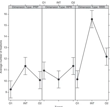
3.2.3.1. Number of fixations. We analysed the effects of Target and Dimension Type on the number offixations made by the participants before they made their decisions (a summary of the data is reported in Table 2) using a GLMM (Poisson family). The interaction between Dimension Type and Target was significant (χ2(4, N = 25) = 113.089, p < 0.0001; effect size of Images: 11% of the total variance of the Number offixations response variable). Post hoc tests revealed three aspects of this interaction (see alsoFig. 6).

The average number offixations associated with the identification of a point region did not differ significantly when that region was O1, O2 or INT– none of the post hoc tests between point INTs and point poles was significant. In other words, when the Target is a point, there is no difference between INTs and poles. The identification task (in terms of number offixation) was equally easy or difficult in all cases. This was true also for the identification of range regions. Post hoc tests revealed that the identification of range poles (O1 or O2) in Dimension Types RPR and RRR required a similar number of fixations as the identification of range INT in Dimension Type PRP. Only in Dimension Type RRR, where poles and INTs are all range regions, did the parti-cipants make morefixations when they were looking for INT than for O1 (EST = 0.421, SE = 0.033, z-ratio = 12.658, p < 0.0001) and O2 (EST = 0.237, SE = 0.031, z-ratio = 7.493, p < 0.0001). It should be noted that the number offixations made when the participants were looking for range INT in RRR Dimension Type was not significantly different from the number of fixations made when they were looking for range poles in RPR or range INT in PRP Dimension Types.

Secondly, in general, the identification of range regions did not require morefixations than the identification of point regions. In fact, when looking for range poles, the participants did not make more fixations than when they were looking for a point region, irrespective of Target (O1, O2 or INT). Only when the Target was an INT region in the RRR Dimension Type, did the participants make more fixations than when they were looking for point O1 (EST = 0.529, SE = 0.123, ratio = 4.291, p < 0.0001), point O2 (EST = 0.438, SE = 0.123, z-ratio = 3.561, p < 0.013) or point INT (EST =−0.429,SE = 0.123, z-ratio =−3.488, p < 0.02).

3.2.3.2. Fixation location. A preliminary inspection of the distribution ofﬁxations in the images was provided by the heatmaps, some of which are shown inFig. 7. The heatmaps suggest that when the task was to

identify the INT in the RPR Images, i.e., in the two central rows in Fig. 7, thefixations were mainly located in one area, but they were scattered across a larger area when the task was to identify either O1 or O2. The opposite pattern was observed in the PRP Images, see the two bottom rows of theFig. 7. When the task was to identify O1 or O2, the fixations clustered in a relatively limited area of the image, while when the task was to focus on the INT area, thefixations were scattered across a larger area.

In the case of the RRR Images (the top rows ofFig. 7), the pattern was less symmetrical. ForDENSEandNEAR, theﬁxations are concentrated

within one of the poles rather than the opposite poles, also when the task was to identify the INT region. It is possible that the participants used these two poles as anchors to identify the other two regions in the Images.

In order to interpret these patterns in a meaningful way, we made use of the participants own outlines of the Target regions. For every participantfixation,3_{we determined the distance to the three outlines} drawn for O1, O2 and INT, and which of the three regions was closest to thefixation. This allowed us to be able to specify how many fixations were closer to the Target region (“on-target fixations”) and how many were closer to one of the other two regions (“extra-target fixations”). In the latter case, we could also estimate if one region was more frequently looked at than the other, and if so, which one. The distances were calculated using the R-package‘rgeos’. Instances of fixations equidistant from two regions were excluded (2.6% of the data).

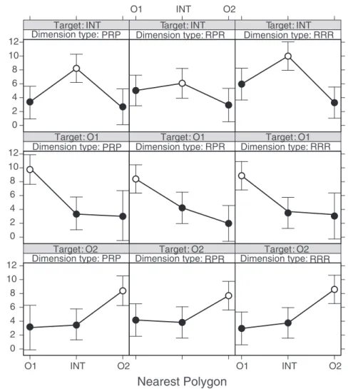
Wefirst focused on the fixations when the task was to look at the INT region, and conducted a GLMM (Poisson family, with Dimension Type and Nearest Polygon asfixed factors) on the subset of the Target INT only. Both factors (Nearest Polygon: χ2(2, N = 19) = 434.226, p < 0.0001; Dimension Type:χ2(2, N = 19) = 7.382, p < 0.05) and their interaction (Nearest Polygon∗ Dimension Type: χ2(4, N = 19) = 39.759, p < 0.0001) were significant. Post-hoc tests allowed us to interpret these results from the point of view of two main questions: (i) Where did the participants look most often when they were looking for the INT region? And (ii) where did they look most often when the fixations were not on the INT region?

The answers to these questions are given in the graphs on thefirst row inFig. 8. On-targetfixations were more frequent than extra-target fixations. The difference within the PRP Dimension Type was sig-nificant between INT and O1 (EST = 0.883, SE = 0.083, z-ratio = 10.590, p < 0.0001) and INT and O2 (EST = 1.072, SE = 0.108, z-ratio = 9.881, p < 0.0001). Within the RRR Dimension Type, the difference between INT and O1 was also significant (EST = 0.545, SE = 0.064, z-ratio = 8.427, p < 0.0001) and also be-tween INT and O2 (EST = 1.062, SE = 0.072, z-ratio = 14.571, p < 0.0001). Within the RPR Dimension Type, the difference between INT and O2 was significant (EST = 0.759, SE = 0.100, z-ratio = 7.571, p < 0.0001), but not between INT and O1 (EST = 0.184, SE = 0.077, z-ratio = 2.391, p = 0.604).

Furthermore, within the PRP Dimension Type, participants did not look signiﬁcantly more often at either O1 or O2 (EST = 0.188, SE = 0.127, z-ratio = 1.485, p = 1). However, within the RPR Dimension Type, participants did look more often at O1 than O2 (EST = 0.575, SE = 0.104, z-ratio = 5.486, p < 0.0001). In other words, when looking forNEITHER IN FRONT OF NOR BEHIND, the participants

madeﬁxations onIN FRONT OFmore frequently than onBEHIND, and when

looking forNEITHER ABOVE NOR BELOW, theyfixatedABOVEmore frequently thanBELOW. A significant difference between O1 and O2 was also found

within the RRR Dimension Type (EST = 0.517, SE = 0.085, z-ratio = 6.046, p < 0.0001). When looking for NEITHER NEAR NOR FAR AWAY, they made moreﬁxations onNEARthan onFAR AWAY, and when Target

Average number of fixations

9 10 11 12 13 14 15 16 O1 INT O2 Dimension Type: PRP O1 INT O2 Dimension Type: RPR O1 INT O2 Dimension Type: RRR

Fig. 6. Average number offixations in the identification of the poles and the intermediate regions for the three Dimension Types. Error bars represent 95% confidence intervals.

3_{We decided to focus on all}_{fixations rather than on only the first fixation since the} latter largely depends on early low-level properties of the image and often manifests a central bias (seeTatler, 2007).

(10)

looking forNEITHER DENSE NOR SPARSE, they made moreﬁxations onDENSE

than on SPARSE. This is evidence of an asymmetrical relationship

be-tween the two poles in the identiﬁcation of the intermediate region. For

NEAR andFAR AWAY, the result might be natural since the instructions

speciﬁed anchor points (near/far away from the dot/the sea/the stage), but this was not the case forDENSEandSPARSE. We can exclude that this was simply due to a generic spatial bias since the part of the Image showing DENSEwas in the top-right-hand side area of one Image (the

lines), in the bottom part of the second Image (ﬁsh) in the center-left-hand side area of the third Image (square dots). Similar patterns hold forABOVEandBELOW, andIN FRONT OFandBEHIND. ABOVEwas always

re-presented in the top half of the screen, whereasIN FRONT OFappeared in

different parts of the Images. It was situated in the top left-hand side area in one Image (cars in a lane), in the top right-hand side area of the second Image (climber), and in the center-right-hand side area in the third Image (point in a band arrow). Since O1 was the less extended pole along each dimension, it is still an open question whether this asymmetry between the two poles is due to the specific content of the properties constituting pole O1 of each dimension, or whether it is due to the characteristic of being O1 the less extended pole (we return to this issue in thefinal discussion).

Two additional GLMMs were conducted in order to study the ﬁxa-tions made by participants when looking for the poles. One GLMM was conducted on the subset of the data of the Target O1 (see the graphs in

the second row ofFig. 8) and another on the subset of the Target O2 (see the graphs in the third row ofFig. 8). In both analyses, the inter-action between Dimension Type and Nearest Polygon was signiﬁcant (GLMM on O1: χ2(4, N = 19)= 146.947, p < 0.0001; GLMM on O2:

χ2(4, N = 19)= 208.49, p < 0.0001). Also in this case, we present the

results with the two questions in mind: (i) Where did the participants look most often when they were looking for O1 or O2, and (ii) where did they look most often when theﬁxations were not on the target?

The answer to thefirst question is straightforward and consistent across the three Dimension Types (seeTable 3, the top two panels). On-targetfixations were more frequent than extra-target fixations; that is, when participants were looking for one pole, their fixations were mostly directed toward the region that they then outlined as showing that pole, and less frequently toward the INT region (see Table 3, Contrasts O1–INT and O2–INT) and the opposite pole (see Table 3, Contrasts O1–O2 and O2–O1).

The answer to the second question is that, overall, there were as many extra-targetfixations on the INTs as on the opposite pole, but more extra-target fixations on INT than on O2 within the RPR Dimension Type. This is shown inTable 3, in the bottom panels, where none of the constrasts INT–O1 (when the target was O2) and only one contrast INT–O2 (when the Target was O1) were significant. These results suggest that, for the identification of one of the poles, the INT region was as relevant as (and in one case even more relevant than) the

Fig. 7. Examples of heatmaps representing where the par-ticipants looked when asked to identify one of the three target areas. Each image shows the gaze behavior across all participants.

(11)

identiﬁcation of the opposite pole.

On the other hand, the comparison between the number of extra-targetfixations made on O1 when O2 was the Target, and vice versa (on O2 when O1 was the Target) raises the question whether the identifi-cation of one of the poles was more dependent on the identification of the other pole. For the identification of the poles, it was not the case that there were significantly more fixations on O2 when O1 was the Target than on O1 when O2 was the Target, for Dimension Type PRP

(EST = 0.011, SE = 0.215, z-ratio = 0.051, p = 1), but there were signiﬁcantly more ﬁxations on O1 (ABOVEandIN FRONT OF) when O2 was

the Target than on O2 (BELOWandBEHIND) when O1 was the Target, along

the RPR Dimension Type (EST = 0.589, SE = 0.131, z-ratio = 4.497, p = 0.002). Both these results are in agreement with the relative weight of the two poles (O1, O2) found when the Target was INT. Conversely, we did notfind signficantly more fixations on O1 (NEARandDENSE) when O2 was the Target than on O2 (FAR AWAYandSPARSE) when O1 was the

Nearest Polygon

Average number of fixations

0

2

4

6

8

10

12 O1

INT

O2

O1

INT

O2

0

2

4

6

8

10

12

0

2

4

6

8

10

12 Dimension type: PRP

:

Target INT

O1

INT

O2

:

Target INT

:

RPR

RRR

:

Target O1

:

Target O1

:

PRP

RPR

RRR

:

Target O2

:

Target O2

:

PRP

RPR

RRR

Dimension type:

Fig. 8. Average number offixations around the poles (O1, O2) and the intermediate region (INT), when the partici-pants were looking for the three Targets: INT (graphs on thefirst row), O1 (graphs on the second row), and O2 (graphs on the third row). The data are divided by Dimension Type (first column: PRP; second column: RPR; third column: RRR). White dots indicate on-target fixa-tions, and black dots indicate extra-targetfixations.

Table 3

Bonferroni post hoc comparisons referred to the diagrams in the second and third row ofFig. 8. Thefirst two panels at the top refer to the contrasts between on-target fixations and extra-targetfixations, the third panel refers to the contrast between extra-target fixations.

Target Contrasts Dimension Type Post hoc tests

O1 O1–INT PRP EST = 1.123, SE = 0.092, z-ratio = 12.265, p < 0.0001

RPR EST = 0.738, SE = 0.077, z-ratio = 9.480, p < 0.0001

RRR EST = 0.986, SE = 0.082, z-ratio = 12.008, p < 0.0001

O1–O2 PRP EST = 1.498, SE = 0.152, z-ratio =−9.802, p < 0.0001

O2 O2–INT PRP EST = 0.860, SE = 0.076, z-ratio = 11.207, p < 0.0001

O2–O1 PRP EST = 0.882, SE = 0.159, z-ratio = 5.538, p < 0.0001

O1 INT–O2 PRP EST = 0.374, SE = 0.168, z-ratio =−2.223, p = 0.942

RRR EST = 0.072, SE = 0.166, z-ratio = 0.438, p = 1

O2 INT–O1 PRP EST = 0.022, SE = 0.168, z-ratio = 0.133, p = 1

RPR EST =−0.142, SE = 0.100, z-ratio = −1.415, p = 1

(12)

Target for Dimension Type RRR (EST =−0.012, SE = 0.166, z-ratio =−0.073, p = 1), which is diﬀerent from what we found for the same Dimension Type when INT was the Target. In other words, for the Dimension Type RRR, it was only when the participants were looking for INT that one of the poles attracted moreﬁxations than the opposite pole.

3.2.3.3. Fixation duration. Fixation duration is often associated with, and modulated by, ongoing perceptual and cognitive processes (Henderson, 2007). InSection 3.2.1, we already discussed how long participants explored the Image before they started to draw the outline of the Target area, i.e., the overall identification time. However, this same identification time can be caused either by few, but long fixations, or many but shortfixations. For this reason, we also analysed fixation duration depending on the Dimension Type, the Target area, and the location of thefixations in terms of the nearest polygon.

A LMM (Gaussian Family) was run on the averagefixation duration (with Target, Dimension Type, and Location asfixed effects). The main effect of Target was significant (χ2(2, N = 19) = 24.677, p < 0.0001; effect size of Images: 10% of the total variance of the Fixation location response variable). Fixations made when the participants were looking for INT were on average longer than those made when they were looking for O1 (EST = 74.965, SE = 18.91, t-ratio = 3.964, p < 0.001) but not O2 (EST = 30.520, SE = 17.461, t-ratio = 1.748, p = 0.242). The two significant interactions (Target ∗ Nearest Polygon: χ2(4, N = 19) = 54.541, p < 0.0001; Dimension Type ∗ Nearest Polygon:χ2(4, N = 19) = 21.522, p < 0.001) showed that fixations on INT were longer than those on O1 or O2 only when INT was the Target and when INT was a point, i.e., for the RPR Dimension Type (INT–O1: EST = 140.097, SE = 27.867, t-ratio = 5.027, p < 0.0001; INT–O2: EST = 178.458, SE = 29.961, t-ratio = 5.956, p < 0.0001).

4. General discussion

With an increase of interest in and an awareness of the importance of perceptual grounding for language and cognition (e.g., Barsalou, 1999, 2010; Bergen, 2012; Caballero & Paradis, 2015; Gärdenfors, 2014; Paradis, 2015a, 2015b; Pecher & Zwaan, 2005; Zwaan & Taylor, 2006), a lease of new life has been given to research on dimensions and opposition (Bianchi et al., 2011; Bianchi et al., 2013; Bianchi et al., 2014; Bianchi & Savardi, 2008; Bianchi, Savardi, & Burro, 2011; Bianchi, Savardi, Burro, & Torquati, 2011; Jones et al., 2012; Kelso & Engstrøm, 2006; Paradis et al., 2015; Savardi, 2009; van de Weijer et al., 2012, 2014). What these approaches have in common is a general interest in the grounding of opposition (perceptual, physiolo-gical, or neuropsychological). The focus in all these studies has been on dimensionality and on opposites, but only in two of them (Bianchi et al., 2011; Bianchi et al., 2013), the nature of intermediate regions has been addressed.

In the present paper, we report on an investigation of six spatial Dimensions and their various intermediate and polar structures using a combination of eye-tracking and drawing methodologies. We focused on the extensions and placements of the three regions, on differences with respect to whether the regions were points or ranges and, in ad-dition to those parameters, we also examined how the participants went about identifying them. The outcome of the experiments was clear; the six spatial dimensions studied belong to three different Dimension Types: PRP, RPR and RRR. Each Dimension Type was represented by two Dimensions and each Dimension was instantiated in three different scenarios in the stimulus Images. In contrast to the extensive literature in psychology, cognitive science and linguistics on spatial expressions, scenarios and reference frames, and how they differ cross- culturally, (e.g., Carlson-Radvansky & Irwin, 1993; Carlsson-Radvansky & Logan

Gordon, 1997; Coventry & Garrod, 2004; Coventry,

Griﬃths, & Hamilton, 2014; Coventry, Prat-Sala, & Richards, 2001; Levinson, 2006; Li, Carlson, Mou, Williams, & Miller, 2011; Paradis

et al., 2013), we used the diﬀerent scenarios as representatives of the various

experiential contexts, and the six specific spatial dimensions as re-presentatives of the three Dimension Types. Our purpose was not to determine the impact of these various scenarios or different perspec-tives and ways of viewing spaces (e.g., Carlson-Radvansky & Irwin, 1993; Carlsson-Radvansky & Logan Gordon, 1997; Coventry & Garrod, 2004; Coventry et al., 2014; Coventry et al., 2001; Li et al., 2011; please note that the effect size of Images, in all our analyses, ranged in be-tween 8% and 16% of the total variance of the response variables considered). Like inBianchi et al. (2011)andBianchi et al. (2013), the underlying idea was that the application of a certain dimension in the different contexts may modify the relative extension of the three re-gions O1, INT, O2 (as indeed was the case, if we compare the relative size of O1 and O2 in our study with the proportional extensions re-ported inBianchi et al., 2011). The structure of the dimensions, how-ever, was expected to be invariant across the Dimension Types, i.e., the RRR, RPR or PRP structures. The average proportional extensions of O1s, O2s and INTs found in this study (Fig. 4) were congruent with the topological classifications reported in previous work (seeBianchi et al., 2011; Bianchi et al., 2013), where completely different tasks and visual stimuli were used. In what follows, we discuss and assess the main results of the study in accordance with the predictions stated inSection 3, and in relation to relevant previous work on this topic.

Firstly, the results partially confirmed prediction 1. We did not find evidence that intermediates in general took longer to identify than the opposite poles. The identification time for INT was longer than for O1, but the same as for O2 (Section 3.2.1). This finding is in line with previous work, showing that rating the experience of INTs in pictures of various ecological scenes was not more time-consuming than rating the experience of O1 and O2 (Bianchi et al., 2013), and hence the identi-fication of intermediates does not seem to be based on a mental process of double exclusion of the poles as suggested by the expression neither one nor the opposite pole. However, in this context it deserves to be pointed out that as part of the design of this study, O1 and O2 were ordered post hoc, based on the proportional extension of the two poles (with O1 as the less extended pole). This classification principle might be the reason for the faster identification times of the O1 pole, which is smaller as compared to the more extended O2 pole.

Secondly, we explored the number offixations needed for the iden-tification of the intermediates and the poles, and found that in general the identification of range INT did not require more fixations than the identification of range O1 and O2; the only exception was that range INT required morefixations than range poles in the RRR Dimension Type (seeSection 3.2.3.1). The identification of point INT did not re-quire morefixations than the identification of point O1 or O2. Again, thesefindings support the conclusion that, in general, the process of identifying intermediates and poles is similar. Intermediates do not seem to have special status as compared to the poles in terms of number offixations.

Furthermore, we analysed the location of thefixations (seeSection 3.2.3.2). Also from these data, a similar pattern of recognition of poles and intermediates emerged since in both cases the participants made morefixations on the Target Region than on either of the other two regions. The intermediate region supported the identification of one of the poles as much as the opposite pole did. When asked to identify the poles, the participants looked at the intermediates at least as often as they looked at the opposite pole. This result confirmed prediction 2 that the identification of the poles is dependent on the identification of the intermediates to the same extent as the other way around. Also, the analysis of thefixation locations suggested that the poles either had a symmetrical or an asymmetrical role in the identification of the three regions depending on the Dimension Type. O1 and O2 were looked at roughly to the same extent for the PRP Dimension Type, when INT was the Target, but there were morefixations on O1 than on O2 in the other two Dimension Types. Moreover, when one of the poles was the Target

(13)

and when the Dimension Type was RPR, the participants made more extra-target fixations on O1 when looking for O2 than extra-target fixations on O2 when looking for O1. The general picture suggests a prominent role of one of the two opposites. In light of the fact that three different Images were presented for each Dimension Type, there are reasons to believe that this asymmetry might reflect a genuine asym-metry of the two poles, rather than characteristics related to the par-ticular stimuli used in this study. However, since O1 by definition was the smaller pole, this asymmetry may also indicate that, for dimensions comprising Range poles, it is the less extended pole that is more in-formative and therefore looked at more. Further investigations are needed to determine this. An interesting angle would be to extend the investigation not only to dimensions with a topologically symmetrical structure, i.e., where both poles are points or ranges, but also to di-mensions with a point pole and a range pole, e.g., CLOSED–OPEN, REG-ULAR–IRREGULAR.

Some differences between intermediates and poles emerged with regard to the average duration offixations. On-target fixations on INTs, and in particular fixations on point INTs, were longer than fixations made on the poles (Section 3.2.3.3).

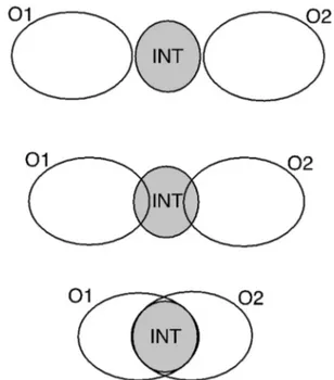
Thirdly, we examined whether and to what extent there were gaps or overlaps between the three regions drawn by the participants (Section 3.2.2.2). It was shown that overlaps between adjacent regions were negligible. More often than not, the regions were separated by a gap (INT–O1 and INT–O2 inFig. 5). Small gaps or small overlaps between INT–O1 and INT–O2 (as can be seen in the middle diagram inFig. 9, and as also found inBianchi et al., 2013) may be an indication that the participants were uncertain about the boundaries between adjacent regions. The combination of the fact that there was virtually no overlap between the regions and that the size of the gaps was small suggests that each of the Target areas could be identiﬁed relatively easily and straightforwardly by the participants. This was true irrespective of whether the adjacent regions were a point and a range, or two ranges. The general absence of overlap suggests that the participants mapped each Target property (O1, INT and O2) onto diﬀerent parts of the Images, as illustrated in the top diagram ofFig. 9. They rarely attrib-uted the same part to more than one of the three regions.

Theﬁnding that O1 and O2 did not overlap supports, in terms of perceptual evidence, the idea that the opposite poles are mutually ex-clusive. Theﬁnding that intermediates did not completely coincide with

the poles, as shown in the diagram at the bottom ofFig. 9, supports the idea that INT is not the same as O1 and O2, but has an identity of its own. This may sound counterintuitive if one thinks that in real life intermediates are often created by mixing opposites, for instance, by putting some drops of black color into white color to create gray color, or by adding some cold water to make hot water lukewarm. Indeed, it is not the case that our direct experience of gray is something that is black and white, or that our experience of lukewarm is something that is cold and hot. Confusing what we know about the process of producing something with how we perceive something is what in psychology of perception is called‘the stimulus error’. The results presented in this study are compelling evidence of the equal-status claim and the in-dependence of intermediates.

Fourthly, the results in this study are consistent with the original work byBianchi et al. (2011)on the spatial extensions of ranges and points. Our results (Section 3.2.2.1) strengthen the characterization of the perceptual structure of the Dimension (PRP, RPR and RRR). Irre-spective of whether they are poles or intermediates, points corre-sponded to proportionally smaller regions than ranges.

Importantly, the three types of configurational structure (R and P) analysed in this paper in relation to different Dimension Types (PRP, RPR, RRR), and the different Image Types do not necessarily apply to different objects or property dimensions, but may also apply to the same dimension. The three types identify different ways in which hu-mans organize their perceptual experience of the world. Along the

COLD–HOTscale of temperature, we may refer to human perceptual

ex-perience of some temperatures as hot at a given range of the scale, another as cold at a diﬀerent range of the scale and neither hot nor cold to yet another one. This is a RRR structure. But, when we use a ther-mometer to measure body temperature, 36.8° is the ideal temperature, and degrees below or above are too cold or too hot. In this case, we deal with the same physical scale (TEMPERATURE), but use a diﬀerent cognitive

structure, which is anchored in a well-deﬁned point of body tempera-ture; the poles are ranges on opposite sides of the point, along this RPR structure. In addition, yet another type of structure is compatible with the physical scale of temperature, namely the cognitive structure of

BOILING–FREEZING. Water boils at a precise temperature and freezes at another precise temperature; between those points there is a wide range of temperatures that are neither boiling nor freezing. This is a PRP structure.

An interesting continuation of the present study and previous stu-dies on the perceptual and neurocognitive grounding of opposites is to determine whether the results of the perception of opposites and in-termediates in spatial (visual) dimensions can be generalized to other perceptual dimensions. Do these results also hold for dimensions re-lated to sound, smell, taste, touch, force and movement? This is an intriguing question since descriptions of phenomena in all the mod-alities, including vision, make use of the same dimensional properties, albeit instantiated in diﬀerent meaning domains (Paradis, 2015b). For instance, long road, long taste, deep color, deep smell, sharp sounds, sharp smells, sharp tastes, sharp edges, sharp colors. This suggests that there is something more general across these structures and their instantiations in diﬀerent domains (Picard, Dacremont, Valentin, & Giboreau, 2003; Gärdenfors, 2014; Martino & Marks, 2001; for claims that pre-verbal perception is synaesthetic, see for instanceWalker et al., 2010).

We encourage attempts at a new take on how words actually mean in language and how we conceptualize the world in order tofind out to what extent perception is reflected in language and cognition. For re-searchers to succeed in this, we need to breathe fresh life into the basis of much research about the sensory-cognitive-language triad, in parti-cular into the modeling of language since it makes the basis for a large amount of research, not only in linguistics, but also in medicine, cog-nitive science, philosophy and psychology. We must dare to challenge established basic assumptions and move on to investigate fundamental issues on a large scale: Why is it that perceptual experience is talked about the way it is? Why is it that there are few domain specific words

Fig. 9. Diagrams representing three possible conﬁgurations of poles and intermediates based on diﬀerent amounts of overlap.