Dipartimento di Elettronica Informatica e Sistemistica Corso di dottorato in
Ricerca Operativa MAT/09 XXII CICLO
Coordinatore Prof. Lucio Grandinetti
Tesi di Dottorato
OMEGA
OUR MULTI ETHNIC GENETIC ALGORITHM
Carmine Cerrone
Il Relatore:
Prof. Manlio Gaudioso
Table of Contents i
Abstract iii
Introduction 1
1 Our Multi Ethnic Genetic Algorithm (OMEGA) 4
1.1 Introduction . . . 4
1.2 Our Multi Ethnic Genetic Algorithm (OMEGA) . . . 7
1.2.1 OMEGA Approach . . . 8
1.2.2 OMEGA’s steps . . . 10
1.2.3 Evolutionary Step Features . . . 12
1.3 Building Block and chromosome’s definition . . . 13
1.3.1 GA and OMEGA chromosome observation . . . 14
1.3.2 Basic ideas about the chromosome . . . 17
1.3.3 OMEGA and Blocks . . . 20
1.4 Minimum Labeling Spanning Tree . . . 21
1.4.1 Problem Definition . . . 22
1.4.2 The Algorithm . . . 22
1.4.3 Pseudocode . . . 28
1.4.4 Computational Results . . . 28
2 Monocromatic Set Partitioning 31 2.1 Problem Definition and Basic Notation . . . 31
2.2 Problem Complexity . . . 32 2.3 Mathematical Formulations . . . 35 2.4 Polynomial case . . . 40 2.4.1 Solution’s Optimality . . . 44 2.5 Genetic Approach . . . 47 2.5.1 The Chromosome . . . 48 i
2.5.2 The Crossover . . . 50
2.5.3 The Mutation . . . 50
2.5.4 The Splitting Population Function . . . 51
2.5.5 The Fitness Functions . . . 51
2.5.6 Pseudocode . . . 52
2.6 Results . . . 52
3 Bounded Degree Spanning Tree 55 3.1 Introduction . . . 55
3.2 Problem definition and motivations . . . 57
3.3 Mathematical Formulation . . . 59
3.4 Relations among MBV, MDS and ML . . . 64
3.4.1 Notations . . . 64
3.4.2 The problems are not equivalent . . . 64
3.4.3 Relations among the problems . . . 69
3.5 OMEGA Algorithm . . . 72
3.6 Results . . . 75
4 Multi-Period Street Scheduling and Sweeping (MPS3) 76 4.1 Introduction . . . 76 4.1.1 Variant 1 . . . 77 4.1.2 Variant 2 . . . 81 4.2 Literature Review . . . 82 4.3 Problem Formulation . . . 83 4.3.1 Variant 1 . . . 83 4.3.2 Variant 2 . . . 87 4.4 Genetic Algorithm . . . 87 4.4.1 Initialization . . . 88 4.4.2 Schedules . . . 89 4.4.3 Fitness . . . 93 4.4.4 Breeding . . . 93 4.4.5 Mutation . . . 97
4.4.6 Genetic Algorithm Summary . . . 98
4.5 Results . . . 100
Combinatorial optimization is a branch of optimization. Its domain is optimization problems where the set of feasible solutions is discrete or can be reduced to a discrete one, the goal being that of finding the best possible solution. Two fundamental aims in optimization are finding algorithms characterized by both provably good run times and provably good or even optimal solution quality. When no method to find an optimal solution, under the given constraints (of time, space etc.) is available, heuristic approaches are typically used. A metaheuristic is a heuristic method for solving a very general class of computational problems by combining user-given black-box procedures, usually heuristics themselves, in the hope of obtaining a more efficient or more robust procedure. The genetic algorithms are one of the best metaheuristic approaches to deal with optimization problems. They are a population-based search technique that uses an ever changing neighborhood structure, population-based on population evolution and genetic operators, to take into account different points in the search space. The core of the thesis is to introduce a variant of the classic GA approach, which is referred to as OMEGA (Multi Ethnic Genetic Algorithm). The main feature of this new metaheuristic is the presence of different populations that evolve simultaneously, and exchange genetic material with each other. We focus our attention on four different optimization problems defined on graphs. Each one is
proved to be NP-HARD. We analyze each problem from different points of view, and for each one we define and implement both a genetic algorithm and our OMEGA.
In the 1950s and the 1960s several computer scientists independently studied evolu-tionary system starting from the idea that evolution could be used as an optimization tool for engineering problems. The idea in all these systems was to let a population of candidate solutions to a given problem, evolve using operators inspired by natural genetic variation and natural selection. The approach was firstly introduced in 1954 in the work by Nils Aall Barricelli, who was with the Institute for Advanced Study in Princeton, New Jersey. [27] [2]. This publication was not widely noticed. Neverthe-less, computer simulation based on biological evolution became more common in the early 1960s, and the methods were described in books by Fraser and Burnell [16, 17]. Genetic algorithms (GA) in particular became popular thanks to the work by John Holland in the early 1970s, and particularly his book Adaptation in Natural and Ar-tificial Systems (1975) [21] . His work originated from studies of cellular automata, conducted by Holland and his students at the University of Michigan. Holland in-troduced a formalized framework for predicting the quality of the next generation, known as Holland’s Schema Theorem. In the last few years there has been widespread interaction among researchers studying various evolutionary computation methods, and it is quite hard to retrace the boundaries between GAs, evolution strategy, evo-lution programming, and other evoevo-lutionary approaches have broken down to same
extent. Nowadays researchers use the term ”genetic algorithm” to describe something very far from Holland’s original concept. Among the most famous GA variants, the Lemarcking evolution and the Memetic algorithms [12] play a crucial role. Grefen-stette introduced the Lemarckian operator into Genetic algorithms [20]. This theory introduces the concept of experience into the GAs, and suggest the use of a clever crossover technique. Moscato and Norman introduced the term Memetic algorithm to describe genetic algorithms in which local search plays a significant role [25]. There are several variants to the basic GA model, and in most cases these variants are com-bined to obtain the best solution to the specific problem. Another possible solution is the rank-based selection. We cite this technique in particular because the implicit splitting of the population in sub-populations and the concept of migration are largely used and reinterpreted in this work.
Genetic Algorithms are the logical thread that unifies all the chapters of the dissertation.
It is organized as follows. In chapter one we introduce the basic ideas of our multi ethnic genetic approach (OMEGA) and state it formally. The main feature of this new metaheuristic is the presence of different populations that evolve simultaneously, and exchange genetic material with each other. The applications are reported in chapter two three and four. In each of them a particular problem of graph optimization is studied. All studied problems are defined on a graph, and in all the cases we try to solve a combinatorial optimization problem via a GA. We introduce in the second chapter a problem defined on labelled graph, in this case we introduce two mathematical formulations and after a brief study of their complexity in general and in particular cases, we introduce a GA, able to find a solution very near to the
optimal one. In the third chapter we study a bounded degree spanning-tree problem, we present a tree variant about the same problem, we introduce some results about the relation between the problems, and we provide a branch and bound algorithm able to find the optimal solution. In the last section we use a GA. In the last chapter we focus our attention on a arch-routing problem on multigraph, for this problem we introduce a mathematical formulation and a GA. In this work we apply a GAs to three combinatorial optimization problems defined on a graph.
Our Multi Ethnic Genetic
Algorithm (OMEGA)
1.1
Introduction
The genetic algorithm is one of the best approaches to solving optimization problems. These algorithms are a population-based search technique that use an ever-changing neighborhood structure, based on population evolution and genetic operators, to take into account different points in the search space. Many techniques have been devel-oped to escape from the local optimum when genetic algorithms fail to individuate the global optimum. In any case it appears clear that the intrinsic evolution scheme of genetic algorithms cannot be enforced to avoid the local optima without upsetting the ”natural” evolution of the initial population.
In this work, in order to reduce the probability of remaining trapped in a local mini-mum we keep the basic schema of GA. The main difference is that, starting from an initial population, we produce, one by one, k different populations and we define k different evolution environments in which we left thek populations to evolve indepen-dently, Although an appropriate merging scheme, is embedded to guarantee possible
interaction.
John Holland showed in the book Adaptation in Natural and Artificial Systems (1975) [21], how the evolutionary process applied to solving a wide variety of problems. Many authors have in fact drawn inspiration from nature to create a highly adaptive optimization technique. In this work we take into account other characteristics of the evolutionary process, in order to improve the performance and the flexibility of the classic genetic algorithm; our approach uses the concept of Speciation to increase the amount of the analyzed solutions.
To achieve this aim we modify three different components of a GA: • The population.
• The fitness functions.
• The chromosome representation.
In an evolutive process the aim of each individual is reproduction. Obviously in the world the resources are limited and for this reason, it isn’t possible that every one of the individuals will be able to reproduce. In this way only the strongest ones can achieve their goal of producing offspring for the next generation. These pro-cesses from generation to generation have produced bodies perfectly adapted to their environment. This brief description of the Darwinian principle of reproduction and survival of the fittest is the basis of the current GA.
An important observation is in order make. If the goal of each organism is the same, why do we have many different species? There are two basic reasons: (i) There are many streets which arrive at the same place; (ii) to survive you must adapt to the environment. Usually in a GA approach we observe the evolution of a population from a basic set of individuals to a set of relatives who are better adapted to the prob-lem. This strategy does not take into account the option of producing from the same species, different races. The idea at the basis of our approach is that, when ever many different races are involved in the same evolutionary process, the genetic difference between the populations can increase the quality of the results of all the process. In other words using this technique we can try to escape from a local minimum solution, creating new populations that evolve independently. The use of different variants of the same fitness function, is adopted to guarantee that different populations do not take the same evolutionary path.
The main idea of our technique consists of translating the concept of genetic iso-lation and genetic convergence from a biologic context into an algorithmic approach. This work introduces a modified GA approach that draws its inspiration from two fundamental biological concepts: Speciation and Convergent Evolution.
Speciation is the evolutionary process by which new biological species arise. There are four geographic modes of speciation in nature, based on the extent to which speciating populations are isolated from one another.
Convergent evolution describes the acquisition of the same biological trait in un-related populations. The wing is a classic example of convergent evolution in action. Although their last common ancestor did not have wings, birds and bats are fitted
with wings, similar in construction, due to the physical constraints imposed upon wing shape.
Our main item is to design a genetic schema able to escape from a local minimum solution. The concept of Convergent Evolution suggests to us that if we simply design a multi-start genetic algorithm, there is a great probability of obtaining similar results from any instances. On the other hand, the concept of Speciation tells us that if a population is branched into two or more sub populations forced to adapt to new environments, in a short period any population can probably evolve into a new species.
1.2
Our Multi Ethnic Genetic Algorithm (OMEGA)
A main issue regarding metaheuristic approaches in general and genetic algorithms in particular is how to avoid to be trapped in local minima while exploring the largest possible feasible region. This problem has particular relevance when the objective function is characterized by a large number of local minima. In the next example we show the function f1 = 5∗ sin(12x) + (101x)2 . If our objective is to find the minimum of f1, our genetic algorithm can be trapped in any of the many minimal solutions.
-50 0 50 50
In these cases, in order to avoid to remain trapped in local minima, various tech-niques can be applied:
• We can work on the crossover operators. Although all crossover operators are designed to take potentially large steps, many analytical results show that the crossover tends to make its largest jumps during the first few generations be-cause it takes advantage of the diversity in the population.
• We can work on the mutation operators. But usually, in order to ensure the convergence of this method, large steps are not desirable in this phase.
• We can use the multi-start technique, but the biological concept of convergent evolution suggests that there is a concrete probability of creating many similar populations. Moreover, a multi-start technique usually does not use information from the previous iteration in the next population.
In the rest of this chapter we will describe our genetic approach and how it is related to the above mentioned issues.
1.2.1
OMEGA Approach
OMEGA approach takes inspiration from the biological concept of genetic Isolation and Speciation; moreover it leans on the building-block hypothesis (Holland, 1975; Goldberg, 1989).
Using a classical genetic algorithm we create a population P0. After a sufficient number of iterations (i), we have a population Pi containing descendants of the best
solutions found. In this population the rate of good features (blocks) is high (building-block hypothesis) [15]. We consider this population a new biological species and we
try to get the process of Speciation by splitting the population. The new populations are immersed in different environments in order to minimize convergent evolution. This ensures the formation of different species, compatible with each other in terms of building-blocks. After a sufficient number of iterations, this process can be iterated, creating and merging a random number of populations.
Consider for instance the following problem:
minf1 (1.2.1)
x ∈ < (1.2.2)
where f1 is the previously defined objective function.
By using a classical genetic algorithm, we could get stuck in a local minimum with high probability.
Now let’s consider the above presented technique. We split the population P derived from the classical genetic algorithm in P1 and P2. These two populations will evolve indipendently, but for P2 we consider a different fitness functionf2 = 5+(101x)2 as shown in figure 1.2.
-50 0 50 50
Figure 1.2: f2
the two populations again, the new population P subject to function f1 can take advantage of the building-blocks that led P2 to the solution 0 to expand its genetic diversity and possibly improve the solution for the original problem.
1.2.2
OMEGA’s steps
In this section we present the basic scheme of our OMEGA approach. It is easy to understand that all the concepts introduced in this approach can to be combined in several ways. In the following we introduce a very easy pattern, useful to understand the approach. In the other chapters of this dissertation we apply this algorithm to different problems and in some cases we introduce different patterns to mix the population.
Let G(x, P, f) be an evolutionary scheme, where x is the input instance, P is a population of solutions and f is the fitness function. Let f0 be the main fitness function of our problem, and let F = {f1, f2, . . . , fn} be a set of n fitness functions
related with f0.
Input: problem instance x. Output: a feasible solution of the given problem. 1. t = 0.
2. Creation Operation: Create Pt, the starting population for the problem.
3. Repeat until a given stopping criterion is satisfied:
(a) Execute G(x, Pt, f0) to obtain the evolved population ˆPt.
(b) Split Operation: Split ˆPt inP(t,1), . . . , P(t,k) populations
- Randomly select a fitness function fr∈ F
- Execute G(x, P(t,j), fr) to obtain the evolved population ˆP(t,j)
(d) Merge Operation: Merge populations ˆP(t,1), ˆP(t,2), . . . ˆP(t,k) to obtainP(t+1). (e) t := t + 1
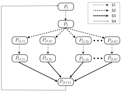
The basic version of the algorithm starts at timet = 0 from a unique population Pt
that evolves according to a given genetic schemeG and to the main fitness function f0. After this evolutionary step, the obtained evolved population ˆPtis split intok different
populations. Each obtained population evolves according to a given evolutionary scheme and a fitness function fr randomly selected among those in the set F . The
evolved populations are merged into a unique population Pt+1 and the process is
iterated until a given stopping criterion is reached (see figure 1.3). In the figure, lines S1,S2,S3,S4 represent respectively:
1. S1 : Evolutionary Step. 2. S2 : Split Operation. 3. S3 : Merge Operation.
4. S4 : Repeat until a given stopping criterion is satisfied.
The Split Operation takes as input a given population P and returns a set of k populations (P1. . . Pk). The k populations are obtained from P by partitioning it
into k sub-populations where k is a random value ranging from 2 to n. The size of each Pi is chosen either equal to
l|P |
k
m
or equal to j|P |k k such that Pk
i=1|Pi| = |P |.
The Merge Operation takes as input a given set of populations Pi and returns a
Figure 1.3: Block diagram of OMEGA’s Basic version
1.2.3
Evolutionary Step Features
When we speak about evolutionary steps, we refer to a sequence of j iterations of a classical genetic algorithm. In particular G(x, P, f) is a genetic algorithm, where x is the input instance, P is a population of solutions and f is the fitness function. The populationP is an input of the algorithm; after a fixed number of iterations, the genetic algorithm evolves P into a new population ˆP .
In this metaheuristic structure we can use any genetic algorithm. However, to fully exploit all the characteristics of the OMEGA it is important to pay particular atten-tion to two main aspects.
1. The chromosome’s definition :
of the solution after the crossover operation. In particular, in our metaheuristic we introduce the Merge operator. This operator simulates the migration of different ethnic groups (the populations P ) in the same environment. For this reason we want a chromosome able to preserve the features of the solution, although this solution is coupled to another of a different population.
2. The crossover’s definition :
The observations of the previous step imply the crossover’s importance. We can assert that the crossover and the chromosome definition are two of the most relevant items of a genetic algorithm and in particular these two aspects are fundamental for the creation of a multi ethnic genetic algorithm.
1.3
Building Block and chromosome’s definition
The Genetic algorithms are relatively simple to implement, but their behavior is dif-ficult to understand. In particular it isn’t easy understand why they often produce high quality solutions. One hypothesis is that a genetic algorithm performs adapta-tion by implicitly and efficiently implementing the building block hypothesis (BBH): a description of an abstract adaptive mechanism that performs adaptation by re-combining ”building blocks”. A description of this mechanism is given by (Goldberg 1989:41).
Anyway there are several results which contradict this hypothesis. The debate over the building block hypothesis demonstrates that the issue of how GAs ”work” is cur-rently far from settled. Nevertheless most solutions are designed taking into account the building block hypothesis.
1.3.1
GA and OMEGA chromosome observation
The main characteristic of OMEGA is the presence of different populations that evolve together. This characteristics does not imply any difference between this approach and a classic GA during the lifecycle of a population. On the other hand, when elements of different species are mixed in a unique population, we have to take into account this new situation. It is very important to create a strategy that ensures compatibility between individuals of different populations.
For example if our problem is to look for a Hamiltonian cycle in the graphG(V, E) (fig. 1.4) , we can use as a chromosome for the GA a {0, 1} vector associated with the edges.
Figure 1.4: G(V, E)
In fig. 1.5 we have a population of four elements. The elements are very different from each other. If we define a basic crossover function using the + operator we can produce six different new chromosomes. Figs. 1.6,1.7,1.8,1.9 show four of these solutions, where figs. 1.6,1.7 show two feasible solutions and figs. 1.8,1.9 show two
A B C D E F G H I L 1 1 1 0 0 0 0 0 0 0 chromosome 1 A B C D E F G H I L 0 0 0 1 1 1 0 0 0 0 chromosome 2 A B C D E F G H I L 1 0 0 1 0 0 0 1 0 0 chromosome 3 A B C D E F G H I L 0 0 0 0 1 0 1 0 0 1 chromosome 4
Figure 1.6: solution ch1 + ch2 Figure 1.7: solution ch3 + ch4
unfeasible solutions. It is easy to understand that if we have a population of such different elements it is very unlikely that we will produce feasible solutions.
For this reason if we have a GA that uses an unintelligent crossover it is necessary to balance two aspects: (i) we need a population composed of different elements to allow an evolution process and escape from the local minima; (ii) we need elements that are not very far from each other, in order to produce a stable and convergent search procedure.
These two aspects of a GA are very relevant when we define the structure of the chromosome. When we define the chromosome for the OMEGA this problem is accentuated. In a GA there is a single population and we can assume that the difference between two elements isn’t very big. The reason is that the two elements are evolved in the same population and are descendants of the same relatives. In an OMEGA we can merge different populations and it is possible to have a crossover between very different chromosomes.
To exploit this situation it is important to design a chromosome very accurately. In the following a basic idea to design a chromosome for the OMEGA is shown, as well as a possible application to the SpanningT ree problem.
1.3.2
Basic ideas about the chromosome
The aim of the OMEGA chromosome is to improve the crossover compatibility be-tween two individuals. A possible approach to achieve it is to define a structure that automatically focuses attention on some characteristics of the chromosome and tries to import it into the new generation. Using this approach the chromosome isn’t a rep-resentation of a solution but a data set that contains information about the creation
of new elements.
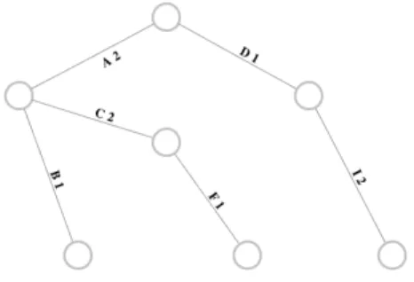
Figure 1.10: G(V, E)
It is easy to understand the idea by looking at an example. If our problem is to look for a particular (for example a bounded degree) spanning tree of a graphG(V, E) (e.g. the graph in fig. 1.10) , with|V | = k , we can use as chromosome C an integer vector with size greater than (k − 1). Each element of the vector represents an edge of G. We can have repetitions in C. Obviously C does not represent a spanning tree of G but it is possible to produce it using an easy procedure. We can associate a value to each edge that represents the number of occurrences that the edge has in C (fig. 1.11) .
Now, we can use an algorithm such as Kruskal or Prim to compute the minimum weight spanning tree of G. To obtain a feasible solution to our original problem.
Using this procedure the chromosome represents a suggestion for spanning tree procedure. Obviously by mixing different populations with elements very far from each other, we are sure that the ”suggestions” arriving from both the parents are taken into account in the child.
Figure 1.11: G(V, E) weighted graph
1.3.3
OMEGA and Blocks
In the previous section, we introduced a possible definition of the OMEGA chro-mosome. The structure is motivated by the necessity of improving the crossover compatibility between chromosomes.
The aim of this section is to add to the previous approach another idea. Essentially taking inspiration from the building block theory [21], we want to modify the chro-mosome’s structure, in order to preserve substructure information after the crossover. Our solution is to split the chromosome into sub-components, called blocks.
• Each block has a static or dynamic dimension, depending on the problem and the approach.
• The crossover isn’t able to modify a block, it can just recombine parents’ blocks. • The mutation is the only function able to modify a block, by adding or removing elements, changing elements, or deleting from or adding to a chromosome’s blocks.
In the figure 1.13 we can see three examples of OMEGA chromosomes. Each one of the three examples is related to the figure 1.10 of the previous page. The meaning for this chromosome is exactly the same one that we have used in the previous section. In this last step, we want to introduce a partition of the chromosome into sub-components.
Our intent is to create logical blocks able to describe little slices of a solution. In our opinion there are three consequences to using this approach.
• If a block describes part of a good solution, there is some chance that its in-troduction in another chromosome increases the fitness function, and for this
reason we can have more copies of the same block in the population.
• Iteration by iteration we can obtain an automatic partition of the instance into sub-problems, each one described by one or more blocks.
• The recombination of these blocks can increase the crossover’s compatibility between elements, in particular if the elements are very different from each other.
All the previous points are conjectures, but they represent an important part of the intuition that led us to design this technique. In the last section of this chapter, in order to better explain the OMEGA approach, we will apply the technique to a well known problem, the Minimum Labeling Spanning Tree (MLST).
A D A C B F I I C E chromosome A D I E F I A C B C chromosome 1 A C F C chromosome 2 D I I E A B A C chromosome 3 D I I E A B F C martedì 20 ottobre 2009
Figure 1.13: OMEGA’s chromosome examples
1.4
Minimum Labeling Spanning Tree
Given a connected, undirected graph whose edges are colored (or labeled), the mini-mum labeling spanning tree (MLST) problem seeks a spanning tree with the minimini-mum number of distinct colors (or labels). In this section we will use the OMEGA algo-rithm to solve the MLST problem. We chosen this problem because it is easy to understand and describe and because there are several papers that compare many
optimization techniques. Our goal is not to produce the best metaheuristic for the MLST but to compare our technique with other approaches.
1.4.1
Problem Definition
In the minimum labeling spanning tree (MLST) problem, we are given an undirected labeled graph G = (V, E, L), where V is the set of nodes, E is the set of edges, and L is the set of labels. We seek a spanning tree with the minimum number of distinct labels. This problem was introduced by Chang and Leu [9], who proved its NP-hardness by reducing it to a minimum cover problem. Since then, other researchers have studied and presented other heuristics for the MLST. Some references on this topic are [23, 7, 29, 11, 26, 6, 30]. In particular there are three works that introduce Genetic Algorithms for MLST [29, 26, 30].
1.4.2
The Algorithm
The structure of the algorithm is exactly the same as the one introduced in the section 1.2.2. To describe OMEGA as applied to the MLST it is sufficient to introduce the definition of the chromosome and explain how the crossover, the mutation and splitting population function work, and finally, to show the set of fitness functions.
The Chromosome
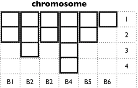
The first step to describe the chromosome is the introduction of two parameters W and H. They are used to describe the maximum dimensions of the chromosome. W represents the width of the chromosome, in particular the maximum number of blocks. H represents the height of the chromosome, corresponding to the maximum number
of elements for each block. We can introduce some limitations to the dimension of these parameters, W < |V | and H < |V |. However, in order to obtain an effective procedure, it is preferable to set the parameters according to the input instance. In the following experiments we used: W ← |V |10 and H ← 3.
chromosome 1 2 3 4 B1 B2 B2 B4 B5 B6 lunedì 26 ottobre 2009
Figure 1.14: OMEGA’s chromosome structure
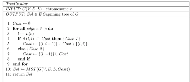
In figure 1.14 a chromosome composed of six blocks is presented. Each block has a dimension between one and four. Now we need a procedure that takes as input a chromosome and produces as output a spanning tree. In figure 2.6 such a procedure is presented.
The algorithm builds the set Cost, associating with each label a negative integer representing the occurrences of the label in the chromosome.
Using a Minimum Weight Spanning Tree procedure (MST) it is possible to build the solution. The MST takes into account as cost for each edgee :Sol(L(e)) .
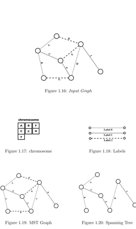
In the following we present an example that shows that it is possible to produce a spanning tree using the input chromosome. Using as input the graph of figure 1.16, G(V, E, L) , |V | = 7 ,
TreeCreator
INPUT: G(V, E, L) , chromosome c OUTPUT: Sol ∈ E Sapnning tree of G
1: Cost ← ∅
2: for all edge e ∈ c do 3: l ← L(e)
4: if ∃ (l, i) ∈ Cost then {Case 1 } 5: Cost ← {(l, i − 1)} ∪ Cost \ {(l, i)} 6: else{Case 2 } 7: Cost ← {(l, −1)} ∪ Cost 8: end if 9: end for 10: Sol ← MST (G(V, E, L, Cost)) 11: return Sol
Figure 1.15: Spanning Tree Generator L = {0, 1, 2} ,
and the chromosome
c = {{A, C, F }, {B, C}, {F, H}} of figure 1.17, the procedure TreeCreator builds
Sol = {(A, −1), (B, −1), (C, −2), (D, 0), (E, 0), (F, −2), (G, 0), (H, −1), (I, 0)} . In figure 1.19 the resulting graph is shown. Using a MST procedure, we are able to produce the spanning tree of figure 1.20, using just two different labels.
The Crossover
The crossover is the easiest function of OMEGA’s architecture. Basically the function takes as input two chromosomesc1, c2 and it produces as output the chromosome c3. The procedure randomly selects 50% of the blocks of c1 and c2, and it inserts the blocks into the new chromosome c3. In figure 1.21 a graphical example is shown.
Figure 1.16: Input Graph chromosome 1 2 3 4 B1 B2 B2 B4 B5 B6 A C F F H B C chromosome lunedì 26 ottobre 2009
Figure 1.17: chromosome Figure 1.18: Labels
chromosome 1 2 3 4 B1 B2 B2 B4 B5 B6 A C F F H B C chromosome A D I E F I A C B C chromosome 1 A C F C chromosome 2 D I I E A B Input: A D I E F I A C B C chromosome 1 A C F C chromosome 2 D I I E A B Selection: A D I E F I chromosome 1 chromosome 2 D I A B Selection: A D I E F I chromosome 3 D I A B Output: martedì 27 ottobre 2009 Figure 1.21: Crossover The Mutation
There are three different kind of mutation: MUT-ADD, MUT-DEL and MUT-CHANGE. The mutation operator randomly runs one of these three; if it isn’t possible to use MUT-ADD or MUT-DEL, MUT-CHANGE is used.
Respectively, the chances of selecting the operators are: 50%, 30%,20%.
• MUT-ADD randomly selects a block in the chromosome and if it isn’t full, it adds another edge in the last position. The new edge is selected from the set of edges near the connected structure, present in the same block.
• MUT-DEL randomly selects a block in the chromosome and if its dimension is greater than one, it removes a random edge from the block.
• MUT-CHANGE randomly selects a block in the chromosome, randomly selects an edge from the block, and replaces it with a new edge. The new edge is
selected from the set of edges near the connected structure, present in the same block.
The Splitting Population Function
The Splitting Population Function (SPF) is used to partition the original population into k sub-populations. This procedure is totally random, and if h is the dimension of the original population, it produces k new populations, each one of cardinality h
k. The aim of this procedure is to move the chromosomes of a big population into k different new populations.
The Fitness Functions
The fitness function is very easy to understand. It takes as input a chromosome c, using the procedure 2.6 to produce a spanning tree SP that is composed of |V | − 1 edges of the original graph G(V, E, L). It produces a set C including all the labels identified inSP , and the return value is equal to |C|. Now we want to identify other fitness functions related to the first one. This step is very easy. The procedure builds the function CT : L −→ R used to associate a numerical value to each label. The new fitness function is: f : P∀ l∈CCT (l). Obviously if for each label l ∈ L CT (l) = 1 we produce the original fitness function. When a new fitness function is randomly generated, it produces a function CT that produces one for most of the labels in L, but is able to produce a value greater than one for some labels.
Usually the procedure identifies some good solutions in the current population and tries to forbid the selection of one or more used labels.
1.4.3
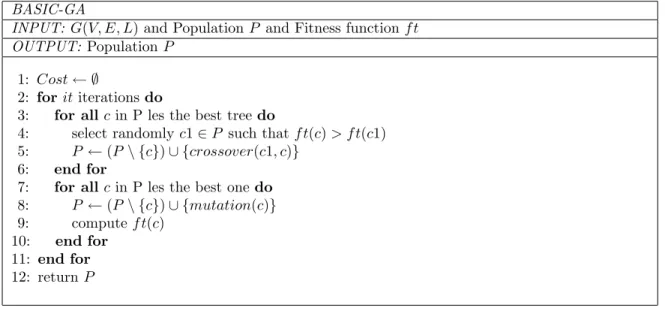
Pseudocode
BASIC-GA
INPUT: G(V, E, L) and Population P and Fitness function ft OUTPUT: Population P
1: Cost ← ∅
2: for it iterations do
3: for allc in P les the best tree do
4: select randomly c1 ∈ P such that ft(c) > ft(c1) 5: P ← (P \ {c}) ∪ {crossover(c1, c)}
6: end for
7: for allc in P les the best one do 8: P ← (P \ {c}) ∪ {mutation(c)} 9: compute ft(c)
10: end for 11: end for 12: return P
Figure 1.22: Basic Genetic Algorithm
1.4.4
Computational Results
This is a preliminary version of this section. We compared the OMEGA’s results with the results proposed in [7]. In fig.1.24 the first three columns show the parameters characterizing the different scenarios (n, l and d) n: number of nodes of the graph, l: total number of labels assigned to the graph, d: measure of density of the graph. The remaining columns give the results of the MVCA heuristic, Variable Neighborhood Search, Simulated Annealing, Reactive Tabu Search and the Pilot Method, respec-tively. All the values are average values over 10 different instances. The instances set is composed of 150 instances. In each row of the table in the figure we wrote in bold face the best results obtained by the different tested procedures. We can see that our approach OMEGA, except for one instance, is able to always find the best solution.
OMEGA
INPUT: G(V, E, L)
OUTPUT: Sol ∈ E Sapnning tree of G 1: P OP = {P0, P1, . . . P10} set of populations
2: |P0| = h
3: |P1| = |P2| = . . . = |P10| = 0
4: while Not End Conditions do 5: BASIC-GA(G, P0, f0)
6: if new best solution in P0 then 7: set new best solution
8: end if 9: SPF(P0) =⇒ |P0| ' |P1| ' . . . ' |P10| ' h 10 10: for allP ∈ P OP do 11: BASIC-GA(G, P, frandom) 12: end for 13: P0⇐ P1∪ P2∪ . . . P10 14: P1⇐ P2⇐ . . . ⇐ P10⇐ ∅ 15: end while Figure 1.23: OMEGA
n l d MVCA VNS SA RTS PILOT OMEGA 20 20 0,8 2,6 2,4 2,4 2,4 2,4 2,4 20 20 0,5 3,5 3,2 3,1 3,1 3,2 3,1 20 20 0,2 7,1 6,9 6,7 6,7 6,7 6,7 30 30 0,8 2,8 2,8 2,8 2,8 2,8 2,8 30 30 0,5 3,7 3,7 3,7 3,7 3,7 3,7 30 30 0,2 8,0 7,8 7,4 7,4 7,5 7,4 40 40 0,8 2,9 2,9 2,9 2,9 2,9 2,9 40 40 0,5 3,9 3,9 3,9 4,0 3,7 3,7 40 40 0,2 8,6 8,3 7,4 7,9 7,7 7,4 50 50 0,8 3,0 3,0 3,0 3,0 3,0 3,0 50 50 0,5 3,9 3,9 3,9 4,0 3,7 4,1 50 50 0,2 9,2 9,1 8,7 8,8 8,6 8,6 100 100 0,8 3,3 3,1 4,0 3,4 3,0 3,0 100 100 0,5 5,1 5,0 5,2 5,1 4,7 4,6 100 100 0,2 11,0 10,7 10,7 10,9 10,3 10,1 martedì 27 ottobre 2009
Monocromatic Set Partitioning
2.1
Problem Definition and Basic Notation
In this chapter we focalize our attention on a new problem, the ”monochromatic set partitioning” (MMP ) problem. Given a graph G with labels (colors) associated with the edges, a feasible solution for the MMP is a set of connected components of G such that each component is composed exclusively of monochromatic edges. We are looking for a feasible solution with the minimum number of monochromatic components. In the following we prove that MMP is NP-hard and we provide some mathematical formulations for this problem. Moreover we show a polynomial case and in the last part of this chapter we present an OMEGA approach to the problem. Let G = (V, E, C) be an undirected and edges labeled graph where V is the vertex set, E the edge set and C a set of labels. A label C (i, j) ∈ C is associated with each edge (i, j) ∈ E. A feasible solution for the MMP problem is a set of edges SOL ⊆ E such that for each two adjacent edges (i, j), (j, k) ∈ SOL, we have that C (i, j) = C (j, k) . The value of the objective function is equal to the number of connected components in the sub-graph of G induced by the edges set SOL.
Given a subsetS ⊆ E of edges, the set C (S) = S(i,j)∈SC (i, j) is the corresponding set of labels. The subgraph induced by a given label c ∈ C is denoted by Gc, i.e.
Gc = (V, Ec, c) with Ec = {(i, j) ∈ E : C (i, j) = c}. Similarly, we define Gc as the
subgraph of G without edges whose label is c, i.e Gc = (V, E \ Ec, C \ {c}). Let us
define Pc as the set of connected components in Gc, i.e. Pc = {Pc1, . . . , Pcr} where
Pj
c, 1 ≤ j ≤ r, is a monochromatic component whose color is c. The set of edges
incident to a vertex i ∈ V is denoted by δ(i) = {j : (i, j) ∈ E}. If |C (δ(i))| = 1 (|C (δ(i))| = 2) then i is called a monochromatic (bi-chromatic) vertex. Given a set of vertices X ⊆ V , we denote by G[X] = (X, E[X], C (E[X])) the subgraph of G induced by X where E[X] = {(i, j) : i, j ∈ X}.
2.2
Problem Complexity
In this section we prove the addressed problem is NP-complete. Let us define the decision version of our problem, namely, the Bounded Minimum Monocromatic Par-titioning Problem (BMMP):
Bounded Minimum Monochromatic Partitioning Problem: Given an undirected and edge labeled graph G = (V, E, C) and a positive integer k: is there a monochromatic partitioning ofG composed of less than or equal to k components, i.e. |P(G)| ≤ k?
Theorem 2.2.1. The Bounded Monochromatic Partitioning Problem is NP-Complete. Proof. We prove the theorem by reduction from the well known Minimum Set
Covering Problem (MSC). Let S = {s1, s2, . . . , sp} be a set of p elements, F =
{F1, F2, . . . , Fq} be a family of q subsets of S, i.e. Fi ⊆ S, i = 1, 2, . . . , q, and k be
a positive integer. The decisional version of MSC consists in selecting no more than k subsets in F that cover all the elements in S. We now define from the generic instance of MSC a graph G = (V, E), a labeling function of the edges, and show that there exists a covering of S with at most k subsets if and only if there exists a monochromatic partitioning ofG using at most k components.
S
F
s1 s2 s3 s4 F1= {s1, s2} F2= {s1, s3, s4} F3= {s2, s3} F4= {s3, s4} F5= {s5} F1 (a) (b) F2 F3 F4 F5 s1 s2 s3 s4 s5 F6 F6= {s4, s5} s5Figure 2.1: (a) A generic instance of the Minimum Set Covering Problem, and, (b) the corre-sponding instance of the Bounded Labeled Maximum Matching Problem.
Let us denote byS(Fi) = {sj ∈ S : sj ∈ Fi} the collection of elements of S covered
by Fi. For each subset Fi ∈ F and element sj ∈ S we define in G a corresponding
vertex Fi and sj, respectively. We define an edge in G between each vertex Fi and
the verticessj ∈ S(Fi) with associated label i (Figure 2.1). This construction can be
accomplished in polynomial time.
Since G is bipartite and the color of edges incident to each vertex Fi is different,
of G, each component Pi either is a singleton{sj} or contains exactly one vertex Fh.
Each component Pi is univocally identified by a vertex, denoted by I(Pi), that is
equal to sj if Pi ={sj}, to Fh ∈ Pi otherwise.
Let C(S) = {Fi1, Fi2, . . . , Fik} be a covering of S with k size. We can define a
monochromatic partitioning with at most k components as follows. Let G0 be the subgraph of G inducted by C(S). It is easy to see that in G0 to each element sj is
incident at least one edge, becauseC(S) is a cover of S. Here we distinguish two cases: if there is only one edge incident to sj, for instance (Fih, sj) then put this element
into the same component of Fih. Otherwise, if there are more edges, select one of
them randomly and put sj into the corresponding component. At the end of process
at mostk monochromatic components are produced.
On the contrary, let P(G) = {P1, P2, . . . , Pk} be a monochromatic partitioning of
G with k components. Since, by construction, there are no edges among the vertices sj, each vertex sj either belongs to component Ph with I(Ph) =Fi or it is alone, i.e
Ph = {sj}. W.l.o.g. let {P1, P2, . . . , Pr} be the components composed by a single
vertex sj ∈ S and {Pr+1, . . . , Pk} be the sets of components containing a vertex
Fi ∈ F. The set of vertices S k
h=r+1I(Ph) cover all the elements in
Sk
h=r+1S(I(Ph)).
If this set includes all the elements in S then we found a covering of S whose size is equal tok −r −1. Otherwise there are some components of {P1, . . . , Pr} which vertex
sj is not yet covered. For each of these vertices we select a vertex Fi adjacent to it.
In this way, the set of verticesFi joined to
Sk
h=r+1S(I(Ph)) produces a covering ofS
2.3
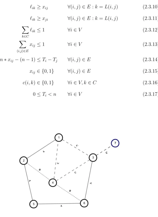
Mathematical Formulations
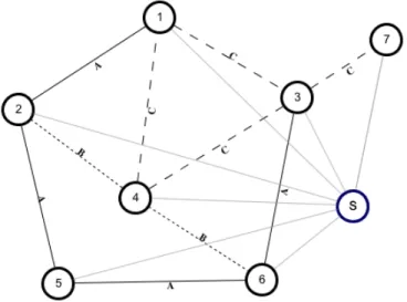
In this section we introduce two formulations for the MMP problem. The main difference between the two formulations is the technique used to obtain and count the connected substructure. In the former we use a set of flow constraints, in the latter we use the Miller-Tucker-Zemlin constraints [24].
The first mathematical model(M1 ) is modeled like a network flow problem. Given the colored and undirected graphG = (V, E, C), we build a new oriented and colored graphG0 = (V0, E0, C) derived from G such that V0 =V ∪{s} and E0 ={(i, j), (j, i) | (i, j) ∈ E} ∪ {(s, i) | i ∈ V }, where s is a new source node connected to each node in V . Since G0 is directed, we denote by δ+(i) and δ−(i) the forward and backward star of node i in G0. To each node of i ∈ V0 \ {s} is associated a request di = −1 (destination node) wile to the source node s is associated an offer equal to
n, ds = n, in order to satisfy the requests of destination nodes. No capacity to the
edges inside the graph is associated. Notice that every time an edge of δ+(s) is used, a new component ofG is generated. Whereas our aim corresponds to minimizing the number of connected component, we associate to each edge (s, i) ∈ δ+(s) a cost equal to 1 if the flow crosses it and zero otherwise. For the remaining edges inE0 the cost is equal to zero. Minimizing the cost needed to satisfy the requests of destination nodes means to minimize the number of used edges in δ+(s) and consequently the number of connected components of G. In order to guarantee that all connected components are monochromatic, we insert a constraint to ensure that in any solution all incident edges to the same node i have the same label.
Let xij be a variable representing the flow along the edge (i, j) ∈ E0, and let yi
is used and 0 otherwise. Finally, let us define the boolean variable`i,c whose value is
equal to 1 if exist at least ane edge with label c incident to node i and 0 otherwise
(P LF )z = min X i∈V0\{s} yi (2.3.1) with constraints: X (i,j)∈δ+(i) xij − X (k,i)∈δ−(i) xki =di ∀i ∈ V0\ {s} (2.3.2) Miyi ≥ xsi ∀i ∈ V0\ {s} (2.3.3) Mc,i`i,c ≥ X (i,j)∈δ+(i):L(i,j)=c xij ∀c ∈ L, ∀i ∈ V0\ {s} (2.3.4) Mc,i`i,c ≥ X (k,i)∈δ−(i):L(k,i)=c xki ∀c ∈ L, ∀i ∈ V0\ {s} (2.3.5) X c∈L `i,c ≤ 1 ∀v ∈ V (2.3.6) xij ≥ 0 ∀(i, j) ∈ E0 (2.3.7) yi, `i,c ∈ {0, 1} ∀i ∈ V0 (2.3.8)
Mi andMc,i represent the size of the maximum monochromatic connected
compo-nent containing the node i in G and the size of the maximum connected component whose color is c containing i respectively. Constraints (2.3.2) are the classical conser-vation flow constraints. The constraints (2.3.3) guarantee thatyi assume value equal
to 1 if the edge (s, i) is selected; the constraints (2.3.4) and (2.3.5) guarantee that the variable `i,c assume value equal to 1 if at least one edge (k, i) whose label is c
is selected and zero otherwise. Finally, constraints (2.3.6) ensures that all the edges incident to a node i have the same label.
M2. The next mathematical formulation M2, is very compact, and very easy to understand. This model selects the edges composing the solution. The boolean variable xij is equal to one if and only if the model selects the edge (i, j). To count
the number of connected components present in the solution, in order to describe the objective function an easy subtraction is used. Obviously if each connected component included in the solution is acyclic the number of components is equal ton−P(i,j)∈Exij
wheren = |V | (2.3.9). To ensure the subcycle elimination, the model uses the Miller-Tucker-Zemlin family constraints [24]. We use an integer variable Ti associated with
each nodes i ∈ V . The model is able to selects the edge xij if and only if Ti > Tj
(2.3.14). Now to finish this model, it is just necessary to ensure that no edges with different colors and incidents on the same vertex are selected at same time. We use the variable `ik to guarantee this property. `ik is equal to one if the model selects an
edge, incident on i ∈ V of color k ∈ C (2.3.10) (2.3.11). Using the variable `ik it is
easy to apply a limitation on the number of used color for edge (2.3.13).
z = min (n − X
(i,j)∈E
with the constraints: `ik ≥ xij ∀(i, j) ∈ E : k = L(i, j) (2.3.10) `ik ≥ xji ∀(i, j) ∈ E : k = L(i, j) (2.3.11) X k∈C `ik ≤ 1 ∀i ∈ V (2.3.12) X (i,j)∈E xij ≤ 1 ∀i ∈ V (2.3.13) n ∗ xij − (n − 1) ≤ Ti− Tj ∀(i, j) ∈ E (2.3.14) xij ∈ {0, 1} ∀(i, j) ∈ E (2.3.15) c(i, k) ∈ {0, 1} ∀i ∈ V, k ∈ C (2.3.16) 0≤ Ti < n ∀i ∈ V (2.3.17)
Figure 2.3: M1 resulting Graph.
Figure 2.5: M2 Solution.
2.4
Polynomial case
In this section we will study the relation between the complexity of our problem (MMP ) and the characteristics of the input instances. In particular we prove that is possible solve MMP in polynomial time on acyclic graphs. Obviously each connected component of an acyclic graph is a tree. The solution is created by combining the optimal solution of each connected component, still optimal for the original instance. For this reason in the following section we introduce a polynomial time algorithm (TreeSolver ) able to produce the optimal solution if the input graph is a tree.
Before describing the algorithm, we introduce some further definitions: Input Graph G(V, E, C).
• Let F (v) be the set of nodes adjacent to v with degree equal to 1, i.e. F (v) = {v0 ∈ V : (v, v0)∈ E, δ(v0) = 1}
equal to 1F (v, c) = {v0 ∈ F (v) : C (v, v0) =c}
• Let F0 be the set of nodes having only adjacent node with degree equal to 1,
i.e. F0 ={v ∈ V : |F (v)| = |δ(v)|}
• Finally, let F1 be the set of nodes having one adjacent node with degree greater
than 1, the father of v that is denoted by R(v), and all the remaining adjacent nodes with degree equal to one F1 ={v ∈ V : |F (v)| + 1 = |δ(v)| > 1}
TreeSolver
The idea at base of this algorithm is that we can select, iteration after iteration, edges surely included in an optimal solution. After a brief description of TreeSolver we present its pseudocode (2.6). Fixing a vertex randomly as root of this tree, we place the vertices position sorted by level, accord to the distance to the root. In level n we identify the leaves. Step by step, this algorithm selects a vertex at the level (n − 1), and for this vertex selects a subset of incident edges X. It inserts all the edges of X in the solution after it removes them from the input tree.
The first step of the procedure is to initialize the set Sol. In the second step start the main loop, now iteration by iteration a vertex v ∈ F1 is selected. It identifies c ∈ C, the color associated with the maximum number of edges in δ(v). Now we identify two different cases.
SolveTree 1: Sol ← ∅ 2: while ∃v ∈ F1do 3: c ← arg max l∈C |F (v, l)| 4: p ← R(v) 5: if |F (v, c)| > |F (v, C (v, p))| then {Case 1 } 6: Sol ← Sol ∪ {(v, v0) ∈ E : v0 ∈ F (v, c)} 7: V ← V \ (F (v) ∪ {v}) 8: E ← E \ δ(v) 9: else{Case 2 } 10: Sol ← Sol ∪ {(v, v0) ∈ E : v0 ∈ F (v, C (v, p))} 11: V ← V \F (v) 12: E ← E\{(v, v0) ∈ E : v0∈ F (v)} 13: end if 14: end while 15: if ∃v ∈ F0 then 16: c ← arg max l∈L |C(v, l)| 17: Sol ← Sol ∪ {(v, v0) ∈ E : L(v, v0) = c} 18: end if 19: return Sol Figure 2.6: TreeSolver
i.e.|F (v, c)| ≥ |F (v, l)| ∀ l ∈ C and |F (v, c)| > |F (v, C (v, R(v)))|. In this case all the edges (v, v0) with v0 ∈ F (v, c) are introduced in Sol and v and the nodes in F (v) are removed from the tree. In figure 2.7 the result of this step is shown. There is exactly one predominant color (figure 2.7a). Consequently, TreeSolver inserts in S the edges (v, v1), (v, v3) and (v, v4) and it removes the nodesv, v1, v2, v3, v4, v5 from the tree (figure 2.7b).
(a) (b) p v c2 c1 c2 c2 c1 c1 p v1 v2 v3 v4 v5
Figure 2.7: Case 1 of while loop.
• Case 2. There is no predominant color.
In this case it selects the color equal to C (v, R(v)). All the edges (v, v0) with v0 ∈ F (v, c) are introduced in Sol and the nodes in F (v) are removed from the
tree. In figure 2.8 the result of this step is shown. There are two predominant colors, c1 and c2 (figure 2.7a), but since C (v, p) = c1 the color c1 is selected. Consequently, TreeSolver inserts inS the edges (v, v2) and (v, v4) and it removes the nodesv1, v2, v3, v4, v5 (figure 2.8b).
(a) (b) p v c2 c1 c3 c2 c1 c1 p v c1 v5 v4 v3 v2 v1
Figure 2.8: Case 2 of while loop.
all the edges. Otherwise there is just a vertex v ∈ V0, in which case the algorithm computes the predominant color in v and it inserts in S the corresponding edges.
2.4.1
Solution’s Optimality
Using the induction, we will proving the solution’s optimality. The first step is to introduce a lemma. It will be used to ensure the termination of the algorithm: Lemma 2.4.1. The node v is an internal node if and only if it isn’t a leaf.
After each iteration of TreeSolverthe number of internal nodes in the tree is decreased by one or two units.
Proof Let v be the internal node selected at the generic iteration k of the al-gorithm. If we are in Case 1, we remove v and all the leaf nodes connected to v from the tree. In the resulting tree we have at least one internal node less, exactly v (Figura 2.7a), but if |δ(R(v))| = 1 we have removed two internal nodes. If we are instead in Case 2, the procedure removes all the leaf nodes connected to v from the tree. Now v is a leaf, and we have just removed an internal node (Figura 2.8b)).
(a) (b)
Figure 2.9: Base of the Induction
Theorem 2.4.2. Using a connected acyclic graph G(V, E, C), as input to the Tree-Solveralgorithm, produces a set of monochromatic connected components of cardinality equal to the optimal solution to the MMP problem.
Proof This proof is based on the induction method. The induction is defined on the number of internal nodes in G. The base of the induction is defined below, it is composed of two different cases.
1. Zero internal nodes
In this case we can have a graph composed by one node, or two nodes connected by an edge (Figura 2.9a). In both cases the optimal solution is equal to one. Step 15 of TreeSolver is able to find it.
2. One internal node (Figura 2.9b)
In this case the optimal solution is to select the most frequent color. Step 15 of TreeSolver is able to find it.
Using the inductive hypothesis we can assume that TreeSolver is able to produce the optimal solution in each graph with a number less than or equal to k of internal nodes. Now we try to prove that TreeSolver found the optimal solution in a graph with
Figure 2.10: Inductive step
k+1 internal nodes. Let v be the first node in G selected by TreeSolver(Figura 2.10a). After the first iteration, using the lemma 2.4.1 we can say that in the resulting graph G0, the number of internal nodes is decreased by one or two units. We can have two
cases:
C1 : v is present in the resulting graph (Figure 2.10b). C2 : v isn’t present in the resulting graph (Figure 2.10c).
We can analyze the two cases C1 and C2 separately.
C1: Let Sol∗ be an optimal solution for the input graph G. We can write: |Sol∗| = r + h − 1 where h is the number of components present in the optimal solution in the sub-tree rooted in v, and r is the number of components present in the optimal solution in the residual tree G0. Let S(G0) and S(Gv) be the solution computed by
the procedure respectively in residual tree G0 and in the sub-tree rooted in v. We can define p = |S(G0)| and q = |S(Gv)|. Using the inductive hypothesis we can
say that p ≤ r and taking into account the greedy choice of the procedure we can say that h ≤ q. Combining S(G0) and S(Gv) in a feasible solution of G we have
S(G) = S(G0)∪ S(G
The −1 depends on the color incident on v. In both solutions the color incident in v is the same and for this reason we can merge the two components including v in S(G0) and S(G
v).
C2 is in turn divided in two sub-case C2-a and C2-b.
• There exists an optimal solution on G that don’t use the edge (p, v).
Using the inductive hypothesis and taking into account the greedy choice of the procedure we can say that this procedure generates an optimal solution for the input graphG.
• All the optimal solutions on G use the edge (p, v). |Sol∗| = r + h − 1 , p = |S(G0)| and q = |S(G
v)|. Obviously h ≤ q and p ≤ r
but since the procedure doesn’t use the edge (p, v) then q < h. The solution produced by the procedure is S(G) = S(G0)∪ S(Gv) and |S(G)| = p + q <
r + h ⇒ p + q ≤ r + h − 1.
2.5
Genetic Approach
In this section we use a genetic algorithm to produce an heuristic solution for the NP-Hard instances of the problem. In particular we adapt the OMEGA (1) GA structure to the MMP problem. This algorithm is very similar to the version proposed in the first chapter moreover, the two problems are strictly related. Despite this similarity, for this particular problem the structure of the chromosome and the mutation function try to take advantage of the specific features of the problem.
2.5.1
The Chromosome
There exist two main parameters used to describe the chromosome, W and H. They are used to describe the maximum dimensions of the chromosome. W represents the width of the chromosome, in particular the maximum number of blocks. H represents the height of the chromosome, corresponding to the maximum number of elements for each block. To obtain an effective procedure, it is preferable to set the parameters according to the input instance. In the following experiments we have used: W ← |V |10 and H ← 3. chromosome 1 2 3 4 B1 B2 B2 B4 B5 B6 lunedì 26 ottobre 2009
Figure 2.11: MMP ’s chromosome structure
It is not the case that we choose H ← 3, in particular for the MMP problem we prefer to use a low value for H. The reason is that the block represents, for this problem, our choices for a specific vertex. In other words, the solution for this problem is characterized by a sequence of vertices touched by just one color and a sequence of key vertices touched by more than one color. The goal of this procedure is to identify the vertices that use more the one color in the final solution. In figure 2.11 is presented a chromosome composed of six blocks. Each block has a dimension
between one and four. Now we need an algorithm that takes a chromosome as input and produces a spanning tree as output. In figure 2.12 is presented an algorithm able to produce a spanning tree using a chromosome as input.
The algorithm builds the set Cost, associating to each edge a negative integer representing the occurrences of the label in the chromosome. In addition, for all the edges not presents in the chromosome, if they connect two vertices that are monochromatic in the chromosome, or are monochromatic with a vertex that is not present, it insert the edge as it is one time present in the chromosome.
After using a Minimum Weight Spanning Tree procedure (MST) it is possible to build the solution. The MST takes into account as cost for each edgee :Sol(L(e)) .
TreeCreator
INPUT: G(V, E, L) , chromosome c OUTPUT: Sol ∈ E Sapnning tree of G
1: Cost ← ∅
2: for all edge e ∈ c do
3: if ∃ (e, i) ∈ Cost then {Case 1 } 4: Cost ← {(e, i − 1)} ∪ Cost \ {(e, i)} 5: else{Case 2 }
6: Cost ← {(e, −2)} ∪ Cost 7: end if
8: end for
9: while is possible add edge to Cost do
10: select (v1, v2) ∈ E such that ∀((v1, v), i) ∈ CostL((v1, v)) = l for any v ∈ V i < 0
11: if ∀((v2, v), i) ∈ CostL((v2, v)) = l for any v ∈ V i < 0 then 12: Cost ← {((v1, v2), −1)} ∪ Cost
13: end if
14: if 6 ∃((v2, v), i) ∈ Cost for any v ∈ V i < 0 then 15: Cost ← {((v1, v2), −1)} ∪ Cost
16: end if 17: end while
18: Sol ← MST (G(V, E, L, Cost)) 19: return Sol
2.5.2
The Crossover
The crossover is the easiest function of OMEGA’s architecture. Basically the function takes as input two chromosomesc1, c2 and it produces as output the chromosome c3. The procedure randomly selects 50% of the blocks of c1 and c2, and it inserts the blocks into the new chromosome c3. In figure 2.13 is shown a graphical example.
chromosome 1 2 3 4 B1 B2 B2 B4 B5 B6 A C F F H B C chromosome A D I E F I A C B C chromosome 1 A C F C chromosome 2 D I I E A B Input: A D I E F I A C B C chromosome 1 A C F C chromosome 2 D I I E A B Selection: A D I E F I chromosome 1 chromosome 2 D I A B Selection: A D I E F I chromosome 3 D I A B Output: martedì 27 ottobre 2009 Figure 2.13: Crossover
2.5.3
The Mutation
There are three different kind of mutation MUT-ADD, MUT-DEL and MUT-CHANGE. The mutation operator randomly runs one of these three, if isn’t possible to use MUT-ADD or MUT-DEL it uses MUT-CHANGE.
Respectively the chances of selecting the operators are: 50%, 30%,20%.
another edge in the last position. Let (v1, v2) be the first edge of the block; the new edge is selected from the set of edges (v1, v) ∈ E.
• MUT-DEL randomly selects a block in the chromosome, and if its dimension is greater than one, it removes a random edge from the block.
• MUT-CHANGE randomly selects a block in the chromosome, randomly selects an edge from the block and replace it with a new edge. Let (v1, v2) be the first edge of the block; the new edge is selected from the set of edges (v1, v) ∈ E.
2.5.4
The Splitting Population Function
The Splitting Population Function (SPF) is used to partition the original population into k sub-populations. This procedure is totally random, and if h is the dimension of the original population, it produces k new populations, each one with a dimension equal to h
k. The aim of this procedure is to move the chromosomes present in a unique big population, into k different new populations.
2.5.5
The Fitness Functions
The fitness function takes in input a chromosomec, using the procedure 2.12 produce a spanning treeSP that is composed of |V |−1 edges of the original graph G(V, E, L). For each non-monochromatic vertex, it selects the most frequent color and it removes all the edges of different colors. The procedure returns the number of connected components produced by this process. Now we want to identify other fitness functions related to the first one. The technique is very easy. The procedure associates a penalty cost to a defined color on a defined vertex. If the dominant color of this
vertex is the forbidden color, an extra cost is added to the function. Usually the procedure identifies some good solutions in the current population and tries to forbid the selection of one or more used labels for particular vertices. The penalty cost is usualy greater than 1 and less than 3.
2.5.6
Pseudocode
BASIC-GA
INPUT: G(V, E, L) and Population P and Fitness function ft OUTPUT: Population P
1: Cost ← ∅
2: for it iterations do
3: for allc in P les the best tree do
4: select randomly c1 ∈ P such that ft(c) > ft(c1) 5: P ← (P \ {c}) ∪ {crossover(c1, c)}
6: end for
7: for allc in P les the best one do 8: P ← (P \ {c}) ∪ {mutation(c)} 9: compute ft(c)
10: end for 11: end for 12: return P
Figure 2.14: Basic Genetic Algorithm
2.6
Results
This section presents a preliminary test phase on small instances (15 nodes, num-ber of colors between 3 and 10 and graph density between 0.25 and 1). We solved the problem to optimality by means of the CPLEX solver using both the Single Commodity flow and the MTZ formulations and compared the obtained results with our OMEGA algorithm. While the complexity of the Single Commodity formulation
Instances
Flusso
MTZ
Genetic
Value
Time
Value
Time
Value
Time
15 25 3 1101
4
0,71
4
0,03
4
1,30417
15 25 3 1109
3
5.31
3
0,04
3
1,34739
15 25 3 1117
4
11.16
4
0,05
4
1,36868
15 25 3 1125
4
0,67
4
0,04
4
1,30625
15 25 3 1133
5
1.26
5
0,1
5
1,24156
15 25 10 1221
7
2,78
7
0,04
7
1,0552
15 25 10 1229
7
8.24
7
0,03
7
1,04701
15 25 10 1237
7
3.07
7
0,06
7
1,05988
15 25 10 1245
6
8.38
6
0,06
6
1,12753
15 25 10 1253
6
10.04
6
0,06
6
1,14058
15 1 3 1581
1
21.36
1
3,59
1
8,4705
15 1 3 1589
1
1.26
1
0,8
1
8,4547
15 1 3 1597
2
4320.14.24
1
2,95
1
8,51108
15 1 3 1605
2
4320.14.24
1
1,17
1
8,55474
15 1 3 1613
2
4320.14.24
1
2,23
1
8,45683
15 1 10 1701
2
2211.21.36
2
74,26
3
8,28533
15 1 10 1709
2
147,68
2
70,03
3
8,40188
15 1 10 1717
2
4320.43.12
2
71,91
2
8,45794
15 1 10 1725
2
4320.14.24
2
15,2
2
8,40143
15 1 10 1733
2
918.57.36
2
20,72
2
9,4352
OMEGA
INPUT: G(V, E, L)
OUTPUT: Sol ∈ E Sapnning tree of G 1: P OP = {P0, P1, . . . P10} set of populations
2: |P0| = h
3: |P1| = |P2| = . . . = |P10| = 0
4: while Not End Conditions do 5: BASIC-GA(G, P0, f0)
6: if new best solution in P0 then 7: set new best solution
8: end if 9: SPF(P0) =⇒ |P0| ' |P1| ' . . . ' |P10| ' h 10 10: for allP ∈ P OP do 11: BASIC-GA(G, P, frandom) 12: end for 13: P0⇐ P1∪ P2∪ . . . P10 14: P1⇐ P2⇐ . . . ⇐ P10⇐ ∅ 15: end while Figure 2.15: MMP OMEGA
grows significantly even on these small instances, the MTZ formulation has much bet-ter performances. Our OMEGA approach reaches the optimal solution value in most of the istances and differs at most of a value of 1 on the others, while still providing fast computational times.
Bounded Degree Spanning Tree
3.1
Introduction
In this chapter we focus our attention on telecommunication network problems, with emphasis on optical networks. These networks require specific constraints to be mod-eled in order to take into account their particular physical characteristics, such as the propagation of the light in the optical fiber. In particular, in an optical network, the wave division multiplexing technology allows to propagate different light beams on the same optical fiber, as long as they use a different fixed wavelength. In this kind of networks multicast technology permits to replicate the optical signal from one source to many destination nodes by means of a network device (switch ) that permits to replicate a signal, splitting light. Many applications, such as world wide web browsing, video conferences etc., require such a technology for efficiency pur-poses. Such application often require the individuation of connected sub-networks such as the spanning trees (ST). There are several variants of the ST problem that are useful to model problems arising in communication networks. For example, the network may be required to connect a specified subset of nodes (Steiner Tree Problem