DOI:10.1051/0004-6361/201526380 c ESO 2016
Astronomy
&
Astrophysics
Hi-GAL, the Herschel infrared Galactic Plane Survey: photometric
maps and compact source catalogues
First data release for the inner Milky Way: +68
◦≥
l
≥ −
70
◦?,??S. Molinari
1, E. Schisano
1, D. Elia
1, M. Pestalozzi
1, A. Traficante
2, S. Pezzuto
1, B. M. Swinyard
3,
A. Noriega-Crespo
4, J. Bally
5, T. J. T. Moore
6, R. Plume
7, A. Zavagno
8, A. M. di Giorgio
1, S. J. Liu
1, G. L. Pilbratt
9,
J. C. Mottram
10, D. Russeil
8, L. Piazzo
11, M. Veneziani
12, M. Benedettini
1, L. Calzoletti
13, 14, F. Faustini
14, P. Natoli
15,
F. Piacentini
16, M. Merello
1, A. Palmese
1, R. Del Grande
1, D. Polychroni
17, K. L. J. Rygl
18, G. Polenta
14,
M. J. Barlow
19, J.-P. Bernard
20, 21, P. G. Martin
22, L. Testi
23, 24, B. Ali
25, P. André
26, M. T. Beltrán
24, N. Billot
27,
S. Carey
28, R. Cesaroni
24, M. Compiègne
29, D. Eden
30, Y. Fukui
31, P. Garcia-Lario
13, M. G. Hoare
32, M. Huang
33,
G. Joncas
34, T. L. Lim
3, 13, S. D. Lord
35, S. Martinavarro-Armengol
19, F. Motte
26, R. Paladini
12, D. Paradis
20, 21,
N. Peretto
36, T. Robitaille
37, P. Schilke
38, N. Schneider
39, B. Schulz
12, B. Sibthorpe
40, F. Strafella
41,
M. A. Thompson
42, G. Umana
43, D. Ward-Thompson
44, and F. Wyrowski
45(Affiliations can be found after the references) Received 22 April 2015/ Accepted 10 February 2016
ABSTRACT
Aims.We present the first public release of high-quality data products (DR1) from Hi-GAL, the Herschel infrared Galactic Plane Survey. Hi-GAL is the keystone of a suite of continuum Galactic plane surveys from the near-IR to the radio and covers five wavebands at 70, 160, 250, 350 and 500 µm, encompassing the peak of the spectral energy distribution of cold dust for 8 <∼ T <∼ 50 K. This first Hi-GAL data release covers the inner Milky Way in the longitude range 68◦>
∼ ` >∼ −70◦in a |b| ≤ 1◦
latitude strip.
Methods. Photometric maps have been produced with the ROMAGAL pipeline, which optimally capitalizes on the excellent sensitivity and stability of the bolometer arrays of the Herschel PACS and SPIRE photometric cameras. It delivers images of exquisite quality and dynamical range, absolutely calibrated with Planck and IRAS, and recovers extended emission at all wavelengths and all spatial scales, from the point-spread function to the size of an entire 2◦× 2◦
“tile” that is the unit observing block of the survey. The compact source catalogues were generated with the CuTEx algorithm, which was specifically developed to optimise source detection and extraction in the extreme conditions of intense and spatially varying background that are found in the Galactic plane in the thermal infrared.
Results.Hi-GAL DR1 images are cirrus noise limited and reach the 1σ-rms predicted by the Herschel Time Estimators for parallel-mode obser-vations at 6000
s−1scanning speed in relatively low cirrus emission regions. Hi-GAL DR1 images will be accessible through a dedicated web-based image cutout service. The DR1 Compact Source Catalogues are delivered as single-band photometric lists containing, in addition to source posi-tion, peak, and integrated flux and source sizes, a variety of parameters useful to assess the quality and reliability of the extracted sources. Caveats and hints to help in this assessment are provided. Flux completeness limits in all bands are determined from extensive synthetic source experiments and greatly depend on the specific line of sight along the Galactic plane because the background strongly varies as a function of Galactic longitude. Hi-GAL DR1 catalogues contain 123210, 308509, 280685, 160972, and 85460 compact sources in the five bands.
Key words. dust, extinction – infrared: ISM – stars: formation – Galaxy: disk – methods: data analysis – techniques: photometric
1. Introduction
The Milky Way Galaxy, our home, is a complex ecosystem in which a cyclical transformation process brings diffuse baryonic matter into dense, unstable condensations to form stars. The stars produce radiant energy for billions of years before releasing chemically enriched material back into the interstellar medium (ISM) in their final stages of evolution.
Although considerable progress has been made in the past two decades in understanding the evolution of isolated dense ? Herschelis an ESA space observatory with science instruments pro-vided by European-led Principal Investigator consortia and with impor-tant participation from NASA.
?? The images and the catalogues are only available at the CDS via anonymous ftp tocdsarc.u-strasbg.fr(130.79.128.5) or via
http://cdsarc.u-strasbg.fr/viz-bin/qcat?J/A+A/591/A149
molecular clumps toward the onset of gravitational collapse and the formation of stars and planetary systems, much remains hid-den. We do not know the relative importance of gravity, turbu-lence, or the perturbation from spiral arms in assembling the diffuse and mostly atomic Galactic ISM into dense, molecular, filamentary structures and compact clumps. We do not know how turbulence, gravity, and magnetic fields interact on differ-ent spatial scales to bring a diffuse cloud on the verge of star formation. We still do not have a comprehensive quantitative un-derstanding of the relative importance of external triggers in the process, although available evidence suggests that triggering is not a major pathway for star formation (Thompson et al. 2012; Kendrew et al. 2012). We do not know how the relative roles played by these different agents changes from extreme environ-ments like the Galactic centre to the quiet neighbourhoods of the Galaxy beyond the solar circle.
Today, it is possible for the first time to engage with this ambitious challenge, thanks to a new suite of modern Milky Way surveys that provide homogenous coverage of the entire Galactic plane (hereafter GP) and that have already started to transform the view of our Galaxy as a global star-formation engine (see Molinari et al. 2014for a recent review).
The UKIDSS Galactic Plane Survey (Lucas et al. 2008) on the 4m UK Infrared Telescope on Hawaii covered the three near-IR photometric bands (J, H and K) to eighteenth magnitude, producing catalogues of over a billion stars. The unprecedented depth (fifteenth mag) and resolution (200) of the NASA Spitzer satellite’s GLIMPSE survey was the first to deliver a new global view of the Galaxy at wavelengths of 3.6, 4.5, 5.8, and 8.0 µm (Benjamin et al. 2005), until then only partially accessible from the ground and with imaging capabilities limited to resolutions of a few arcminutes, at best. The resulting catalogue of 49 mil-lion sources is dominated by stars and, to a lesser extent, by pre-main-sequence young stellar objects (YSOs), with the 8.0-µm channel also showing strong extended emission that probes the interaction between the UV radiation from hot stars and molecu-lar clouds. The Spitzer-MIPSGAL survey at 24 µm (Carey et al. 2009) enables much deeper penetration of the dense molecular clouds to reveal nascent intermediate and high-mass stars. These surveys were limited to the inner third of the Milky Way GP and were complemented by GLIMPSE360, which used Spitzer in its warm mission to complete the coverage of the entire GP at 3.6 and 4.5 µm, and by the WISE satellite (Wright et al. 2010), which, as part of its all-sky survey, is covering the entire GP (al-though at lower resolution than Spitzer) between 3 and 25 µm.
At far-infrared and millimetre wavelengths, AKARI sur-veyed the entire sky between 65 µm and 160 µm in 2006–2007. Its spatial resolution of between 10and 10.5 (Doi et al. 2016)
rep-resented an improvement by a factor ∼3 over that of IRAS, al-though still a factor ∼5 larger than Herschel. The Planck satel-lite (Planck Collaboration I 2011) also surveyed the entire sky at wavelengths between 350 µm and 1cm, but with a resolution >50, which is insufficient to resolve the complexity of the
ther-mal dust emission in star-forming clouds.
Only ground-based facilities can at the moment achieve reso-lutions below 10in the millimetre regime. The ATLASGAL sur-vey (Schuller et al. 2009) has used the 12 m APEX telescope in Chile to map the portion of the GP at longitudes between roughly +60◦and −60◦ at 870 µm, the JPS survey (Moore et al. 2015),
using the JCMT antenna in Hawaii, gives deeper coverage at somewhat higher resolution in the northern part of this same re-gion at 850 µm, while the Bolocam GPS covers the first quadrant at 1.1 mm (Aguirre et al. 2011). These (sub-)millimetre surveys provide a census of the cold and compact dust condensations that harbour star-formation; mass estimates require assumptions about dust temperatures that the single-band survey data them-selves cannot constrain, however.
Radio-wavelength continuum observations provide extinction-free views of bremsstrahlung radiation from ultra-compact HII (UCHII) regions and the ionised ISM in general. The 100. 5 resolution, 6 cm CORNISH survey used the
Very Large Array telescope to map the `= +10◦to+65◦section
of the GP at resolutions of ∼100 to ∼1000 (Purcell et al. 2013). The CORNISH-South extension of the project, carried out with the ATCA array, will complement this information for the corresponding region of the fourth quadrant, augmented with imaging in radio recombination lines.
This suite of continuum GP surveys is ideally complemented by a family of spectroscopic surveys of molecular and atomic emission lines. Kinematic information on the same dense clouds
traced by the thermal emission from cool dust can also be traced using molecular-line emission. The Galactic Ring Survey (GRS; Jackson et al. 2006), at 4600 resolution, uses the FCRAO 14 m antenna to map the 13CO (J = 1−0) transition in the range
15◦ <
∼ ` <∼ 56◦. The JCMT COHRS survey (Dempsey et al. 2013) covers essentially the same longitude range as the GRS, but in the CO (J= 3−2) line and at a spatial resolution of 1400.
Additional extensions to the GRS, in the first and second quadrants, toward the Galactic anticentre, also in 12CO (J = 1−0), have been carried out with the FCRAO (Heyer et al. 1998; Brunt et al., in prep.). The International Galactic Plane Survey (IGPS) has combined three interferometric 21 cm HI surveys at 45–6000 resolution. This combination provides an ideal tool to study the transformation of atomic into molecular gas in the spi-ral arms (e.g.McClure-Griffiths et al. 2001).
The coverage of the third and fourth quadrants in molecular lines is more sparse and less systematic. Together with targeted-source line surveys like MALT90 (Jackson et al. 2013), unbi-ased coverage of the plane is limited to the NANTEN survey (e.g.Mizuno & Fukui 2004), which is currently being improved with the NANTEN2/NASCO project, which still has limited (∼40) spatial resolution, however. Recent unbiased surveys with
the Mopra antenna in Australia (Burton et al. 2013;Jones et al. 2012) are starting to fill the gap with the data quality of the CO surveys in the northern portion of the GP. The SEDIGISM survey is currently being executed to map the fourth quadrant between ` = +18◦and ` = −60◦in13CO and C18O (J = 2−1) with the
APEX telescope.
The Methanol Multi-Beam survey (e.g.Green et al. 2012) is searching the plane for 6.7 GHz methanol maser emission us-ing the Parkes and ATCA telescopes. Methanol maser emission is characteristic of the early formation stage of massive stars; its association with cool dense clumps is a signpost for ongoing formation of massive stars and associated protoclusters in such objects. A more complete compilation of GP Surveys from the near-IR to the radio is provided in the review ofMolinari et al. (2014).
The Herschel infrared Galactic Plane Survey (Hi-GAL, Molinari et al. 2010b,a), carried out with the Herschel Space Observatory (Pilbratt et al. 2010), is the keystone in the arch of GP continuum surveys. With a full plane coverage of the thermal far-IR and submillimetre continuum in five bands be-tween 70 µm and 500 µm, ideally covering the peak of the spectral energy distribution (SED) of dust in the temperature range 8 K ≤ T ≤ 50 K, Hi-GAL delivers a complete census of structures containing cold dust, from the central molecu-lar zone to the outskirts of the Galaxy, enabling self-consistent determination of dust temperatures and masses. Thanks to its space-borne platform, the Herschel cameras do not suffer from the rapid atmospheric variabilities that limit ground-based sub-millimetre facilities. This allows full exploitation of the excel-lent sensitivity and stability of the infrared bolometric arrays to deliver exquisite-quality images that recover extended emis-sion from dust on all spatial scales. The ability of Herschel to recover multi-wavelength extended emission from the diffuse ISM, through dense filamentary structures, down to compact and point-like sources (Molinari et al. 2010a;André et al. 2010) are and will remain unparalleled in the coming decades.
Hi-GAL is delivering a transformational view of the com-plete evolutionary path that brings cold and diffuse interstellar material to condense into clouds and filaments that then fragment into protocluster-forming dense clumps. More than 50 papers have been published by the Hi-GAL consortium to date, based on Hi-GAL images and preliminary source catalogues, from
studies of the diffuse ISM (e.g.Bernard et al. 2010;Paradis et al. 2010; Compiègne et al. 2010; Traficante et al. 2014; Elia et al. 2014) to dense, large-scale filaments (Molinari et al. 2010a; Schisano et al. 2014; Wang et al. 2015), dust in HII regions (e.g. Paladini et al. 2012; Tibbs et al. 2012), clumps and mas-sive star formation (e.g.Elia et al. 2010,2013;Bally et al. 2010; Battersby et al. 2011; Mottram & Brunt 2012; Wilcock et al. 2012; Veneziani et al. 2013; Beltrán et al. 2013; Strafella et al. 2015; Traficante et al. 2015), Galactic central molecular zone studies (Molinari et al. 2011a;Longmore et al. 2012), triggered star formation (Zavagno et al. 2010), and finally dust around post-main-sequence objects (Umana et al. 2012; Martinavarro-Armengol et al., in prep.). More papers are in preparation by the Hi-GAL Consortium. Although basic Hi-GAL data have al-ways been open for public access through the Herschel Science Archive, we are now providing access for the larger commu-nity to the high-quality data products (maps and source catalogs) used internally by the Hi-GAL consortium.
In this paper we present the first public release of Hi-GAL data products (DR1). DR1 is limited to the inner Milky Way in the longitude range +68◦ ≥ ` ≥ −70◦ and latitude range
1◦≥ b ≥ −1◦, and consists of calibrated and astrometrically reg-istered images at 70, 160, 250, 350, and 500 µm, plus compact-source catalogues, delivered via an image cutout service pro-vided by the ASI Science Data Center1. We present and discuss the production methods and characterisation of the images and catalogues considered according to their band-specific proper-ties. A full systematic analysis of the physical properties of dense, star-forming and potentially star-forming condensations (reconstructed from the band-merged Hi-GAL photometric cat-alogues with augmented SED coverage from ancillary surveys from the mid-IR to the millimetre) will be presented in Elia et al., (in prep.). A first systematic analysis of far-IR properties of post-main-sequence objects based on the Hi-GAL catalogues is pre-sented in Martinavarro-Armengol et al. (in prep.).
2. Observations
The motivations and observing strategy adopted for the Hi-GAL Survey are described in detail in Molinari et al. (2010b). The complete survey was assembled in three instalments of observ-ing time granted in open time competition in each of the three calls issued during the Herschel project lifetime. Because of a clerical inconsistency in determining the duration time of the observations, a longitude range of about 6◦in extent in the outer Galaxy could not be executed in the observing time formally granted for the complete plane coverage, and director’s discre-tionary time was additionally granted to obtain the 360◦-wide
coverage. The total observing time amounted to slightly more than 900 h, making the full Hi-GAL survey the largest observ-ing program carried out by Herschel.
The Hi-GAL observations were acquired by subdividing the surveyed area into square tiles of ∼2◦.2 in size, to obtain
com-plete coverage of a |b| ≤ 1◦strip of the Galactic plane at 70, 160, 250, 350, and 500 µm simultaneously. Each tile was observed with the PACS (Poglitsch et al. 2010) and SPIRE (Griffin et al. 2010) cameras in parallel mode (pMode), specifically designed to optimise data acquisition for large-area multi-wavelength sur-veys. In pMode the PACS and SPIRE cameras are used simulta-neously, effectively making Herschel a five-band imaging cam-era spanning a decade in wavelength. Since the fields of view of the PACS and SPIRE cameras are offset by ∼200in the plane of
1 Accessible from the VIALACTEA project portal at http:// vialactea.iaps.inaf.it
the sky, slight oversizing of the individual observing tiles was needed to ensure that a 2◦× 2◦area was covered in all five
pho-tometric bands.
As the bolometers that constitute the elemental pixels of the PACS and SPIRE arrays are differential detectors known to be affected by slow thermal drifts with typical 1/ f frequency be-haviour, each tile was observed in two independent passes with nearly orthogonal scanning directions. Individual astronomical observation requests (AORs) were concatenated in the Herschel observation planning tool (HSpot) so that the two scanning passes were executed immediately one after the other for each tile. This strategy was chosen so that a given position in the sky was observed by as many pixels as possible and in different scan-ning directions, producing the degree of redundancy needed to beat down the correlated and uncorrelated 1/ f noise of single detectors, thereby allowing recovery of all the emission at the largest possible spatial scales. The approach was also designed to perfectly couple to the data processing and map-making pipeline specifically developed for the Hi-GAL project (see Sect.3).
The satellite scan speed in pMode was set to its maximum value of 6000per second, with a detector sampling rate of 40 Hz for PACS and 10 Hz for SPIRE. The spatial sampling is there-fore 1.500and 6.000for PACS and SPIRE, respectively, enough to Nyquist sample all the nominal diffraction-limit beams ('[6.0, 12.0, 18.0, 24.0, 35.0]00at [70,160, 250, 350, 500] µm, respec-tively). However, because of the limited transmission bandwidth, the PACS data were co-added on-board Herschel, with a com-pression of eight and four consecutive frames at 70 and 160 µm, producing an effective spatial sampling of 1200and 600at 70 and
160 µm respectively. Therefore, in pMode, the PACS beams are not Nyquist sampled and the resulting point-spread functions (PSFs) are elongated along the scan direction with a measured size of 5.800× 12.100and 11.400× 13.400at 70 µm and 160 µm,
respectively (Lutz 20122).
TableC.1summarizes a few details of the observations. Col-umn 1 is an assigned field name for each tile, Cols. 2−5 report the approximate coordinates of the tile centre, Cols. 6 and 7 in-dicate the date of the observation for each tile, both in standard format and in OD number (observation day, starting from date of launch), Cols. 8−10 report the start time (UT) of the tile in the nominal and orthogonal scan direction (see below), together with the associated observation identification (OBSID) number uniquely attached to each scan observation.
SPIRE was used in bright-source mode in the three tiles of the survey closest to the Galactic centre (roughly centred at lon-gitudes+2◦, 0◦and −2◦). This was done to avoid the widespread
saturation and non-linearities in the detector response that are otherwise likely to occur on the extraordinarily strong back-ground emission in that region. In this observing mode, the lim-ited 12-bit dynamical range of the analog-to-digital converters in the detector chains is centred around higher-than-nominal cur-rent values. In this way, saturation is avoided at the cost of greatly decreased sensitivity. In bright-source mode SPIRE is much less capable of detecting intermediate and low-flux com-pact sources (see Fig.20, last three panels).
3. Production of the photometric maps
The data reduction was carried out using the ROMAGAL data-processing software described in detail inTraficante et al. (2011). In short, the pipeline uses standard Herschel interactive
2 http://herschel.esac.esa.int/twiki/pub/Public/
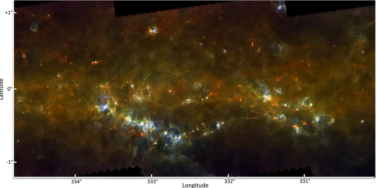
333°# 332°# 331°# 334°# '1°# 0°# +1°# La, tu de # Longitude#
Fig. 1.Three-colour image (blue 70 µm, green 160 µm, red 350 µm) of a three-tile mosaic field around 330◦<
∼ ` <∼ 335◦.
processing environment (HIPE) (Ott 2010) processing up to level 0.5, where the signal from individual detectors is photometri-cally calibrated and each detector has its sky position assigned. Subsequent steps in the data reduction were carried out using a dedicated pipeline written by the Hi-GAL consortium. Fast and slow detector glitches arising from particle hits onto the detec-tors are identified and the affected portions of the data are flagged in each detector’s time ordered data (TOD). Slow detector drifts arising from 1/ f noise are estimated and subtracted; for PACS, the drifts are estimated at subarray level as each 16 × 16 array matrix shares the same readout electronics. The core of the map-making implements a generalised least-squares (GLS) algorithm that is ideally designed to use redundancy to minimise resid-ual uncorrelated 1/ f detector noise by filtering in Fourier space (Natoli et al. 2001). To deliver optimal results, the code (i.e. each GLS-based code) requires that the detector noise properties are regularly sampled in time over the entire duration of the obser-vations. For this reason, we implemented a pre-processing stage where the sections of the TOD flagged as bad data (e.g. due to a glitch removal or signal saturation) are replaced with artificial samples in which the data are set to 0, but where the noise is added using a constrained noise realisation using the noise fre-quency properties estimated from valid data immediately before and after the flagged section.
The pixel sizes of the ROMAGAL maps account for the larger-than-nominal PACS PSFs and are set to [3.2, 4.5, 6.0, 8.0, 11.5]00 at [70, 160, 250, 350, 500] µm respectively. This choice represents a good compromise between the need to sample the PSF as also determined for point-like objects in Hi-GAL maps with at least three pixels, while avoiding (for PACS 70 µm and 160 µm) excessively small pixels in which the hit statistics of the detector sampling are too low, resulting in increased pixel-to-pixel noise. For the PACS bands this arises because the Her-schelscanning strategy in pMode implements an on-board frame co-adding (see Sect.2), resulting in an effective decrease in sam-pling rate. The pixel size of the images is therefore such that the beam FWHM is sampled with three pixels for the three SPIRE
bands and with 2.66 pixels in the PACS bands. Saturated pixels in the maps are a consequence of signal saturation for all TODs covering the specific pixel, which is due to the necessary limita-tions in the dynamical range of DAC converters at the detection stage. A list of locations where saturation is reached is reported in AppendixB.
It is clearly not possible to report even in electronic form the complete list of images for all wavelengths and all the tiles of Table C.1 in this paper. We choose here to show only one figure (Fig.1) as a three-colour image of a three-tile mosaic in the longitude range 330◦ <∼ ` <∼ 335◦to set the framework for the subsequent sections (see Sects. 4 and 5.1), describing the properties of the compact-source catalogues. The maps deliver a stunning view of the GP at all Hi-GAL wavelengths with a detail that is unattainable from any ground-based millimetre-wave fa-cility now and in the foreseeable future. Extended emission with at least two orders of magnitude dynamical range in intensity is retrieved at all spatial scales from the most compact objects to the extent of the entire tile. We show in the next sections that compact sources within these multiple complex, extended struc-tures have a very low peak-to-background contrast ratio (gener-ally below 1). This makes the detection and flux computation of compact sources an extremely complex task, where it is in par-ticular difficult to identify a figure of merit that can be used to unambiguously distinguish reliable from unreliable sources.
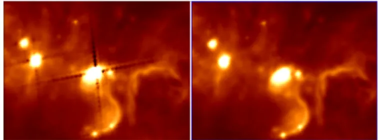
The pipeline is augmented with a module specifically devel-oped by the Hi-GAL team to compensate for the high-frequency artefacts that the GLS map-making technique used in ROMA-GAL (as in many other approaches, like MadMap or Scanamor-phos) is known to introduce to the maps, namely crosses and stripes corresponding to the brightest sources. The left panel in Fig.2 shows a typical example of these features that are intro-duced by the noise filter deconvolution carried out by the GLS map-maker in Fourier space when the flux is strongly varying with position, as is the case for point-like sources. We find that the minimum within a negative cross feature is proportional to the peak brightness of the source and amounts to ∼2.5% of this
Fig. 2.Left panel: particulars of a point source as reconstructed by the ROMAGAL map-making for PACS at 70 µm; the typical cross feature introduced by the GLS map-maker when performing the noise filter de-convolution in Fourier space over strongly varying signal (as is the case for point-like sources) is clearly seen (image in log scale). The mini-mum within the negative cross scales as ∼2.5% of the peak source flux. Right panel: same as left panel with the same scale and colour stretch, but after applying the correction devised byPiazzo et al.(2012). The angular extent of the region imaged is ∼60
× 40 .
value. It is therefore not a strong effect in principle, but it can be quite annoying for relatively faint nearby objects and for the determination of the surrounding diffuse emission; it is also aes-thetically undesirable.
To correct for these effects, which are particularly visible in the PACS 70-µm, and to a lesser extent, in the 160-µm images, a weighted post-processing of the GLS maps (WGLS,Piazzo et al. 2012) was applied to finally obtain images from which these artefacts are removed (right panel in Fig.2).
3.1. Noise properties of the Hi-GAL maps
To characterise the noise properties of the Hi-GAL DR1 maps, we considered all the tiles in each band, locating and analysing those map regions where the lowest signal is found. This was done by computing the pixel brightness distribution and select-ing pixels where the brightness was below the lowest 10 per-centiles. We subsequently considered always for each tile and each band separately only those pixels that formed connected areas with at least 100 pixels each. In these we computed the median of the brightness and the mean of its rms. These quanti-ties are reported in Fig.3as full and dashed lines as a function of Galactic longitude. The figure reports for each band the dis-tribution of the lowest brightness levels and the corresponding rms found in each tile. The coloured ticks on the right margin of the figure represent the 1σ brightness sensitivities in MJy/sr pre-dicted by the PACS and SPIRE time estimator for the Hi-GAL observing strategy, with two independent orthogonal scans taken in parallel mode at a scanning speed of 6000s−1.
Brightness levels are always well above the instrument sensi-tivities, showing that even in the faintest regions mapped by Hi-GAL, we are limited by cirrus brightness and cirrus noise emis-sion by big grains (Desert et al. 1990) for λ ≥ 160 µm, except perhaps at the outskirts of the Hi-GAL DR1 longitude range, where the minimum signal rms is close or equal to the predicted detector noise. An exception is the 70-µm emission, where the brightness of the diffuse cirrus that dominates at longer wave-lengths drops significantly (Bernard et al. 2010). The 70-µm brightness levels reach (or cross) the respective rms values much earlier, moving away from the Galactic centre, than in the other bands. The fact that the most intense emission is reached at 160 µm and then decreases toward 500 µm is in excellent agree-ment with expectations for diffuse, optically thin cirrus dust at
Fig. 3.Distribution as a function of Galactic longitude of the median
brightness (full lines) and its rms (dashed lines) in regions within each Hi-GAL tile where the brightness levels are below the 10 percentiles of the brightness distribution for that tile. Hi-GAL bands are colour-coded as follows: blue for PACS 70 µm, cyan for PACS 160 µm, green for SPIRE 250 µm, yellow for SPIRE 350 µm, and red for SPIRE 500 µm. Ticks on the right margin of the figure mark the values of the theoret-ical sensitivities predicted by the official PACS/SPIRE time estimator (available in HSpot) for observations in pMode with 6000
s−1scanning speed.
temperatures 16 K <∼ T <∼ 20 K, as determined byParadis et al. (2010) from detailed modelling of Hi-GAL data in selected re-gions of the GP.
It should be noted that the Hi-GAL ROMAGAL pipeline used for DR1 is successfully delivering the PACS and SPIRE predicted sensitivities with the very bright and complex ISM emission on the GP, while preserving in the data processing chain the signal at all spatial scales with no spatial scale filtering.
3.2. Astrometric corrections
Although the map-making algorithm was run for each tile using the same projection centre for all bands, the PACS and SPIRE maps are slightly misaligned, possibly due to a residual uncal-ibrated effect in the basic astrometric calibration that is carried out in the HIPE environment. Excellent map alignment is es-sential to generate products such as column-density maps (e.g. Elia et al. 2013) or to positionally match source counterparts at different wavelengths.
As the images obtained with the same instrument (PACS or SPIRE) are internally aligned, we initially aligned the PACS 70 µm images to match the astrometry of the Spitzer/MIPSGAL images at 24 µm. This has the advantage that the two instru-ment/wavelength combinations deliver the same spatial resolu-tion. The astrometric accuracy of the MIPSGAL images with respect to higher resolution IRAC and 2MASS is better than ∼100 on average (Carey et al. 2009).
For each tile, we visually selected a number of sources across the maps (typically more than six) that appear relatively isolated and compact both at 24 and 70 µm. The implicit assumption is that the two counterparts are the same physical source. This is reasonable as long as we avoid selecting sources in relatively crowded star-forming regions where sources in different evolu-tionary stages (and hence intrinsically different SED shapes) are generally found. We extracted the selected sources in both im-ages and determined an average [δl, δb] shift to minimize the
offsets between the positions of the selected sources in the 24-µm and 70-µm maps. This mean shift correction was then applied to the astrometric keywords in the FITS headers of the PACS maps. The SPIRE maps were aligned by bootstrapping from the aligned PACS images. For each tile we selected a number of sources that appeared compact and isolated both in PACS 160 µm and SPIRE 250 µm. In a similar way to the alignment of the 70-µm PACS images, we extracted the selected sources in both maps and compared the source positions in the two bands to determine an average shift that minimizes the positional dif-ferences. This average shift was then applied to correct the as-trometric keywords in the FITS headers of all SPIRE maps.
The corrections estimated for each tile are shown in Fig.4 for PACS (cross signs) and SPIRE (triangles) images, taking the Spitzer/MIPSGAL images as a reference. Corrections can be as large as 600in absolute terms, meaning they are particularly
sig-nificant for the PACS 70-µm band where they can reach about two-thirds of the image reconstructed FWHM beam width. The outlier point at the top right corner of the plot corresponds to the tile centred at ` = 299◦, which was taken during the Herschel performance verification phase. The Herschel astrometric accu-racy evolved throughout the mission because sources of errors in the star trackers and in general in the pointing reconstruction have been isolated and recovered. One of the main problems up to OD 320 were the speed bumps that caused large variations in the scanning speed of the telescope. These bumps occurred when a tracking star passed over bad pixels of the optical telecope’s CCD. This effect was corrected for by lowering the operational temperature of the tracking telescopes. In general, the astromet-ric accuracy up to OD 320 was better than 2 arcsec, but outliers at more than 8 arcsec were observed (for a detailed report on the Herschelastrometric accuracy seeSánchez-Portal et al. 2014).
The error bars in Fig.4represent the rms of the source co-ordinates used to estimate the offset corrections with respect to their mean value. The distribution of these values is reported in the lower panels of Fig.4; they are centred around the median values [∆GLON, ∆GLAT] = [000. 9, 000. 8] for the PACS images
(lower left panel of Fig.4), and [100. 7, 100. 6] for the SPIRE
im-ages (lower right panel), and may be considered an estimate of the typical residual uncertainty of the source coordinates. These amount to ∼ 10% of the PSF FWHM as estimated from compact sources in the images. It is interesting to note that there are a few outliers in the distributions, particularly apparent for the PACS shifts, but even for their maximum values they are below half of the PACS beam at 70 µm. As mentioned at the beginning of the section, an additional average 100uncertainty should be added in quadrature to account for the MIPSGAL pointing accuracy.
3.3. Map photometric offset calibration
Although the PACS and SPIRE images are calibrated internally in Jy/pixel and Jy/beam, respectively, their zero point level is not. To bring the images to a common calibrated zero level, an offset was therefore applied to the maps. The photometric off-sets of the Hi-GAL maps were determined through a comparison between the Hi-GAL data and the Planck and IRIS (improved reprocessing of the IRAS survey) all-sky maps, following the procedure described inBernard et al.(2010). We smoothed the Herschelmaps to the common resolution of the IRIS and Planck high-frequency maps of 50and projected them into the HEALPix pixelisation scheme (Górski et al. 2005) following the drizzling procedure described in Paradis et al. (2012), which preserves the photometric accuracy of the input maps. These smoothed
Fig. 4.Top panel: astrometry shifts in Galactic longitude (x axis) and
latitude (y axis), estimated for each tile in arcseconds. Crosses are for PACS tiles while triangles are for SPIRE tiles. The error bars represent the rms of the source coordinates used to estimate the offset corrections with respect to their respective mean value. Bottom panels: histograms of the rms of the longitude (full lines) and latitude (dashed lines) shifts estimated for PACS (left panel) and SPIRE (right panel).
Hi-GAL maps are compared with the IRIS and Planck all-sky maps (hereafter called “model”).
To make this model, we used the IRIS maps projected into HEALPix taken from the CADE web site3and the Planck maps shown in Planck Collaboration IX(2011). Since the Herschel, Planck,and IRAS photometric channels are different, the com-parison requires frequency interpolation with differential colour correction and the use of a model. We predicted the shape of the emission spectrum in each pixel using the DustEM4 code (Compiègne et al. 2011), computed for an intensity of the ra-diation field best matching the dust temperature, derived from the combination of the IRIS 100-µm and the Planck 857-GHz
3 http://cade.irap.omp.eu
4 Seehttp://dustemwrap.irap.omp.eu/andhttp://www.ias.
and 353-GHz maps. The dust temperature assumed is that of Planck Collaboration IX(2011) with the standard dust distribu-tion of Compiègne et al.(2011). For a given PACS or SPIRE band, the model was normalized to the data at the IRAS or Planck band at the nearest frequency to the considered Her-schelband, and a predicted 50resolution model image was con-structed. These nearest frequencies are the IRAS 60-µm and Planck857-GHz bands for the PACS 70-µm and 160-µm bands, respectively, and the Planck 857-GHz, 857-GHz, and 545-GHz bands for the SPIRE 250-µm, 350-µm, and 500-µm bands, re-spectively. In this process, the differential colour correction be-tween IRAS or Planck and the Herschel band under consid-eration was also taken into account using the spectral shape predicted by the model on a pixel-by-pixel basis.
This resulting model image was compared with the smoothed Hi-GAL data through a linear correlation analysis, the intercept of which provides the offset level to be added to the Herschel data to best match the IRIS and Planck data. This analysis also provides gain corrections (i.e. a slope of unity between the data and the model), but these are well below the cumulative relative uncertainties in the datasets used and in the dust modelling assumptions, and within 10%, on average, in all bands. The standard Herschel photometric calibration was there-fore assumed, and no additional gain corrections were applied. We also note that the Planck data used do not have the same absolute calibration as the publicly available version. A forth-coming processing of the Hi-GAL data will use the latest Planck calibration and will allow for a global gain correction.
4. Generation of photometric catalogues from Hi-GAL maps
In comparison to the ground-based submillimetre-continuum surveys, the Herschel instruments do not suffer from the need to correct for varying atmospheric emission and absorption, allowing recovery of the rich and highly structured large-scale emission from Galactic cirrus and extended clouds. Such variable and complex backgrounds, however, severely hin-der the use of traditional methods to detect compact sources based on the thresholding of the intensity image. Such meth-ods are widely used by large-scale millimetre and radio sur-veys from ground-based facilities, such as the Bolocam GPS (Rosolowsky et al. 2010), CORNISH (Purcell et al. 2013), or ATLASGAL (Contreras et al. 2013), where diffuse emission is filtered out either by atmospheric variation correction or the in-strumental transfer function. The possibility of processing Her-schelimages using high-pass filtering was discarded for various reasons. First of all, it would be difficult to choose a threshold in spatial scale. Dust cores and clumps are compact but, depend-ing on their distance and physical scale, may not be point-like (i.e. unresolved). A spatial filtering scale threshold too close to the PSF will remove power from compact but resolved sources, while a threshold high enough to ensure that no power is re-moved from scales corresponding to two to three times the PSF will prove ineffective to improve source detection in crowded fields. A second reason is that any high-pass spatial filtering will introduce negative lobes with intensities proportional to the brightness of the extended emission, severely hindering the de-tection of faint sources that fall within those features.
In a previous work, Molinari et al. (2011b) introduced a new method to detect sources and extract their fluxes tailored to the case of the complex and structured background present in IR/sub-mm observations. With respect to other popular
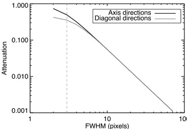
1 10 100 FWHM (pixels) 0.001 0.010 0.100 1.000 Attenuation Axis directions Diagonal directions
Fig. 5.Relative attenuation of the peak intensity induced by the
deriva-tive filtering as a function of the scale of the structure. The diagonal directions have been divided by
√
2 to take the longer distance along the diagonals with respect to the normal axis into account. For scales longer than ∼6 pixels, the damping increases as a power -law function with an exponent −2. The dark grey dashed line refers to the typical size in pixels of the PSF in Hi-GAL maps.
algorithms, the C
u
TEx
5 photometry code, standing for CUrva-ture Thresholding EXtractor, adopts a different design philoso-phy, looking for the pixels in the map with the highest curvature by computing the second derivative of the map. All the clumps of pixels above a defined threshold are analysed, and those larger than a certain area are kept as candidate detections. The pixels of the large clumps are checked to determine enhancement of cur-vature in the case of multiple sources. For each detection, an esti-mate for the size of the source is determined by fitting an ellipse to the positions of the minima of the second derivative in each of the eight principal directions. The output fluxes and sizes are determined by simultaneously fitting elliptical Gaussian func-tions plus a second-order 2D surface for the background. All the sources whose detected centres are closer than twice the instru-mental PSF are fitted together to separate their fluxes.The Gaussian fitting was carried out for each source by con-sidering a fitting window centred on each source and with a width of three times the instrumental PSF to ensure that we in-cluded sufficient space surrounding the source for a reliable es-timate of the background. This has the drawback that the pixels used to constrain the background are numerically predominant with respect to the pixels characterising the source; to counter-balance this effect, the pixels located within a distance equal to the initial guess-estimated source size from the source position are given a higher weight in the fit.
4.1. Characterisation of the photometric algorithm
CuTEx, as a derivative-based detection algorithm, acts as a high-pass spatial filter; however, contrary to simple median or box-car filtering, derivative filtering has inherent multiscale capabil-ities by selectively filtering out the larger of the spatial scales in a continuous way with higher efficiency. This behaviour is shown in Fig.5, where we report for Gaussians with increas-ing widths the ratio between the second derivative image and the original one at the peak position as a function of the spatial scale expressed in pixels. The results shown are obtained on a
5 See http://herschel.asdc.asi.it/index.php?page=
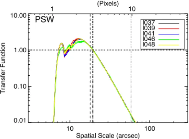
10 100 Spatial Scale (arcsec) 0.01 0.10 1.00 10.00 Transfer Function 1 (Pixels) 10 PSW l037 l039 l041 l046 l048
Fig. 6.Ratio between the power spectrum of the derivative images
(av-eraged over the four directions) computed by CuTEx and the power spectra of the intensity image for SPIRE 250 µm as a function of spa-tial scale expressed in arcseconds and in pixels (upper x axis). Each colour corresponds to a different map; black to the l037, red to the l039, blue to the l041, green to the l046, and yellow to the l048 field. All the functions overlap for scales larger than the PSF, indicated as a dark grey dashed line, and decrease following a power law with an ex-ponent ∼–3.9. The black dot-dashed line indicates the scale at which the transfer function is equal to unity. Scales smaller than this result in an overall amplification in the second derivative maps. The light grey dot-dashed line traces the scale above which the extended sources be-come confused with the background in the derivative image. This value corresponds approximately to ∼3 times the PSF. Similar plots are found for other wavelengths, and the functions completely overlap when the spatial scales are expressed in pixels.
simulated image where the FWHM of the PSF is sampled by three pixels, and therefore is a general result applicable to any map that shares this characteristic, like the Herschel maps we present here. Figure5 shows that the peak intensity of a point-like source, with a FWHM of ∼3 pixels (i.e. 1 PSF), is damped in the second derivative image to ∼40% of its original value, while an extended source with FWHM of ∼7.5 pixels (i.e. 2.5 × PSF) and the same peak intensity is damped to ∼10% of the origi-nal value. In other words, a point source in the intensity map that is ten times fainter (contrast 0.1), for instance, than the sur-rounding background, with a typical scale of order 15 pixels, that is, 5 × PSF, will appear in the derivative map as ∼1.7 times brighter than the background (contrast 1.7). Given the trend in Fig.5, where attenuation decreases following a power-law be-haviour with an exponent –2, it is then possible to detect sources with less favourable contrast the larger the background typical scale. Clearly, the method has the inherent drawback of being most effective for more compact objects (see below).
To confirm the performances of CuTEx’s derivative operator for real maps, we computed the power spectrum of the second derivative image for each map, averaging the spectra obtained for each derivative direction. We then divided each derivative power spectrum by the power spectrum of the parent intensity image. These ratios are proportional to the module square of the trans-fer function of the derivative operator used by CuTEx. Figure6 shows these ratios for five different maps (indicated with differ-ent colours in the figure) for 250-µm observations. Similar plots are found for the other wavelengths, where the only difference is a shift in angular spatial scale that is due to the different pixel scales. The scale in the upper x axis is in pixels and insensitive to the specific pixel angular scale.
Several conclusions can be drawn from the analysis of these functions. First, the transfer function is the same, regardless of the mapped region, for scales larger than the PSF. Second, the damping introduced by the derivative operator found in Fig.5is also confirmed for real maps. From an investigation of a sample of very extended sources in the Hi-GAL maps, we estimated that CuTEx is not able to recover most of the sources with sizes larger than three times the PSF (see also Fig.18), being completely in-sensitive to any source larger than ∼5 times the PSF. The third conclusion resulting from Fig.6is that the derivative filtering in-troduces an amplification for scales smaller than the PSF. This means that any pixel-to-pixel noise present in the intensity map is increased in the second derivative maps. Slight differences be-tween the different tested fields are only visible at scales below the PSF (the dashed line in the figure) but are not relevant for the detection of real sources. To quantify this increase, we tested the effect of the derivative operator on pure Gaussian noise maps and found that the noise in the second derivative follows the same distribution, with a standard deviation 1.13 times the initial one. This behaviour is not unexpected because of the linearity prop-erties of the derivative filtering.
4.2. Choice of the extraction threshold
In similar way to source extraction performed on images of surface brightness distribution, it is useful to set an extraction threshold as a function of the local curvature rms instead of adopting a constant absolute value. In this way, the depth of the extraction is adapted to the complexity of the morphological properties and to the intensity of the background that constitutes the dominant flux contribution in the far -infrared toward the GP. Although the adoption of a detection threshold in the second derivative image is certainly less intuitive than adopting a thresh-old on the flux brightness map, we have shown above that the noise statistical properties do not change from flux maps to flux curvature maps (except for a small increase in the width of the noise distribution), so that the notion of a threshold that adapts to the local noise properties can also be applied to detection on the curvature images.
The choice of an optimal source extraction threshold al-ways results from a compromise between the need to extract the faintest real sources and the need to minimize the number of false detections. Pushing the detection threshold to increas-ingly lower values to extract ever fainter sources is of course of minimal use if the majority of these faint extracted sources have a high probability of being false positives, therefore consider-ably limiting the catalogue completeness and reliability. Unfor-tunately, there is no exact way to control the number of false pos-itives extracted from real images because there is no control list for real sources present, so that a number of a posteriori checks are needed to determine this optimal threshold value.
The procedure we adopted to estimate the optimal extraction threshold is to make extensive synthetic source experiments to characterise the flux completeness levels obtained for different C
u
TEx
extraction thresholds σcin all five Hi-GAL photometricbands, where σcis in units of the rms of the local values of the
second derivatives of the image brightness averaged over four directions (seeMolinari et al. 2011b).
As it is clearly impractical to make these studies over the entire set of Hi-GAL tiles, we chose three tiles at Galactic lon-gitudes of 19, 30, and 59 degrees that are representative of the widely variable fore-to-background conditions that can be found
over the entire survey. For each of these tiles and for each ob-served band, hundreds of synthetic sources were injected at dif-ferent flux levels. We then ran C
u
TEx
for a set of extraction thresholds σc from 3 to 0.5, estimating for each threshold theflux for which 90% of the synthetic sources were successfully recovered. We verified that, for each of the three tiles, the 90% completeness fluxes decrease with decreasing extraction thresh-old. For the three SPIRE bands, we see that this decrease flat-tens, starting at σc∼ 2, meaning that we do not gain in depth of
extraction at lower thresholds. We emphasise that our artificial source experiments provide the same optimal value for the ex-traction threshold independently of the tile used, in spite of the very different properties of the diffuse and structured background exhibited by the Hi-GAL images in the longitude range covered in DR1. This is a convenient feature of the detection method, which is clearly able to deliver similar performances with very similar parameters in widely different fields. We then adopted σc= 2 as the extraction threshold for the SPIRE bands.
For the PACS 70-µm and 160-µm bands, the decrease of the 90% completeness fluxes continues below σc= 2. This apparent
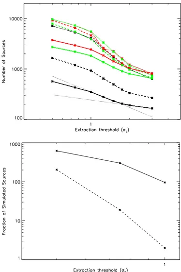
gain in the number of reliable sources detected at increasingly lower thresholds is probably due to increasing numbers of false-positive detections. We characterise the effect of false positives by evaluating the number of extracted sources in the different bands as a function of the extraction threshold. Figure7top re-ports the number of sources detected in the three tiles (indicated by the different colours) at 70, 160 and 250 µm (solid, dashed, and dotted lines) as a function of the extraction threshold. The figure shows that in all cases the N-σcrelations tend to become
steeper below σc ∼ 2; we emphasise this in Fig.7in one case
by fitting two power laws to two portions of the N-σc for the
70 µm case of ` = 59◦ (the two thin dotted lines). A similar behaviour is exhibited for all the other cases, and we interpret this increase of rate in detected sources for σc≤ 2 as an
indica-tion of increased contaminaindica-tion of false detecindica-tions. It is, strictly speaking, impossible to verify this claim on real images because we do not have a truth table for the sources that are effectively present. We then used a subset of the extensive simulations per-formed inMolinari et al.(2011b), where we presented and char-acterised the CuTEx package; the bottom panel of Fig.7reports the number of true detected sources (full line) and the number of false positives (dashed line) as a function of the extraction threshold for a simulation of 1000 synthetic sources (that were reported in the top-left panel of Fig. 7 inMolinari et al. 2011b). This shows that for decreasing extraction thresholds, the num-ber of false-positive detections increases faster than the numnum-ber of real sources. It is irrelevant here to compare the absolute val-ues of the slopes between the real and simulated cases in Fig.7 or the thresholds where the false positives may become domi-nant because the two cases refer to very different situations (see Molinari et al.(2011b) for more information on the simulations carried out). It is important here that the faster increase of false positives with respect to real sources as a function of decreasing threshold may qualitatively explain the change of slopes in the detection rates with thresholds that we see in the real fields in the top panel of Fig.7.
To be conservative for this first catalogue release, we chose to adopt an extraction threshold of σc= 2 also for the 70 µm and
160-µm PACS bands. The detection threshold might be pushed to lower values especially in the PACS bands and toward low absolute Galactic longitudes; this requires more extensive stud-ies of the completeness level analysis and characterisations of the real impact of false-positives contamination, however, and is deferred to the release of subsequent photometric catalogues.
Fig. 7.Top panel: number of sources extracted with C
u
TEx
as afunc-tion of extracfunc-tion threshold for the 70 µm (thick solid lines), 160 µm (thick dashed lines), and 250 µm bands (dotted thick lines) for three Hi-GAL tiles with very different background conditions: ` = 19◦
(green lines), ` = 30◦
(red lines) and ` = 59◦
(black lines). The thin dotted lines are power-law fits to the initial and mid portions of the N-σc re-lationship at 70 µm for the ` = 59◦
tile and are shown to emphasise the change in slope that is visible for all functions for σc<∼ 2. Bottom panel: detection statistics for the simulated source experiments reported in Fig. 7 ofMolinari et al.(2011b) for a flux of 0.1 Jy; the total number of simulated sources is 1000. The full line reports the number of true sources recovered, while the dashed line reports the number of false positives as a function of extraction threshold. It is noticeable that the number of false positives increases faster for decreasing thresholds than the number of true sources detected, qualitatively explaining the change of slope in the real field detections (top panel).
4.3. Generation of the source catalogues
Sources were extracted independently for each Hi-GAL tile and for each band using C
u
TEx
with an extraction threshold σc= 2.As each map tile results from the combination of two observa-tions of the same area scanned in nearly orthogonal direcobserva-tions and since the area scanned in the two different directions is never exactly the same, the marginal areas of the combined maps will generally be covered in only one direction, resulting in very poor quality compared to the majority of the map area. For this reason, we excluded such areas from the source extraction. The selection of the optimal map regions was performed manually for each tile and separately for the PACS and SPIRE images. These regions
Table 1. Source numbers in the Hi-GAL photometric catalogues. Band Nsources PACS-70 µm 123, 210 PACS-160 µm 308, 509 SPIRE-250 µm 280, 685 SPIRE-350 µm 160, 972 SPIRE-500 µm 85, 460
will always be at the margins of the tiles, but this does not re-sult in gaps in longitude coverage because the contiguous border region of any tile will be optimally covered by the adjacent tile.
The full source extraction was carried out on an IBM BladeH cluster with seven blades, each equipped with Intel Xeon Dual QuadCores, for a total of 56 processors. Each independent tile and band extraction job was dynamically queued to each pro-cessor, allowing us to complete the extraction from 63 2◦× 2◦ tiles in five bands in one day. The different photometry lists for each band were then merged together to create complete single-band source catalogues. As there is always a small overlap be-tween adjacent Hi-GAL tiles, some sources may be detected in two tiles. In this case, where source positions matched within one half of the instrumental beam, the detection with the higher signal-to-noise (S/N) ratio was accepted into the source cata-logue. The number of compact sources extracted over the lon-gitude range considered in this release are reported in Table1.
The CuTEx algorithm detects sources by thresholding on the values of the curvature of the image brightness spatial distri-bution, and as such is optimised to detect compact objects that may be more extended than the instrumental beam. The analy-sis reported in Sect.4.1shows that the second-order derivative processing ensures differential enhancement of smaller spatial scales with respect to larger scales also above the instrumental PSF. In Sect.5.3we verify that the majority of extracted sources have sizes that span the range between 1 and 3 times the in-strumental PSF, with most of the objects below 2−2.5 times the beam (see Fig.18) and axis ratio below 2 (see Fig.19). In the rest of the paper we refer to the compact source catalogues to signify that the catalogues include relatively round objects with sizes generally below 2−2.5 times the beam.
The catalogues contain basic information about the detection and the flux estimation for all sources, including source posi-tion, peak, and integrated fluxes, estimated source size and un-certainty computed as the brightness residuals after subtracting the fitted source+background model. The calibration accuracy of the PACS photometer is of about 5% in all bands (Balog et al. 2014) because of the uncertainties in the theoretical models of the SED of the stars used as calibrators. For SPIRE the main cal-ibrator is Neptune and, as for PACS, the main uncertainty comes from the theoretical model of the planet emission and is esti-mated at 4% in all the bands (Bendo et al. 2013).
Hi-GAL photometric catalogues are ASCII files in IPAC table format and contain information on source position, peak, and integrated fluxes, source sizes, locally estimated noise and background levels, and a number of flags to signal specific con-ditions found during the extraction. The full list of the 60 table columns, with explanation of the column contents, can be found in AppendixA. The number of columns prevents us from show-ing a preview of the catalogue tables in printed form. The sshow-ingle- single-band photometric catalogues are delivered to ESA for release
0.1 1.0 10.0
Flux Density (Jy) 0.6 0.7 0.8 0.9 1.0 1.1
Percentage of Recovered Sources
Fig. 8.Completeness fractions as a function of flux density for the map
centred at (`, b)= (19, 0), a field with a very intense and complex back-ground at the boundary of the central molecular zone, in the different Herschelbands for sources with statistically the same sizes as those in the extracted catalogue.
through the Herschel Science Archive and are available via a dedicated image cutout and catalogue retrieval service1.
4.4. Catalogue flux completeness
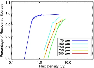
To quantify the degree of completeness of the extracted source lists, we carried out an extensive set of artificial source exper-iments by injecting simulated sources into real Hi-GAL maps. Given the very time-consuming nature of these experiments, we chose to carry them out for each band, but only for a subset of the entire range of longitudes that is the subject of the present release. We visually selected one from every two to three tiles, depending on the variation of the emission seen in the maps as a function of Galactic longitude. We used a similar methodology as in Sect.4.2to determine the optimal extraction threshold, but this time we used only one detection threshold and an adaptive grid of trial fluxes for the synthetic sources.
For each band of this subsample, we injected 1000 sources modelled as elliptical Gaussians of constant integrated flux, with sizes and axis ratios equal to the majority of the compact sources determined from the initially extracted list (see Figs.18and19). In this way, we were able to test the ability to recover a statis-tically comparable population of sources from the same map. The sources were randomly spread on the map, with the only constraint being to avoid overlap with the positions of the real sources.
The simulated data were processed with C
u
TEx
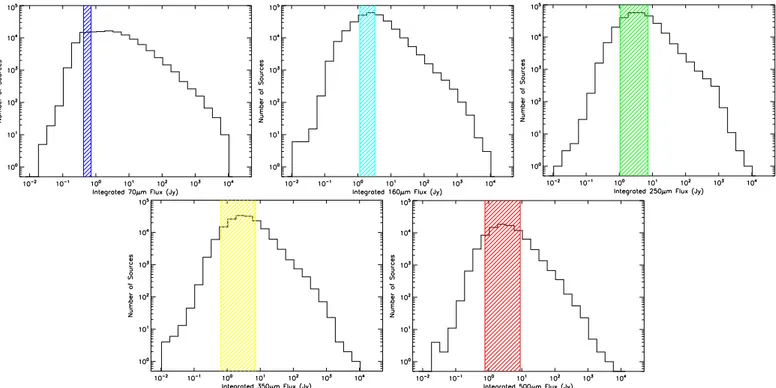
, adopting the same setup of parameters as used for the initial list, and the outputs were compared with the truth table of the injected sources. To estimate the errors, we iterated the experiment ten times and determined the variation in the fraction of recovered sources. The same process was iterated for different values of integrated flux until we recovered 90% of the sources (with a tolerance of 1%). An example of the recovery fraction as a func-tion of the integrated flux density of the injected sources is given in Fig.8.In Fig. 9 we show the estimated completeness limit as a function of Galactic longitude. The limits for the PACS 70 µm and 160 µm bands are quite regular along the whole range of
Fig. 9.Ninety percent completeness limits in flux density for a popula-tion of sources with the same distribupopula-tion of sizes as the one extracted by C
u
TEx
as a function of Galactic longitude. The significant increase in the completeness limit in the inner Galaxy and especially close to the Galactic centre is due to the brighter background emission in such regions.longitude. However, while the completeness in the 70 µm band is almost constant, at 160 µm it is higher for |`| ≤ 40◦. This
behaviour is more significant in the SPIRE wavebands and in-creases while moving toward the Galactic centre. It is explained by the overall brighter emission at lower longitudes, making the detection of fainter objects a harder task, even with the strong damping induced by C
u
TEx
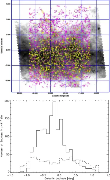
.The completeness limits reported in Fig.9should be seen as conservative because they are determined by spreading the syn-thetic sources randomly over each entire tile. However, the dif-fuse background is highly non-uniform in each tile, but it is dom-inated by the strong GP emission with a maximum in the central horizontal section of each map, and then decreasing toward the north and south Galactic directions. A typical example is offered in Fig.10, where the upper panel shows the 250 µm image of the tile centred at ` = 41◦. Superimposed are the extracted 250 µm compact sources with integrated fluxes above (yellow crosses) and below (magenta crosses) the flux completeness limit appro-priate for the Galactic longitude at that band (3 Jy, from Fig.9). This is also shown in the lower panel of Fig.10, where the lat-itude distribution of the two groups of sources is also reported with full and dashed lines for sources above and below the con-fusion limit.
The two groups of sources have a very different spatial distri-bution, with sources brighter than the completeness limit mostly concentrated at –0◦.6 ≤ b ≤ 0◦.2, while the fainter sources are uniformly distributed and mostly found toward the map areas where the diffuse emission is relatively less intense. The dashed line in the lower panel histogram is flat because fainter sources are better detected in lower surface-brightness regions (above and below the plane) than in the central band of the plane.
In subsequent releases of the Hi-GAL photometric cata-logues we will provide more precise estimates of the catalogue completeness limits specific to different background conditions.
4.5. Deblending
CuTEx is designed to fit a Gaussian function to each posi-tion that shows an enhancement of the second derivative with
Fig. 10.Upper panel: 250 µm image of the Hi-GAL tile at `= 41◦
. Su-perimposed are the sources detected with C
u
TEx
. The yellow crosses indicate the sources with fluxes above the completeness limit, while the magenta crosses indicate the sources with fluxes below the com-pleteness limit. Lower panel: histograms of latitude distributions for 250 µm sources, above (full line) and below (dashed line) the complete-ness limit.respect to its nearby environment. While the flux estimate re-lies on the performance of the fitting engine as well as on the fidelity of the Gaussian model fit to the real source profiles, it is clearly important to quantify the ability of the photometric al-gorithm to separate individual sources when they are very close to each other. To quantify the deblending performance of the al-gorithm, we generated simulations with 2000 sources randomly distributed in a region whose size represents the typical foot-print of the Hi-GAL maps. For every set of positions we pro-duced two different sets of simulated populations. In the first case, we injected sources with sizes of the order of the beam size. In the second case we simulated a population of extended sources modelled as elliptical Gaussians with the FWHM of one of the two axes drawn from a uniform distribution between 1 and 2.5 times the beam size. The other axis was determined by assuming an axis ratio randomly drawn from a uniform distribu-tion between 0.5 and 1.5 times the beam size. The input sources were randomly oriented. We computed several simulations with
0 10 20 30 40 50 60 Separation (arcsec) 0.0 0.2 0.4 0.6 0.8 1.0 1.2
Fraction of Blended Sources
Fig. 11.Curves represent the fraction of blended sources that C
u
TEx
is not able to deblend as a function of source separation for a set of synthetic sources described in the text; simulations in this case are made for the 250 µm images. The full and dashed lines are the results for simulations with extended and point-like sources, respectively. Vertical lines represent the size of the beam (dashed), and 75% the size of the beam (dotted).
different positions and increasing source densities to estimate the deblending performance for cases of both lesser and greater clustering.
We processed the simulations with CuTEx and determined its ability to correctly identify individual sources as a function of the source pair separation. Because of the large number of sources and their relatively high densities, there are several thou-sand source pairs in each simulation that can be tested for the effectiveness of our deblending algorithm. We plot in Fig.11the fraction of source pairs that are not resolved into their separated components as a function of their relative separation for simu-lations of the 250 µm data (where the maps have a pixel size of 600). Similar curves are found for the other wavelengths. The er-ror bars represent the amplitude of such a fraction found in the whole set of simulations. The full line refers to the population of extended sources, while the dashed line indicates the results for the sample of point sources. The vertical dashed line traces the size of the beam, while the dotted line traces 0.75 times the beam.
Figure11shows that CuTEx is able to deblend sources quite effectively. Point-like sources are resolved perfectly up to dis-tances that are ∼0.8 times the beam, while extended sources are properly deblended and identified for distances larger than ∼1.25 times the beam. For the extended source case, half of the source pairs that are separated by a single beam size are deblended. Clearly, the Gaussian fit for a blended source pair will result in a larger size estimate than the case where the two components are resolved by the detection algorithm.
4.6. Photometric corrections to integrated fluxes
The flux of the source candidates is derived from the parameters of the 2D-Gaussian fit found with C
u
TEx
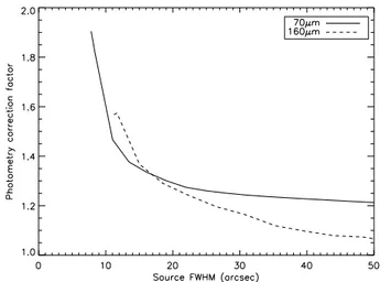
. While a 2D Gaussian is a good and acceptable approximation for the PSF of SPIRE (SPIRE Instrument Team & Consortium 2014), the same is not true for PACS because of the observing setup adopted for the Hi-GAL survey. The on-board coaddition (in groups of eight frames at 70 µm and four frames at 160 µm) while scanningFig. 12.Correction factors to be applied to C
u
TEx
photometry as afunction of the source FWHM. The values are only applicable for im-ages obtained similarly to Hi-GAL.
the satellite, results in substantially elongated beams (see Sect.2 above) that show significant departures from a circularly sym-metric morphology. Part of this asymmetry is mitigated by the coaddition of scans in orthogonal directions, but significant de-partures from an ideal Gaussian symmetry persist. It is then nec-essary to estimate correction factors to be applied to the extracted C
u
TEx
photometry to account for the (incorrect) assumption of Gaussian source brightness profiles assumed by Cu
TEx
.We adopted an empirical approach to estimate the correc-tions to the C
u
TEx
photometry of PACS images. This was done by performing Cu
TEx
photometry, using the same settings as used for the Hi-GAL catalogues, on an image of a primary Herschelphotometric calibrator – α Bootis. α Bootis was ob-served during OD 269 in the same conditions as the Hi-GAL observations (i.e. with two mutually orthogonal scan maps in parallel mode with a scanning speed of 6000/s). The α Bootis images present a nice and clean point-like object with no de-tectable diffuse emission background (ideal photometry condi-tions compared to Hi-GAL). To extend the photometric correc-tion factors to the more general case of compact but resolved sources, we convolved the images of α Bootis with a 2D-circular Gaussian kernel of increasing size while normalizing integrated flux (i.e. flux conserving). The convolving kernels span the inter-val [0.0, 5.0] × θ0in steps of 0.5θ0, where θ0is the FWHMde-rived from the unconvolved α Bootis profile. C
u
TEx
integrated fluxes for the entire set of simulations were then compared with the expected values in the PACS bands as derived from theo-retical models (Müller et al. 2014). After applying a colour cor-rection estimated followingPezzuto et al.(2012), the fluxes of α Bootis used for the comparison are 15.434 and 2.891 Jy at 70 and 160 µm, respectively. Figure 12 reports the correction factors as estimated from the above analysis as a function of the FWHM of the compact source considered. The correction factors decrease rapidly from point-like to minimally resolved sources. With larger sources, the decrease in the correction factor is a weaker function of source size. Beam asymmetries, however, are clearly persistent and detectable even for relatively extended sources.The integrated fluxes for each source in the 70 and 160 µm catalogues were corrected using the curves in Fig. 12 and the sources’ circularised size (see Sect. 5.3). Both the uncor-rected and the coruncor-rected integrated fluxes are reported in the columns FINT and FINT_UNCORR of the source catalogues