Inflation persistence: Implications for a design of monetary
policy in a small open economy subject to external shocks
Karlygash Kuralbayeva
CEIS Tor Vergata - Research Paper Series, Vol.
32, No.95, March 2007
This paper can be downloaded without charge from the Social Science Research Network Electronic Paper Collection:
http://papers.ssrn.com/paper.taf?abstract_id=962665
CEIS Tor Vergata
R
ESEARCH
P
APER
S
ERIES
In‡ation persistence: Implications for a design of monetary
policy in a small open economy subject to external shocks
Karlygash Kuralbayeva
Lincoln College, University of Oxford
August 15, 2006
Abstract
We analyze implications of in‡ation persistence for business cycle dynamics following terms of trade and risk-premium shocks in a small open economy, under …xed and ‡exible exchange rate regimes. We show that the country’s adjustment paths are slow and cyclical if there is a signi…cant backward-looking element in the in‡ation dynamics and the exchange rate is …xed. We also show that such cyclical adjustment paths are moderated if there is a high proportion of forward-looking price setters. In contrast, with an independent monetary policy, ‡exible exchange rate allows to escape severe cycles, supporting the conventional wisdom about the insulation role of ‡exible exchange rates.
JEL Classi…cations: E32, F40, F41
Keywords: in‡ation inertia, monetary policy, exchange rates, persistence, Phillips curve, small open economy
1
Introduction
The debate regarding the choice of an exchange rate regime is very old, and yet it remains to be controversial. The theoretical literature provides broad guidance on the choice of exchange rate. Much of the modern analysis of choosing an exchange rate regime goes back to the works of Friedman (1953), Mundell (1963) and Fleming (1962). Friedman (1953) made the modern case for a ‡exible exchange rate: a ‡exible exchange rate is desirable in the face of real country-speci…c shocks that require adjustment in relative prices between countries, because nominal prices are highly in‡exible. However, if prices are ‡exible, the choice of exchange rate is irrelevant as adjustment in relative prices can happen either via changes in the nominal exchange rate or prices.
Address: Lincoln College, Turl Street, OX1 3DR, Oxford, UK, email: [email protected] I am indebted to David Vines for helpful comments and guidance. I am particularly grateful to Florin Bilbiie for many helpful and detailed comments at di¤erent stages. I also bene…ted from comments from Gianluca Benigno, Fabio Ghironi, Tatiana Kirsanova and Richard Mash. The paper has been presented at the Gorman Workshop, University of Oxford and XV International "Tor Vergata" conference on Banking and Finance, University of Rome "Tor Vergata". The paper has been awarded as the best young economist paper presented at the "Tor Vergata" conference. All errors are mine.
Friedman’s analysis has been extended by Mundell (1963) and Fleming (1962) to a world of capital mobility1. Following their work, one of an important considerations in the choosing
of an exchange rate regime have become the nature and source of the shocks to the economy and the degree of capital mobility. In general, a …xed exchange rate in an open economy with capital mobility is preferable if the shocks bu¤eting the economy are predominantly monetary, such as changes in the demand for money. A ‡exible exchange rate is preferable if shocks are predominantly real, such as changes in technology or tastes2.
The emergence of an important strand of macroeconomics, called New Open Economy Macro-economics (NOEM)3, enabled analysis of the design of monetary policy and the choice of ex-change rate in an open economy within stochastic, sticky-price general equilibrium optimizing models. General equilibrium sticky-models, based on utility maximization, allow to examine welfare consequences of alternative monetary rules. Now there is a lengthy literature that stud-ies the performance of monetary rules (optimal or not) in open economstud-ies4. From traditional NOEM models the general consensus has emerged that countries should allow their exchange rates to ‡oat freely and use monetary policy to target some measure of in‡ation.
Despite the insulating role of ‡exible exchange rates in open-economies in the face of real shocks, greater …xity of exchange rate may be justi…ed on many grounds. For example, in many small open economies exports, imports and international capital ‡ows represent a large share of their economies, so large variations in the exchange rate can cause very large variations in the real economy. Another argument in favor of greater …xity of the exchange rate is the liabil-ity dollarization – phenomenon, which is characterized by external net liabilities denominated in dollars and revenues generated in local currency. In this case, a sharp real exchange rate depreciation causes a decline in the net worth of corporations and individuals, leading to a sharp decline in lending and hence economic contraction. This situation can be exacerbated in the presence of …nancial imperfections, which can arise from informational asymmetries or institutional shortcomings, and which imply that borrowers face constraints. In this case, the contractionary e¤ect of an exchange rate depreciation works through the negative …nancial ac-celerator channel, which links the condition of the borrower’s balance sheets with the terms of credit. A sharp depreciation, which reduces earnings of …rms and deteriorates their balance sheets, decreases …rms’capacities to borrow and invest. This discussion suggests that …nancial vulnerability is a su¢ cient reason for abandoning a ‡oating exchange rate in favor of a more …xed rate. However, a number of papers that incorporate the …nancial accelerator mechanism in general equilibrium setting with nominal rigidities (e.g., Céspedes et al., (2000), Gertler et
1
See Bordo (2003) for survey of the issues relating to exchange rate regime choice in historical perspective.
2When shocks come from the money market, a country bene…ts from a …xed-rate regime. The shock would
be absorbed through purchases and sales of foreign exchange by the monetary authority, which would a¤ect the money supply, maintain a …xed exchange rate, and keep real output una¤ected. With sticky wages and prices, countries that are subject to real shocks are better o¤ with a ‡exible exchange rate. In the face of negative real shocks, a depreciation of the exchange rate would reduce the price of tradable goods and ensure expenditure switching from more expensive foreign goods to relatively cheaper domestically produced goods, and thus o¤set the negative e¤ect of the shock.
3Literature survey, see Lane (2001) 4
Aoki (2001), Galí and Monacelli (2002), Ghironi and Rebucci (2001), Parrado and Velasco (2001), among others
al. (2003), Devereux et al. (2004)) claim that the presence of such …nancial frictions amplify the business cycle, but do not alter conventional wisdom that ‡exible exchange rate are less contractionary than …xed rates and ‡exible exchange rates are optimal from a welfare point of view.
One feature that characterizes most of the models discussed above is the entirely forward-looking nature of price setting behavior5. The models of these papers specify nominal rigidities by assuming a time-contingent staggered Calvo (1983) price setting mechanism that generates a standard forward-looking New Keynesian Phillips Curve (NKPC)6. The forward-looking nature of the NKPC, in turn, implies a great deal of ‡exibility for the dynamics of in‡ation. This, however, is in contrast with empirical evidence, which suggests that in‡ation is highly persistent7.
In this paper we develop a dynamic general equilibrium small open-economy model, where in‡ation persistence is incorporated via introduction of rule-of-thumb price setting. We use this model to study the e¤ects of such backward-looking behavior on dynamic adjustment in response to the shocks. The paper aims to explore the implications of in‡ation inertia for business cycle dynamics in the face of terms of trade and risk-premium shocks. In our framework, nominal and real exchange rates play a central role in the adjustment process when prices are sticky. Therefore, our discussion focuses on the question of the insulating properties of alternative exchange rate regimes. We study two commonly-used monetary policies: a …xed exchange rate (when the monetary authority stabilizes the nominal exchange rate) and a ‡exible exchange rate (when the central bank stabilizes in‡ation).
Our paper is related to two strands of the literature. The …rst is one that studies performance of simple monetary rules (whether optimal or not) in a dynamic New Keynesian framework, brie‡y discussed above. The second focuses on empirical evidence of in‡ation persistence, its determinants and implications for a design of monetary policy.
As we have noted earlier, most of the papers within the literature on the performance of monetary rules in open economies focus on a standard forward-looking Phillips curve that ex-hibits no intrinsic persistence. However, there are many more models that incorporate in‡ation persistence into stochastic general equilibrium settings with nominal rigidities to study di¤erent issues (e.g., Christiano et al. (2001), Leitemo (2002), Benigno and Thoenissen (2003), Smets and Wouters (2002)). Our paper is probably closest to Leitemo (2002), who analyzes the insulating role of alternative monetary policy regimes for di¤erent degrees of in‡ation persistence. Contrary to our paper, Leitemo illustrates the signi…cance of di¤erent monetary policy regimes, both for a reduction of volatility in key macro variables in the face of shocks and for welfare (we, however, do not look at welfare). In particular, Leitemo …nds that social loss under di¤erent monetary regimes is lower when there is less in‡ation persistence, and perhaps the most important …nding is that the currency-board arrangement (as well as the exchange-rate targeting regime) achieves the greatest improvement in terms of a social loss as in‡ation becomes more forward-looking.
5
Some research from the late 1990s has disregarded the forward-looking term in the Philips curve and focused on entirely backward-looking speci…cation of the curve (see for example Svensson (1997) and Rudebusch and Svensson (1999)). However this research is not set in a micro-founded framework.
6
See the analysis and discussion related to the New Keynesian model in Clarida et al. (1999), who also provide references to the extensive literature related to this model.
7
However, it is important to note that, his model is a one-sector model, which embodies some mi-crofoundations and adheres to non-structural arguments in representing persistence in in‡ation and output.
Our paper is also related to a lengthy literature that analyzes implications of in‡ation inertia for a design of monetary policy8. Within this strand of the literature there is a large body of research that investigates the implications of in‡ation persistence in the context of a monetary union. Benigno and Lopez-Salido (2002) analyze di¤erent in‡ation targeting policies under the presence of heterogeneity in in‡ation dynamics across euro area countries. By using, a micro-founded New Keynesian framework, they evaluate the welfare implications of di¤erent in‡ation targeting policies. A vital complement to work by Benigno and Lopez-Salido (2002) of investigation of optimal policies is an analysis of the stability of models under particular policy regimes, which have been thoroughly examined in a monetary union by Kirsanova et al. (2006). They show how members of the monetary union can be vulnerable to cyclical instability and show how the active use of …scal policy can be used to mitigate or avoid this problem. Kirsanova et al. (2006a) also demonstrate that a higher proportion of forward-looking price setters moderate destabilizing e¤ects following asymmetric shocks in the monetary union. These results agree with Westaway (2003) and Allsopp and Vines (2006), who also point out that a destabilizing tendency in the monetary union following shocks can be aggravated by more signi…cant backward-looking element in in‡ation behavior. Analogous to their work, our paper aims to analyze dynamic adjustment in the face of external shocks in a small open economy, where backward-looking behavior is introduced. In‡ation in the country is governed by a Phillips curve, that may be either backward-looking (accelerationist) or forward-looking (New Keynesian). We deliberately focus on these two limiting speci…cations of the Phillips curve to examine how backward-looking behavior changes the propagation of the shocks to the economy compared with a forward-looking speci…cation, which has been extensively studied in the literature. We perform our analysis under two exchange rate regimes, a …xed rate and a ‡exible exchange rate, which allows us to discuss whether a small open economy will bene…t from a ‡exible exchange rate in the presence of a substantial fraction of backward-looking price setters.
The reminder of the paper is structured as follows. Section 2 describes the model and de…nes a competitive equilibrium for the economy. Section 3 discusses calibration of the model. We discuss the simulation results in section 4. Section 5 concludes.
2
Model of a Small Open Economy
We consider a two sector dynamic stochastic general equilibrium model with nominal rigidities. The domestic economy is open and small and comprises three sectors: traded, non-traded goods, and the oil sector. We assume that oil production requires no domestic factor inputs, and all of its production is exported. The exogenous price of oil is subject to stochastic shocks. Our model assumes ‡exible price traded goods, traded in competitive markets, and a continuum of monopolistically produced non-traded goods. We assume Calvo-type price stickiness in the
8
A general overview of results for optimal policy in the presence of backward-looking settings is provided in Levin and Moessner (2005).
non-traded sector. While most of the papers that use the small open economy framework em-body nominal inertia in terms of the form of Calvo contracts, we also allow for some additional in‡ation inertia, using a rule-of-thumb price setting mechanism outlined in Steinsson (2003). Domestic households consume both non-traded and traded goods. Traded goods could also be invested and imported from the rest of the world. Non-traded goods are also used to meet capital installation costs, which are a composite of both non-traded and traded goods in the same mix as the household’s consumption basket. Households own production …rms, supply labor and accumulate capital that they rent to production …rms. As the owners of the …rms producing non-traded goods, households also receive the income corresponding to the monop-olistic rents generated by these …rms. Non-traded goods …rms produce di¤erentiated varieties of non-traded goods. We consider two alternative monetary policy regimes: ‡exible and …xed exchange rate regimes. In both cases the monetary authority uses the nominal interest rate as a policy instrument and monetary policy is modeled through an interest rate rule.
2.1 Consumers
Consider a small open economy with non-traded goods, traded goods and oil. The economy is inhabited by a continuum of households with mass 1. The representative consumer has preferences given by:
U = E0 1 X t=0 tu(C t; Ht) (2.1)
where Ctis a composite consumption index and Htis the labor supply. We assume the following
functional form of utility function u:
u = C 1 t 1 H1+ 1 +
Composite consumption is a constant-elasticity-of-substitution (CES) function of traded goods and non-traded goods, with
Ct= [a
1
CN;t( 1)= + (1 a)1CT;t( 1)= ] =(1 ); > 0; : (2.2) with CN;t and CT;t being indexes of consumption of non-traded and traded goods respectively.
Under such speci…cation of the composite consumption function, the parameter measures the (inverse) intertemporal elasticity of substitution and the parameter is the intratemporal elasticity of substitution between non-traded and traded goods. The implied consumer price index is then
Pt= [aPN;t1 + (1 a)PT;t1 ]
1 1
where PN;tis the price index of the composite di¤erentiated non-traded good, PT;tis the price of
‡exible-price traded good, expressed in national currency, and Pt is the consumer price index.9
9
The price index Ptis the minimum expenditure required to purchase one unit of aggregate consumption good
Indexes of consumption of non-traded goods, in turn, is given by CES aggregators of the quan-tities consumed of each variety, with elasticity of substitution across di¤erent categories equal to : CN t= ( Z 1 0 CN;t(j) 1 dj) 1; with > 1 (2.3)
where CN;t(j) is consumption of variety j by the representative household. When tends to
in…nity all varieties are perfect substitutes for each other. The price of variety j is denoted PN;t(j), and the price of a consumption basket of non-traded goods PN;t is de…ned as a CES
index10 with elasticity 1= :
PN;t= (
Z 1
0
PN;t(j)1 dj)1=(1 ) (2.4)
The optimal allocation of any given expenditure on non-traded goods yields the total demand for variety j 2 [0; 1] :
CN;t(j) = (
PN;t(j)
PN;t
) CN;t;
Households may borrow and lend in the form of non state-contingent bonds that are denom-inated in units of the traded goods. We assume that the borrowing rate iFt ; charged on foreign debt depends on an exogenous world interest rate, i ; and exogenous term t that capture external shocks to the borrowing rate:
(1 + iFt ) = (1 + i )(1 + t) (2.5) The exogenous part of the foreign rate t follows a partial adjustment process:
log( t) = (1 ) log + log( t 1) + "t; E("t) = 0; var("t) = 2 (2.6) Observe that in this paper we do not endogenize the interest rate, and do not use other methods (…nitely-lived households, transactions costs in foreign assets, endogenous discount factor11) to rule out the nonstationary behavior of consumption and the current account. The nonstationary behavior of variables implies that unconditional variances do not exist, which poses problems for business cycle analysis. However, we are not interested in such analysis. In addition, the non-endogenized speci…cation of foreign interest rate allows us to compare our results with the real business cycle (RBC) analogue of the model of this paper, discussed in Kuralbayeva and Vines (2006), which also assumes an interest rate speci…cation similar to (2.5). Households can also obtain loans from domestic capital markets, with Bt the stock of domestic
currency debt.
Households own …rms that produce two goods: traded and non-traded goods in the economy. Households accumulate capital and rent it out to the goods producing …rms. Capital stocks in non-traded and traded sectors are assumed to evolve according to the following:
1 0
This price index is the minimum expenditure required to buy one unit of aggregate consumption non-traded good CN;t:For the derivation see, for example, Corsetti and Pesenti (2005).
1 1
KN;t+1= IN;t+ (1 )KN;t; (2.7)
KT;t+1= IT;t+ (1 )KT;t; (2.8)
where investment in both sectors is traded good. Installation of capital in both sectors requires adjustment costs, which represent a basket of goods composed of non-traded goods and traded goods in the same mix as the household’s consumption basket. We de…ne capital adjustment costs as: i;t( Ii;t Ki;t )Ki;t = I 2 ( Ii;t Ki;t )2Ki;t; where i = N; T; so 0 > 0; and 00> 0:
The household’s budget constraint in nominal terms is:
PtCt+ Pt( N tKN t+ T tKT t) + PT t(IN t+ IT t) = WtHt+ StDt+1 (1 + iFt )StDt+ Bt+1 (1 + it)Bt+ RN tKN t+ RT tKT t+ PT tOt+ Z 1 0 N t(j)dj (2.9) where Wt is the wage rate; RN t and RT t are the nominal rates of return for households in
the non-traded and traded sectors respectively; Dt is the outstanding amount of foreign debt,
denominated in foreign currency, Bt is the stock of domestic debt, denominated in domestic
currency, and St is the nominal exchange rate expressed as units of domestic currency needed
for one unit of foreign currency. The household owns KN;t and KT;t units of capital in the
non-traded and traded sectors, makes additional investments in both sectors of IN;t and IT;t,
consumes Ct and supplies Ht units of labor, and receives pro…ts from the …rms producing the
non-traded goods,R01 N t(j)dj:
The household optimum is characterized by the following equations:
Wt= Ht PtCt (2.10) 1 = Et[ CtPt Ct+1Pt+1 (1 + it+1)] (2.11) 1 = Et[ CtPt Ct+1Pt+1 St+1 St (1 + iFt+1)] (2.12) qNt = Et CtPt Ct+1Pt+1fRN t+1 + Pt+1( 0N;t+1 IN t+1 KN t+1 N;t+1 ) + qNt+1(1 )g (2.13) qtN = PT t+ Pt `N;t (2.14)
qTt = Et CtPt Ct+1Pt+1fRT;t+1 + Pt+1( `T;t+1 IT;t+1 KT;t+1 T;t+1 ) + qt+1T (1 )g (2.15) qtT = PT t+ Pt 0T;t (2.16)
along with the capital accumulation, (2.7)-(2.8), and budget constraint, (2.9), equations. Equation (2.10) equates the marginal disutility of the labor e¤ort to the utility value of the wage rate, and de…nes the households labor supply curve. Equation (2.11) is a Euler equation that determines intertemporal allocation: it equates the intertemporal marginal rate of sub-stitution in consumption to the real rate of return on domestic bonds. Equation (2.13) is the counterpart of equation (2.12) for foreign bonds. Equation (2.13) is the pricing condition for physical capital in the non-traded sector. It equates the revenue from selling one unit of capital today (qtN), to the discounted value of renting the unit of capital for one period, and then selling it, RN;t+1+ qt+1N ; net of depreciation and adjustment costs12. Equation (2.14) relates the cost
of producing a unit of capital in the non-traded sector to the shadow price of installed capital, or Tobin’s Q, qtN: Equations (2.15), and (2.16) are the traded sector counterparts of (2.13) and (2.14). Equation (2.11) in conjunction with (2.12) yields the uncovered interest parity condition (UIP): EtfCt+1 Pt Pt+1 [(1 + it+1) (1 + iFt+1) St+1 St ]g = 0 (2.17) Given a decision on consumption Ct the household allocates optimally the expenditure on
CN;t and CT;t by minimizing the total expenditure PtCt under the constraint (2.2), so demands
for non-traded and traded goods are:
CN t= a( PN;t Pt ) Ct (2.18) CT t= (1 a)( PM;t Pt ) Ct (2.19) 2.2 Production by Firms
We assume a continuum of monopolistically competitive …rms of measure unity in the non-traded sector, each producing output with the production function:
YN;t(j) = ANKN;t(j) HN;t(j)1 (2.20)
where AN is a productivity parameter, which is the same across the …rms in the non-traded
sec-tor. Firms in the traded sector operate under perfect competition with the production function given by:
YT;t(j) = ATKT;t(j) HT;t(j)1 (2.21)
1 2
Adjustments are costs stemming from decreasing the capital stock. The installation function N tKN t
as a function of IN t shifts upwards as KN t decreases, which is represented by @=@KN t+1( N t+1KN t+1) = 0
where AT is a productivity parameter, and is also the same across the …rms in the traded sector.
There are also a mass of one of …rms producing traded goods. We assume all …rms rent capital and labor in perfectly competitive factor markets. Cost minimization implies equations:
Wt= M CN;t(1 ) YN;t HN;t (2.22) RN;t= M CN;t YN;t KN;t (2.23) Wt= PT;t(1 ) YT;t HT;t (2.24) RT;t= PT;t YT;t KT;t (2.25) where YN;t = ANKN;t HN;t1 and YT;t = ATKT;t HT;t1 are aggregate supply functions of
non-traded and traded goods13. Demand for labor and capital in the non-traded goods sector
is described by equations (2.22)-(2.23), where M CN;t represents the (nominal) marginal costs
in that sector. It is noteworthy that the marginal costs in the non-traded sector are identical across …rms as long as their production functions exhibit constant returns to scale and prices of inputs are fully ‡exible in perfectly competitive markets. Producers of the traded goods are price-takers, so that equations (2.24)-(2.25) describe the demand for labor and capital inputs in the traded sector, with PT;t representing the unit cost of production.
2.3 Price setting in the non-traded sector
In order to describe the price setting decisions we split …rms into two groups according to their pricing behavior, following Steinsson (2003). In each period, each …rm changes its price with probability 1 N, and otherwise, with probability N; its price will rise at the steady state
rate of in‡ation N;t= PN;t=PN;t 1. Among those …rms which reset their price, a proportion of
1 ! are forward-looking and set prices optimally, while a fraction ! are backward-looking and set their prices according to a rule of thumb.
Forward-looking …rms are pro…t-maximizing and reset prices (PN;tF ) optimally, which in terms of log-deviations from the steady state (see Technical appendix) implies:
b pFN;t=mccN;t+ Et 1 X i=1 ( N )i[mccN;t+i mccN;t+i 1] + Et 1 X i=1 ( N )i N;t+i (2.26)
where N;t is in‡ation in the non-traded sector and mccN;t stands for the deviation of real
marginal costs from its steady state. As discussed in Christiano et al. (2001), relation (2.26) shows several important features of the behavior of the forward-looking …rms. When …rms expect real marginal costs to be higher in the future and/or expect future increases in the price
1 3
With respect to aggregation in the non-traded sector, in the appendix we show that the non-traded market equilibrium equation has an additional term that deals with the distribution of prices in the non-traded sector. However, as shown in the appendix (see also Yun (1996), Erceg et. al. (2000) and Christiano et. al. (2001)), this term does not appear in the log-linear approximation of the resource constraint in the non-traded sector.
level, then the …rms setpbFN;t higher thanmccN;t: Christiano et al. (2001) describe this behavior
as ‘front loading’. Firms understand that they might not be allowed to change their price when higher real marginal costs or higher prices materialize. So, anticipating this, forward-looking …rms set prices to maximize their current and future pro…ts, taking into account the future evolution of real marginal costs and prices. Further, for derivation of the Phillips curve below, it is convenient to re-write relation (2.26) as:
b
pFN;t= (1 N)mccN;t+ NpbFN;t+1+ N N;t+1 (2.27)
Backward-looking …rms set their prices according to the following rule14:
PN;tB = PN;t 1r N;t 1(
YN;t 1
YN;t 1n )
# (2.28)
where N;t 1= PN;t 1=PN;t 2 is the past period growth rate of prices in the non-traded sector,
YN;t 1=YN;t 1n is output relative to the ‡exible-price equilibrium, PN;t 1r is an index of prices set
at date t 1, given in terms of log-deviations from the steady state (see Appendix) by: b
prN;t 1= (1 !)pbFN;t 1+ !pbNN;t 1 (2.29) The rule of thumb (2.28) shows that backward-looking …rms set their prices equal to the average of the newly set prices in the previous period updated by the previous period in‡ation rate of the non-traded goods price level and by the deviation of the non-traded goods output relative to the ‡exible price equilibrium non-traded output. This assumption, as discussed in Galí and Gertler (1999) has the following appealing properties: …rst, the rule of thumb behavior converges to the optimal behavior over time; and second, PN;tB depends only on information up to the period t 1, but implicitly incorporates past expectations about the future, since the price index PN;t 1r is partly determined by forward-looking price setters.
For the whole non-traded sector, the price index in the non-traded sector is given by:
PN;t= [(1 N)(1 !)(PN;tF )1 + (1 N)!(PN;tB )1 + N( NPN;t 1)1 ]
1
1 (2.30)
Following Steinsson (2003), we can derive the following Phillips curve for the non-traded sector, written in terms of log-deviations from the steady state15:
N;t= f Et N;t+1+ b N;t 1+ 1byN;t 1+ 2byN;t+ mcmccN;t (2.31)
1 4There is no consensus on a way of introducing in‡ation persistence. In the micro-founded way there are two
main mechanisms. First is a rule-of-thumb price-setting behaviour that we follow in this paper (see also Kirsanova et. al. (2006)). The second mechanism is a backward-looking price indexation (Christiano et. al. (2001), Smets and Wouters (2002), Woodford (2003)). Each period only a fraction of …rms re-optimize their prices, while the remaining …rms index their prices to a fraction of the lagged in‡ation rate. As an alternative to micro-founded mechanisms above, in‡ation intertia can be modeled on the basis of adaptive expectations as in Roberts (1997), on the basis of sticky information as in Mankiw and Reis (2001), or as a signal extraction problem in Erceg and Levin (2001).
1 5
The derivation is identical to one in Steinsson (2003) and Kirsanova et. al. (2006), amended by the introduc-tion of the real marginal costs and by accounting for the non-traded sector. A detailed derivaintroduc-tion is given in the technical appendix.
where the coe¢ cients are: f = N N + !(1 + N N) ; b= ! N + !(1 + N N) ; 1 = !#(1 N) N + !(1 + N N) ; 2= N !#(1 N) N + !(1 + N N) ; mc= (1 N)(1 !)(1 N) N+ !(1 + N N) :
and where ybN;t is the output gap in the non-traded sector, de…ned as the deviation from the
‡exible price output of the non-traded sector (YN;tn ); and mcN;t are real marginal costs in the
non-traded sector.
All coe¢ cients are explicit functions of three model parameters: N which measures the
degree of price stickiness in the non-traded sector; ! which measures the degree of ‘backwardness’ in price setting, and the discount factor : Coe¢ cients on the output gaps, 1and 2; also depend
on the elasticity #: In this model, the degree of in‡ation inertia can be measured by the fraction of backward-looking …rms, as a larger fraction of backward-looking …rms implies a higher value of the coe¢ cient of the lagged in‡ation, b: As one would anticipate, a rise in ! leads to a
fall in the coe¢ cients of current variables, 2 and mc, and to a rise in the coe¢ cient of the
predetermined variable, 1: Moreover, a higher degree of backwardness in the model implies a
lower weight on the currently expected future in‡ation, f: This is because only forward-looking
…rms react immediately to changes in current market conditions.
Note that when ! = 0 the Phillips curve collapses to the standard forward-looking speci…-cation:
N;t=
(1 N)(1 N)
N c
mcN;t+ Et N;t+1= NmccN;t+ Et N;t+1 (2.32)
When ! = 1 the Phillips curve takes the speci…cation:
N;t= N 1 + N Et N;t+1+ 1 1 + N N;t 1 1 N 1 + N [ N#ybN;t #byN;t 1] (2.33)
As noted in Steinsson (2003), (2.33) has a unique bounded solution:
t= t 1+ (1 N)#ybN;t 1 (2.34)
which is a form of the accelerationist Phillips curve and has no forward-looking component.
2.4 Local Currency Pricing
We assume that the price of the traded good is ‡exible and determined by the law of one price, so:
PT;t= StPT;t
where PT;tis the foreign currency price of the traded good, and St is the nominal exchange rate.
The economy is small also in the respect that the economy’s export share is negligible in the foreign aggregate price index, implying that the foreign price of traded goods is equal to the
foreign aggregate price level, and we assume that it is equal to unity, so PT;t = Pt = 1, and PT;t= St:
De…ning the real exchange rate as, et = StPt=Pt; so the real exchange rate depreciates
(appreciates) when et rises (decreases). The rate of change of the real exchange rate is given as:
et
et 1
= 1 + t 1 + t
(2.35) and the nominal exchange rate depreciation in period t is given by:
1 + t=
St
St 1
(2.36)
2.5 Monetary policy
We assume that the monetary authority uses the nominal interest rate as the policy instrument. We consider two alternative monetary policy regimes: ‡exible and …xed exchange rate regimes. In the …rst, the ‡exible exchange rate regime monetary policy is characterized as a Taylor rule:
log(1 + it 1 + i) = Y log( YN t YN;tn ) + log( 1 + N;t 1 + N ) (2.37)
where N is the target for the annual in‡ation in the non-traded sector, i is the stationary value
of the interest rate, and YN;t=YN;tn is output of the non-traded sector relative to its ‡exible-price
equilibrium. Log-linearization of the feedback rule yields:
bit= YybN;t+ t (2.38)
where Y > 1; and > 0 are the reaction coe¢ cients on non-traded goods in‡ation andybN;t is
the output gap in the non-traded sector.
Alternatively, monetary policy is characterized by the following interest rate rule that delivers a …xed exchange rate:
1 + it= (1 + iFt )(
St
S)
!S (2.39)
where !S > 0; and St = S 8t: Under this rule, the monetary authority pegs the nominal
exchange rate at a target level S in all periods by varying the nominal interest rate in reaction to movements in the foreign interest rate and deviations of the nominal exchange rate from the target16.
2.6 Equilibrium
The equilibrium of the economy is a sequence of prices fÞtg = fWt; iFt; it; PN;t; St; RN;t; RT;tg
and quantities f tg = ff htg; f f tgg with { htg = fHt; Ct; CN t; CT t; Dt; Bt; KN;t+1; KT;t+1; IN t; IT tg f ftg = fHN t; HT t; KN t; KT t; YN t; YT t; XT tg; 1 6
Benigno et. al. (2005) show that such kind interest rate rule ensures determinacy of the exchange rate and the real economy. Such rules produce equality between the domestic and foreign interest rate endogenously in all periods as a feature of the rational expectations equilibrium.
such that:
(1) given a sequence of prices fÞtg and a sequence of shocks, f htg is a solution to the
representative household’s problem;
(2) given a sequence of prices fÞtg and a sequence of shocks, f ftg is a solution to the
representative …rms in non-traded and traded sectors;
(3) given a sequence of quantities f tg and a sequence of shocks, fÞtg clears the markets:
(i) Labor market:
HXt+ HN t= Ht (2.40)
(ii) Capital market:
KN;tS = KN;tD KX;tS = KX;tD (2.41) (iii) Non-traded goods sector:
Z 1
0
YN tS(j)di = tYN tD (2.42)
where t is a measure of relative price dispersion in the non-traded goods sector17 and YN tD is
the aggregate demand of non-traded goods in the economy, de…ned as:
YN tD a(PN t Pt
) [Ct+ N;tKN t+ T;tKT t] (2.43)
(iv) Traded goods sector:
AT t= YT t+ IMT t (2.44)
where domestic absorption of traded goods AT t is met via domestic production of traded goods
YT t and imports IMT t:
AT t (1 a)(
PT t
Pt
) [Ct+ N;tKN t+ T;tKT t] + IN t+ IT t (2.45)
(v) Foreign loans market:
DSt = DDt (2.46)
(vi) Domestic loans market:
Bt= 0 (2.47)
(vii) Balance of Payments:
AT t+ (1 + iFt)Dt= Dt+1+ YT t+ Ot (2.48)
(4) Prices are set to satisfy (2.17), (2.37) (or(2.39)), (2.40), (2.41), (2.42), (2.46).
3
Calibration
In calibrating the model one period is meant to be one quarter. The parameter choices of the model are described in Table 1, while Table 3 reports macroeconomic ratios implied by the theoretical model. We set the following parameters of the utility function: ; the inverse intertemporal elasticity of substitution in consumption, equal to unity18; the value of coe¢ cient on labor = 1; and = 0:4519; so that elasticity of the labor supply is 2.22. The elasticity of substitution between non-traded and traded goods ( ) is set to 1.2.20
We set the value of a, the share of non-traded goods in CPI, equal to 0.65, which implies the steady state share of non-traded goods in GDP is 45 percent. We set the depreciation rate at 10 percent per annum, a standard value in the business cycle literature. The value of the adjustment cost parameter, I is set at 0.1. This is consistent with empirical estimates of the adjustment cost parameter in the literature, although these estimates are for developed countries21.
We set the steady-state real interest rate faced by the small economy in international markets at 11 percent per annum, with a world interest rate r of 4 percent and a country premium of 7 percent. These parameters yield a value of the subjective discount factor, ; of 0.973. The steady state value of oil income, O, was chosen such that oil transfers constitute 25 percent of GDP. We also set the steady state value of foreign borrowing equal to 60 percent of GDP. The elasticity of substitution between di¤erentiated goods is set to equal 11, which implies a steady state mark-up of 10%. This is within the range suggested by the literature.22
Table 1 Calibration of the model
1 8
Ostry and Reinhart (1992) provides an estimate of for a group of Asian countries at 0.8. Aurelio (2005) uses the value of = 1in her simulations. Gali and Monacelli (2002) assume log-utility of consumption, which also implies a unit intertemporal elasticity of substitution.
1 9
Uribe and Yue (2005) also set = 0:45
2 0Ostry and Reinhart’s estimates of the parameter for Asian and Latin American countries equal 0.655 and
0.76 respectively, using one set of instruments, and 1.15 and 1.1 for a di¤erent set of instruments respectively. Mendoza (2001) sets =1.46.
2 1Hall (2002) estimates a quadratic adjustment cost for capital and …nds a slightly higher value of 0.91 for I;
on average, across industries. A much closer value of 0.096 is found recently by Groth (2005) for estimates of capital adjustment costs for UK manufacturing covering the period 1970-2000.
2 2
Gali (2003) sets = 11 as well, while in Gali and Monacelli (2002) the value of this parameter is equal to 6. The empirically plausible range of 10% - 40% for markups, as Gali et. al. (2001) discuss, yields similar results.
Parameter Value Description
1 Inverse of elasticity of substitution in consumption 0.973 Discount factor
1.2 Elasticity of substitution between non-traded and traded goods in Ct
1 Coe¢ cient on labor in utility
0.45 Inverse of elasticity of labor supply (1= = 2:22) 0.65 Share of capital in traded sector
0.25 Share of capital in non-traded sector
0.025 Quarterly rate of capital depreciation (same across sectors) a 0.65 Share on non-traded goods in CPI
I 0.1 Investment adjustment cost (same across sectors) N 0.75 Probability of …xed price
# 0.36 Elasticity of deviation of the output gap in the rule-of-thumb 11 Elasticity of substitution between di¤erentiated goods
! 0.01 and 0.9 Proportion of backward-looking …rms
Y 0.5 coe¢ cient on output gap in Taylor rule
1.5 coe¢ cient on in‡ation in Taylor rule
In our simulations, perhaps the most important variable is !; the proportion of rule-of-thumb price setters. As 06 ! 6 1; our model nests the purely forward-looking new Keynesian model (! = 0), the purely backward-looking acceleration model (! = 1), as well as other models such as in Fuhrer and Moore (1995) (0 < ! < 1): Empirical studies conclude that an empirical Phillips curve has a statistically signi…cant backward-looking component. The estimates of coe¢ cients on ‘backwardness’ and ‘forwardness’, however, vary widely among studies. Backward-looking behavior is of limited quantitative importance in the estimated speci…cations of Galí and Gertler (1999) and Benigno and Lopez-Salido (2006). Mehra (2004) …nds an extremely backward-looking speci…cation of the Phillips curve, while Fuhrer and Moore (1995) claim that an equal weight on forward and backward in‡ation terms matches the pattern of US data much better than either a purely backward-looking or purely forward-looking model.
Galí and Gertler (1999) estimate a Phillips curve by using non-linear instrumental variables (GMM), using a measure of marginal costs instead of a measure of the output gap, which is a close relative of the Phillips curve derived in this model. They report estimates of N between
0.803 and 0.866, between 0.885 and 0.957, mc between 0.015 and 0.037,23 ! between 0.077
and 0.522 (with 3 out of their 6 estimates being between 0.2 and 0.3), f between 0.62 and 0.92 (with 4 out of their 6 estimates being between 0.78 and 0.92), and b between 0.085 and 0.383. In this paper, we are interested in analyzing how backward-looking behavior a¤ects adjustment dynamics in response to the shocks compared with forward-looking behavior. That is why we consider two limiting cases. In the …rst case, in‡ation exhibits very little persistence and price setters are almost completely forward-looking, assuming ! = 0:01: In the second case, in‡ation is almost completely persistent and we set ! = 0:9: These values of !, with the appropriate
2 3
Note that their estimate of mc does not correspond exactly to mc; coe¢ cient before marginal costs in
choice of elasticity #, imply the values of structural parameters of the Phillips curve, reported in Table 2.
To calibrate the parameter #; we follow Steinsson’s procedure, which is as follows. The value of ! varies between zero and one. So, when ! ! 0; it collapses to the familiar forward-looking speci…cation N;t = NmccN;t+ Et N;t+1; whilst when ! ! 1; it collapses to t = t 1+ (1 N)#ybN;t 1; which is an accelerationist Phillips curve. In calibrating #; Steinsson
assumes that demand pressure is the same across these two extreme cases, i.e. N = (1 N)#:
Chosen in this way, # = (1 N)= N = 0.36.
Table 2 Values for the structural parameters of the Phillips curve for di¤erent values of !
! f b
1 2 mc
0.01 0.98 0.013 0 0 0.087 0.9 0.46 0.55 0.05 -0.036 0.004
We follow the literature24 in setting N = 0:75; which implies that, on average, prices last
for one year.
In this paper we study a permanent improvement in the price of oil and a permanent re-duction in the risk-premium. We do not examine the impact of productivity shocks and we set the values of the productivity parameters, AN and AX, in two sectors equal to unity. In the
model, shocks to oil prices are represented by shocks to "t, and shocks to the risk premium are
represented by shocks to t.
With the benchmark parameters summarized in the Table 1 the model generates an economy that has the following structure in the steady state:
Table 3 Structure of the theoretical economy
External debt/GDP 60%
Traded production/GDP 31%
Absorption of traded goods/GDP 54%
Non-traded production/GDP 44%
Oil/GDP 25%
Investment in non-traded sector/GDP 5% Investment in traded sector/GDP 9% Capital in non-traded sector/GDP 2.09
Capital in traded sector/GDP 3.83
Consumption/GDP 84%
Consumption of non-traded goods/GDP 44% Consumption of traded goods/GDP 40%
Labor income/GDP 44%
Employment in non-traded sector/Total Employment 75% Employment in traded sector/Total Employment 25%
2 4
The micro analysis on price stickiness gives mixed results. Golosov and Lucas (2003) suggest that …rms change prices on average about 2 quarters. Baudry’s et al. (2004) analysis suggests 3 quarters, while Aucremanne and Dhyne (2004) …nd a value of 5.
4
Simulations
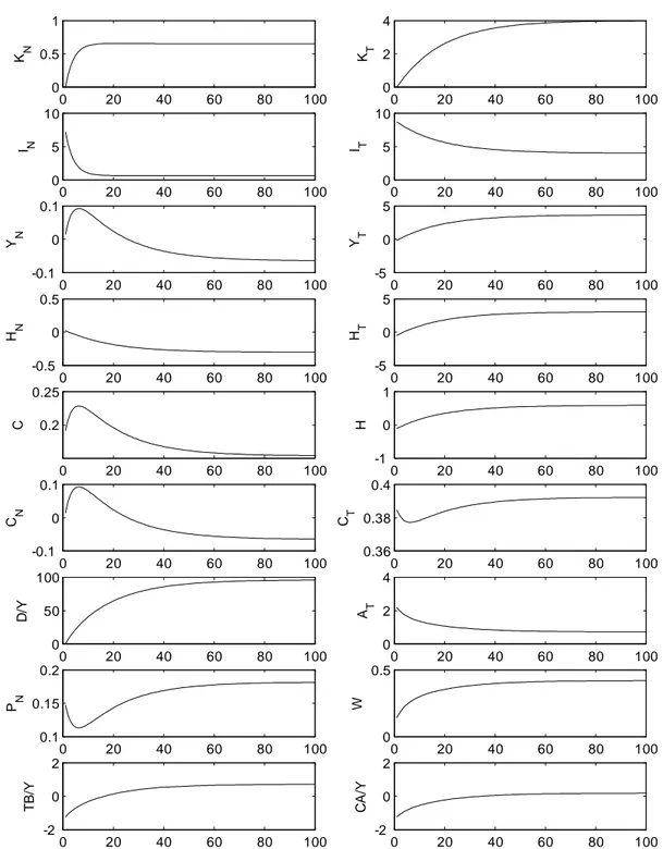
In this section we present results of simulations of the model under exogenous shocks: oil price shock and risk-premium shocks. We study a permanent, 1 percentage improvement in the price of oil, and a permanent, 1 percentage reduction in the risk-premium. Before examining the results of simulations of the model to these shocks, we brie‡y discuss the ‡exible analogue of the open-economy model and its responses to the same shocks. That provides a useful benchmark for the analysis of impulse responses of the model with sticky prices in the subsequent sections.
4.1 Flexible price equilibrium
The model collapses to the ‡exible price equilibrium in the case when …rms change their price with probability one, that is N = 1: We assume that in ‡exible price equilibrium there is no
distinction between backward-looking and forward-looking …rms, product markets are monopo-listically competitive and …rms set prices as a mark-up over marginal costs.
Monetary policy consistent with a ‡exible price equilibrium can be found by substituting the paths for in‡ation, t= 0; into the intertemporal relation (2.11). The interest rate instrument
of the central bank must satisfy it= rnt at all times, where:
1 + rnt+1 1fEt[
Ct Ct+1]g
1 (4.1)
rnt is the natural rate of interest, which is de…ned as the equilibrium real rate of return in the case of fully ‡exible prices.
Figures 1-2 illustrate impulse responses of the ‡exible price equilibrium model to the oil and risk-premium shocks. It is worth noting that the ‡exible-price dynamics of the present model are fully equivalent to those of a RBC version of the current model considered in Kuralbayeva and Vines (2006). The important di¤erence between a RBC model and the ‡exible-price limit of the model considered here, as pointed out by Woodford (2003), is that product markets are competitive in the former, rather than monopolistically competitive in later case. In the RBC model, the marginal costs of production are the same for all …rms at all times, because inputs of production are purchased on the same competitive rental market. While, in the ‡exible price limit of the sticky price model, prices charged by …rms are the same, as well as the levels of production of each good, so that marginal costs are in fact the same for all …rms.
4.2 Flexible exchange rate regime
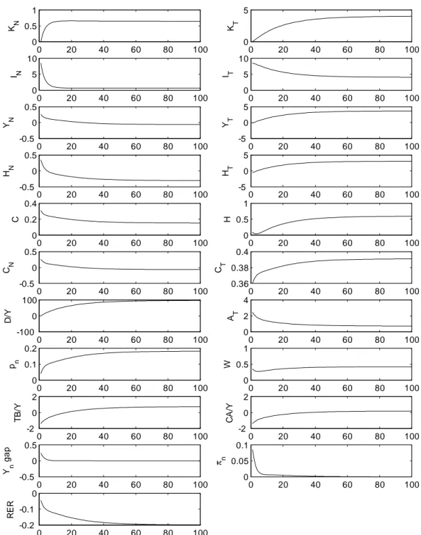
In this section we report results from simulations of the sticky-price model under a ‡exible exchange rate regime25.
4.2.1 Oil shock
2 5In impulse responses functions p
ndenotes relative price of the non-traded goods, while Pnis aggregate price
Figures 3-4 display impulse responses to the shock for the value ! = 0:01; while …gures 5-6 show the reaction of the variables to the shock in the case of ! = 0:9:
A positive oil shock increases demand for both non-traded and traded goods. As in the non-traded sector prices are sticky and output is demand-determined, the …rms that are not able to reset prices increase output as long as their prices are above marginal costs. This pushes demand for labor up. As no imperfections exist in the labor market, the nominal wage must increase. Due to the price stickiness, this generates an increase in the real wage. As real marginal costs increase on the impact of the shock, lucky …rms (those able to reset their prices) …nd it pro…table to set a price above the average price of the previous period. In setting their price, forward-looking …rms, due to the ‘front loading’ behavior, also take into account the future expected changes in real marginal costs. So, the price set by lucky …rms is above the average price that prevailed in the previous period, which causes an increase in the price of non-traded goods and in‡ation in that sector.
This is very di¤erent from what happens if in‡ation is almost entirely backward-looking. In that case the response of in‡ation is hump shaped. The reason for such di¤erent adjustment of in‡ation can be seen as follows. Because of the rule-of-thumb behavior, backward-looking …rms do not react contemporaneously to unexpected shocks. As a result, in‡ation rises only slightly on the impact of the shock. But as real marginal costs rises in the non-traded sector and some (even very small) fraction of forward-looking …rms set prices higher than in previous periods, in‡ation starts picking up in the non-traded sector in subsequent periods.
Under both cases the central bank accommodates the oil shock by increasing the (nominal) interest rate. The real interest rate also rises, given the Taylor principle. This monetary tighten-ing helps to suppress demand, directly via the real interest rate e¤ect and indirectly via its e¤ect on the real exchange rate. Both of these e¤ects curb in‡ation. There is a corresponding increase in the output gap, which causes additional monetary tightening and reinforces the interest rate e¤ect.
The nominal exchange rate appreciates on the impact of the positive demand shock. There-after, the higher interest rate results in a nominal depreciation of the exchange rate via the uncovered interest parity condition (UIP). The long-run depreciation of the nominal exchange rate is o¤set by an increase in the CPI price index of the same magnitude, so that in the long-run the real exchange rate moves back to its initial level. Thus, with an independent monetary policy the nominal exchange rate facilitates adjustment to the shock, which is re‡ected in a smooth movement of the real exchange rate back to equilibrium level.
Two further points about the behavior of the real interest rate and in‡ation are worth noting. First, in case of ! = 0:9; in‡ation slowly increases and then converges to its steady state at a very slow speed as well. It seems to peak about eight quarters after the shock. Second, despite very di¤erent dynamic responses of in‡ation and the (nominal) interest rate in the two cases, the real interest rate responses are very similar. This is because nominal interest rates closely follows the dynamics of in‡ation, and hence the real interest rate reaction in case of the accelerationist Phillips curve has the same pattern of behavior as in the case of the forward-looking Phillips curve. So, both real interest rates rise on the impact of the shock and then gradually converge to zero in the long-run. Given similar variations in the real interest rate, it is not surprising
that the reaction of real variables are very similar too. Moreover, those responses are much like that in the ‡exible price model. To see why it happens, consider the log-linearized version of the Euler equation (2.11):
bit+1= t+1+ ( bCt+1 Cbt) (4.2)
Given the de…nition of the natural rate of interest, one observes that the log-linearized version of the Euler equation (4.2) can be re-written as:
bit+1=brt+1n + t+1 (4.3)
The real interest rate that matters for the …rms in the non-traded sector is de…ned asbrt+1=
bit+1 N;t+1: Using the identity for aggregate in‡ation, t+1= N;t+1 (pbN;t+1 pbN;t); the real
interest rate faced by non-traded sector …rms can be related to the natural rate of interest in the following way:
brt+1=brnt+1 (pbN;t+1 pbN;t) (4.4)
where pbN;t is the log-linearized version of the relative price of the non-traded sector (pN;t =
PN;t=Pt): As identity (4.4) reveals the only time when there is a considerable di¤erence between
the real interest rate and the natural rate of interest is at the time of the shock, while at all other times the di¤erence pbN;t+1 (pbN;t+1 pbN;t) remains very small. So, in this model variations in
the monetary authority’s instrument track variations in the natural rate of interest, so that the real interest rate faced by the non-traded sector …rms is approximately equal to the natural rate of interest throughout the adjustment period to the shock. As discussed in Woodford (2003), such a Taylor rule policy, with characteristics above, would succeed in stabilizating in‡ation. As a result, the ‡exible price equilibrium is replicated here in the sense that real variables respond to the oil shock in a similar way to reactions of variables in the ‡exible-price model. In general, as noted by Woodford (2003), required variations in the natural rate of interest in response to the various types of shocks to replicate an equilibrium consistent with stable prices cannot be achieved through a simple Taylor rule. The assumption in our model, which is crucial in replicating the ‡exible price outcome, is ‡exibility of prices of traded goods. As shown in Smets and Wouters (2002), when prices of both sectors are sticky, there will be a trade-o¤ between stabilizing prices of domestic goods and stabilizing imported price in‡ation. If one of these two sectors is ‡exible, it is optimal for the central bank to stabilize in‡ation in the sector with sticky prices, and the ‡exible price equilibrium is replicated. This result is consistent with earlier work by Aoki (2001), who also …nds within two-sector model (a ‡exible price and sticky price sector, but without in‡ation inertia) that it is optimal to target in‡ation in the sticky-price sector, rather than to target aggregate in‡ation. When in‡ation is completely stabilized, the responses of the economy are equivalent to those of the ‡exible price model.
4.2.2 Risk-premium shock
Figures 7-8 present the impulse responses of the model to the shock for the value ! = 0:01; while …gures 9-10 illustrate the reaction of the variables to the shock for the value of ! = 0:9:
A permanent reduction in the foreign interest rate reduces the marginal costs of capital. Lucky …rms (who are able to reset their prices) …nd it pro…table to set a price below the average price of the previous period, which causes disin‡ation on the impact of the shock. In the case of backward-looking …rms, in‡ation rate does not react to changes in current real marginal costs, so in‡ation almost remains at its initial steady state level on impact of the shock.
After the initial response to the shock, in‡ation declines before increasing towards its new steady state level for both values of !. This is because (real) marginal costs are falling in the periods following the shock and then are increasing towards the new long-run equilibrium level. To explain this dynamic adjustment of in‡ation, we should notice that the outcome of the short-run is an increase in the return on capital in both traded and non-traded sectors, with a bigger increase on capital pro…tability in the non-traded sector.26 This rise of return on capital in the non-traded sector will cause capital in‡ow into the sector.
During some period following the shock the non-traded sector modi…es the optimal mix of factors of production in favor of more capital and less labor, so production costs fall. Given the reduction in (real) marginal costs, the price of non-traded goods is falling during that period. However, as the wage rate has been rising throughout the adjustment period, pressures that were making in‡ation fall will weaken. So, there will come a time when in‡ation starts rising again (although remaining negative) towards its new long-run equilibrium level. This process is slower in the case of the accelerationist Phillips curve compared to the forward-looking Phillips curve, given the rule-of-thumb behavior of backward-looking …rms.
Note that in the long-run in‡ation does not converge to its initial steady state level, which is di¤erent from the behavior of in‡ation in the long-run in response to an oil shock. The reason is that we now consider a permanent risk-premium shock, which changes marginal costs of production.
As in‡ation is negative throughout the adjustment period as well as in a new equilibrium, prices are falling permanently. Thus the real exchange rate appreciation occurs via appreciation of the nominal exchange rate, which o¤set the decline in the price level. Correspondingly, the burden of real exchange rate adjustment is taken by nominal exchange rate with smaller increase in prices. A permanent, 1 percentage reduction in the risk-premium assumes near 1 percent permanent decrease in the foreign interest rate on external borrowings by the country. In the long-run interest rate falls by 4.2 percentage points in case of ! = 0:01 and by 4.5 percentage points in case of ! = 0:9, the nominal exchange rate appreciates via the UIP condition with a constant rate of appreciation of 3.2 percent and 3.5 percent per quarter respectively.
As in the case of oil shock, the reaction of all real variables, for both values of !, are very similar to ones in the ‡exible price equilibrium. The intuition behind this result follows that of the oil shock discussed earlier.
4.3 Fixed exchange rate.
In this section we report results from similar simulations with a …xed exchange rate. The capital-mobility condition is then simply it = iFt : Now a country must give up an independent
2 6
monetary policy to keep the exchange rate …xed. Note that in this section we separate discussion of the simulation results for the case of a backward-looking Phillips curve from a forward-looking Phillips curve, as they are very di¤erent in the case of a …xed exchange rate regime.
4.3.1 Oil shock
Forward-looking Phillips curve (! = 0:01)
There are two features of impulse response functions (IRFs) in the …xed exchange rate regime, compared to ‡exible exchange rate regime, which are worth noting. First, short-run reactions of real variables and in‡ation are stronger in the …xed exchange-rate regime. Second, responses of real variables (except capital and investment in the non-traded sector) are hump shaped. The reason for such di¤erent propagation of the oil shock in the …xed exchange rate case can be seen as follows.
Given that the domestic interest rate is tied to the foreign rate and the fact that in‡ation rises on the impact of the shock, there is no short-run increase in the real interest rate in the country, as there was when the exchange rate could adjust. In fact, the real interest rate declines. An initial drop in the real interest rate stimulates investment in the non-traded sector, and this is a reason for the stronger increase in investment in the non-traded sector in the …xed exchange rate regime.
From households’side, the spending e¤ect of a permanent rise in oil transfers is bigger in the …xed exchange rate case. Under a ‡exible exchange rate regime, the positive oil shock produces a considerable nominal appreciation, which has a signi…cant impact on the spending e¤ect of the shock. The spending e¤ect (and thus consumption) is lower in the ‡exible exchange rate case than in the …xed exchange rate because increased demand for domestic currency is partly met through changes in the nominal exchange rate.
Higher demand for non-traded goods in the …xed exchange rate case generates stronger demand for labor, which pushes wages higher compared with the ‡exible exchange rate case. As wages rises more, real marginal costs increase more and the prices set by lucky …rms are higher, which causes a bigger initial jump in in‡ation in the …xed exchange rate case compared with the ‡exible exchange rate regime.
The initial e¤ects of the demand shock are larger on in‡ation in case of a …xed exchange rate compared with a ‡exible exchange rate. This is because part of the adjustment takes place via a change in the nominal exchange rate if the exchange rate is ‡exible.
In order to examine adjustment dynamics in response to the shock, we focus on three key elements of the adjustment process: the real interest rate, the real exchange rate, and the nominal exchange rate. As we discussed earlier, the real interest rate falls on the impact of the shock, which puts upward pressure on output in the non-traded sector. However, forward-looking behavior implies that the real interest rate is expected to be higher in subsequent periods, as they know the long-run value of the price level and expect prices to fall. So, in‡ation jumps up on the impact of the shock and then gradually falls as more and more price-setters adjust their prices to the new optimal level. The real interest rate is negative on the impact of the shock, but then starts rising, having a stabilizing e¤ect. Moreover, there is another stabilizing channel, coming from real exchange rate.
As in‡ation remains positive throughout the adjustment period towards the long-run equi-librium level, the country’s price level rises for some time and its real exchange rate declines (appreciates) for some time. This causes deterioration in net exports that results in a fall in demand for non-traded output. When demand falls low enough (precisely at the moment when the real interest rate returns to zero), prices start falling, and real exchange rate start depre-ciating. From here onwards, the dynamics of real variables are shaped by real exchange rate behavior only. Depreciation of real exchange rate will cause an improvement in net exports and that will cause an increase in the demand for non-traded output. Output increases gradually towards its long-run value. This explains the hump-shaped reaction of output in response to the shock. Similarly, hump-shaped responses of all other real variables are consequences of the same type of hump-shaped response of the real exchange rate. Such behavior of the real exchange rate is a result of the third channel of the adjustment process, or actually its absence: the nominal exchange rate. As discussed above, with an independent monetary policy with sticky prices, the nominal exchange rate carries out the burden of adjustment, resulting in a smooth response of the real exchange rate. In contrast, with a …xed exchange rate, prices do all the adjustment, which causes equivalent changes in the real exchange rate, re‡ected in a less smooth reaction of the latter. But because prices are sticky, an equivalent change in the real exchange rate would not be quick and immediate. This results in the hump-shaped behavior of the real exchange rate. For example, if prices were ‡exible, then the …xed exchange rate would be irrelevant since the relative price adjustment could be achieved by changes in prices and the real exchange rate would display the same pattern of response as in the ‡exible price model.
Backward-looking Phillips curve (! = 0:9):
The main feature of adjustment when there is a high proportion of backward-looking …rms is that it is slow and cyclical.27 The oscillations of the series of the non-traded sector are due to the evolution of backward-looking prices during the adjustment period towards steady state and the …xed exchange rate regime assumption. As we have seen above, backward-looking behavior does not modify signi…cantly the responses of the economy to the shocks in the case of a ‡exible exchange rate regime. However with commitment to the …xed exchange rate, the country gives up independent monetary policy and backward-looking behavior changes the adjustment dynamics of the economy to the shock considerably.
To understand oscillatory responses to the shock, as before, we focus on three key elements of the adjustment mechanism: the real interest rate, the real exchange rate, and the nominal exchange rate. As the output gap is positive on the impact of the shock, in‡ation starts rising gradually (because of inertia) and the real interest rate starts falling for some time. This falling real interest rate would cause further output gains which could push prices further up and in turn cause the real interest rate to fall further, and so on. This could be destabilizing. This destabilizing real interest rate mechanism has become known as ‘Walters critique’, because of
2 7
Cycles are not desirable because they imply high welfare losses for the economy. In this paper we do not perform welfare analysis. However, within the context of EMU, Kirsanova et. al. (2006) derive a welfare function with second and higher order terms of variables, from which it implies that cyclicality will result in a higher welfare loss. This is consistent with Leitemo (2002), who evaluates social loss under di¤erent targeting regimes and varying degress of in‡ation persistence for an open-economy (within one-sector model) and …nds that social loss is lower when there is less in‡ation persistence for most regimes considered.
the name of Sir A. Walters, who drew attention to the potentially destabilizing real interest rate response at the time when the UK entered the ERM.
However, the real exchange rate channel outweights the destabilizing e¤ect coming from real interest rate movements. Temporary real appreciation, initially very sluggish, is great enough to stabilize the economy. Comparison of the paths of the real exchange rate in the face of oil shock in …gures 6 and 14 con…rms that the real exchange rate appreciates more in the case of a …xed exchange rate regime than in a ‡exible exchange rate case. So, real exchange rate appreciation reduces demand, by having a stronger e¤ect than the real interest rate and demand starts falling after initial increase.
In addition, the presence of forward-looking …rms (though a small proportion) can reinforce the stabilizing real exchange rate e¤ect on the economy. This is because forward-looking con-sumers know that, as prices of non-traded goods are anchored by the price level outside the country, and if prices rise they would need to fall again, which would in due course cause the real interest rate to increase again. That would lead them to reduce their expenditure and thus demand. Thus, forward-lookingness in price setting helps to prevent instability coming from the real interest rate channel. The higher proportion of forward-looking …rms, the lower conse-quences of the destructive Walters e¤ects and a more smooth adjustment path. That is why, in most earlier papers on monetary policy in small open economies the ‘Walters critique’problems are absent, because these papers assume forward-looking wage and price setters.
A gradual rise in in‡ation causes an increase in the price of non-traded goods, which will reach a level high enough to reduce demand and cause the output gap return to zero. However, at this point prices are still rising because of the rule-of-thumb behavior of backward-looking …rms. This will lead to a further decline in the demand for non-traded goods, which will cause a further fall in the output gap. The output gap falls substantially causing a fall in the price of non-traded goods, and thus leading to a decline in in‡ation so that in‡ation reaches its long-run equilibrium level. However, at this point the output gap is below its potential level, so with an accelerationist Phillips curve28 it is necessary for the in‡ation rate to fall further, and in‡ation will start falling below the steady state level. This explains the oscillatory response of the economy to an oil shock in the case of a …xed exchange rate regime. As in the case of the forward-looking Phillips curve discussed earlier, in the absence of a ‘shock absorbing’role of the nominal exchange rate, the real exchange rate facilitates adjustment to the shock, resulting in an oscillatory reaction.
It is necessary to note that the problem of adjusting to the external shocks in a small open economy with …xed exchange rate and with a high proportion of backward-looking consumers and investors is similar, in many respects, to the problems faced by a small open economy with high degree of backwardness in the Phillips curve in responding to shocks in the monetary union. Westaway (2003) examines the key adjustment mechanisms available for a country in face of shocks inside and outside of monetary union. Our paper, in may respects, follows the same line of analysis. For example, our …ndings agree with his results, which show that no cycles are ensuing in a country with an independent monetary policy. Similarly without an independent
2 8
Under accelerationist Phillips curve, t= t 1+ &gaptin‡ation tends to rise when output is above potential
monetary policy, Westaway …nds that output and the real exchange rate would follow a more oscillatory path compared to outside.
4.3.2 Risk-premium shock
Forward-looking Phillips curve (! = 0:01)
The short-run e¤ects of the risk-premium shock is stronger in a …xed exchange rate regime compared with a ‡exible exchange rate. The intuition behind this result is similar to the case of the oil shock with a …xed exchange rate regime discussed earlier.
There is a stronger reaction of in‡ation to the shock compared with a ‡exible exchange rate. It is also should be noted that in‡ation behaves di¤erently in the long-run from what would happen if the exchange rate was ‡exible. In that case in‡ation decreases in the new steady state. In the …xed exchange rate regime, in‡ation converges to its initial steady state level. The reason is that to keep the exchange rate …xed, in the new steady state the domestic interest rate must fall by the magnitude of the shock to remain tied to the world interest rate, while in‡ation anchored by the outside’s in‡ation, goes back to its initial level.
Backward-looking Phillips curve (! = 0:9):
As in the case of an oil shock, a high proportion of backward-looking …rms implies an oscillatory reaction of variables of the non-traded sector. The responses of these variables are modi…ed by the rule of thumb behavior of backward-looking …rms and should be analyzed in the same way as in the case of the oil shock above. In contrast to the ‡exible exchange rate case, in‡ation converges to its initial equilibrium level as the interest rate and in‡ation are tied to the world interest rate and foreign in‡ation in case of the …xed exchange rate.
5
Conclusion
The debate regarding the choice of exchange rate for an open economy has not yet been closed. In the presence of nominal rigidities, the conventional wisdom is that a ‡exible exchange rate regime is preferable to the …xed rate in the face of real shocks. A freely ‡oating exchange rate serves as a real shock absorber, accommodating the needed adjustment in the real exchange rate without major real e¤ects.
This paper attempts to shed light on one aspect of this debate. In a dynamic general equilibrium model with endogenous in‡ation persistence, we study the question of insulating properties of the alternative exchange rate regimes in response to terms of trade and risk-premium shocks. We show that the country’s adjustment paths are slow and cyclical if there is a signi…cant backward-looking element in the in‡ation dynamics with a …xed exchange rate. Such adjustment dynamics are moderated if there is a higher proportion of forward-looking price setters. In the case of an almost entirely forward-looking Phillips curve, the responses of variables become hump-shaped. The reason is that with a …xed exchange rate, prices do all the adjustment, which causes equivalent changes in the real exchange rate. But because prices are sticky, an equivalent change in the real exchange rate would not be quick and immediate. This results in the hump-shaped behavior of the real exchange rate as well as other real variables of the model.