Trajectories and predictors of growth and neurodevelopment in Very Low Birth Weight infants

(1)

1

Alma Mater Studiorum – Università di Bologna

DOTTORATO DI RICERCA IN

SCIENZE MEDICHE GENERALI E SCIENZE DEI SERVIZI

Ciclo XXVI

Settore Concorsuale di afferenza:

06/M1 – IGIENE GENERALE E APPLICATA E STATISTICA MEDICA Settore Scientifico Disciplinare di afferenza:

MED/01 – STATISTICA MEDICA

TITOLO TESI

Trajectories and predictors of growth and neurodevelopment

in Very Low Birth Weight infants

Presentata da: Dott. Dino Gibertoni

Coordinatore Dottorato Relatore

Prof. Nicola Rizzo Prof.ssa Maria Pia Fantini

(2)

(3)

3

Il faut se tromper, être imprudent. Les hommes prudents sont des infirmes. (Jacques Brel)

(4)

(5)

5

ACKNOWLEDGMENTS

Several are the people to whom I owe a debt for helping me carry out this study. First of all drs. Silvia Vandini and Silvia Savini, who provided me data, feedbacks on the manuscript drafts and most of all who were patient enough to fulfill all my requests of data revisions and of explanations on the clinical and psychological processes of preterm children. For data correction, a big acknowledgement goes to dr. Mariangela D’Antuono. Profs. Giacomo Faldella, Alessandra Sansavini and Luigi Corvaglia supported from the beginning the challenge to apply some new statistical techniques to their workfield. Last but not least, prof. Maria Pia Fantini and dr. Paola Rucci supervised the study and succeeded in make things going – not only for this final dissertation but for all the Doctorate’s three years.

(8)

8

ABSTRACT

Neurodevelopment of preterm children has become an outcome of major interest since the improvement in survival due to advances in neonatal care. Many studies focused on the relationships among prenatal characteristics and neurodevelopmental outcome in order to identify the higher risk preterms’ subgroups. The aim of this study is to analyze and put in relation growth and development trajectories to investigate their relationship.

346 children born at the S.Orsola Hospital in Bologna from 01 January 2005 to 30 June 2011 with a birth weight of <1500 grams were followed up in a longitudinal study at different intervals from 3 to 24 months of corrected age. During follow-up visits, preterms’ main biometrical characteristics were measured and the Griffiths Mental Development Scale was administered to assess neurodevelopment. Latent Curve Models were developed to estimate the trajectories of length and of neurodevelopment, both separately and combined in a single model, and to assess the influence of clinical and socio-economic variables.

Neurodevelopment trajectory was stepwise declining over time and length trajectory showed a steep increase until 12 months and was flat afterwards. Higher initial values of length were correlated with higher initial values of neurodevelopment and predicted a more declining neurodevelopment. SGA preterms and those from families with higher status had a less declining neurodevelopment slope, while being born from a migrant mother proved negative on neurodevelopment through the mediating effect of a being taller at 3 months. A longer stay in NICU used as a proxy of preterms’ morbidity) was predictive of lower initial neurodevelopment levels.

At 24 months, neurodevelopment is more similar among preterms and is more accurately evaluated. The association among preterms’ neurodevelopment and physiological growth may provide further insights on the determinants of preterms’ outcomes. Sound statistical methods, exploiting all the information collected in a longitudinal study, may be more appropriate to the analysis.

(9)

9

INTRODUCTION

The decline of mortality in preterm infants led many researchers to focus their studies on neurodevelopmental disabilities, that remain as a great burden on infants’ families and on health care systems. The incidence and the factors associated with neurodevelopmental disabilities have been investigated from a multiplicity of different viewpoints. Earlier studies,1 focusing on the role played by nutrition on weight gain during hospitalization, showed that enriched formula milk fed preterms had both faster weight gain and improved cognitive outcomes during infancy and school-age compared with preterms who were term formula fed. The relationship of faster weight gain and head growth during the NICU stay with higher cognitive scores was found also by Ehrenkranz et al.2 The link among nutrition, weight gain and neurodevelopment was explained by the evidence that preterms who had inadequate nutrition in their early days were exposed to higher risks of infection and comorbidities, which in turn further delayed the achievement of an optimal nutrient level. The result is a reduced child’s overall health and energy level, that may lead to a lower neurodevelopment.2

These studies were generally conducted using as predictors clinical and anthropometrical variables collected only during the NICU stay and as outcomes the neurodevelopmental scores assessed at 18-22 months of life or later at school age. More recently, Belfort et al.3 pinpointed that a limitation of those studies was the wide temporal window among the outcomes and the explanatory variables, therefore ignoring the effect of mediating factors that may intervene during the post-NICU preterms’ development. The same authors importantly underline that, as a consequence, this leads to ignoring the association among development and socio-economic factors that may play a role mainly after discharge, when preterms’ caretakers are mostly members of their family environment.

Hence, the availability of data spanning the initial months of life of preterms after hospital discharge is not sufficient to ensure a comprehensive understanding of the mechanisms underlying the developmental process. Appropriate study design and statistical methods may actually provide a considerably better insight into this fundamental phase of preterms’ life.

(10)

10

This study uses Latent Curve Model analysis, a methodology that fully utilizes all available data, to attain three objectives:

• to obtain a model describing preterms’ neurodevelopment trajectory from 3 to 24 months of corrected age;

• to obtain a model describing preterms’ height growth trajectory from 3 to 24 months of corrected age; • to combine neurodevelopment and growth trajectories into a single combined model, describing the

relationships existing among the two patterns of change.

The models outputs include the shape and parameters of these growth trajectories, the effects of clinical and socio-economic predictors on the baseline levels and slopes of the two outcomes and lastly the degree of association among the height and neurodevelopment trajectories.

This study uses only height as a growth indicator but its replication substituting height with weight or cranial circumference is straightforward.

(11)

11

MATERIALS AND METHODS

Study population

The study population included ELBW (≤1000 g) and VLBW (≤1500 g) infants or infants born at less than 32 weeks of gestational age admitted at birth to the Neonatal Intensive Care Unit (NICU) of S.Orsola University Hospital, Bologna (North Eastern Italy) from 1/1/2005 to 06/30/2011, and enrolled in a follow-up program. Follow-up visits were made at 3, 6, 9, 12, 18 and 24 months corrected age; these specific time-points were chosen because they coincide with important milestones in the process of acquiring cognitive and functional abilities.

Written informed consent to participate in the study was obtained from parents. Data were anonymized prior to data analysis and the study protocol was approved by the local Ethics Committee.

Outcome measures of growth and neurodevelopment

The growth of newborns and specifically of preterm newborns has been quite extensively studied. A great effort has been made to set up longitudinal studies aimed to determine the standard trajectories of growth pattern for weight, length and cranial circumference. In these studies, different analytical and statistical criteria to summarize the results as well as different time points for the follow-up were considered.

A first distinction must be made among growth and catch-up growth. The term “catch-up growth” was introduced by Prader4 and Tanner5 in 1963 and was usually intended for height growth6; it describes the period of rapid linear growth in children that followed a period of growth inhibition, whose effect is to reconduce the children to their expected preretardation growth curve7. For preterm infants, it is referred to the early quick acceleration usually observed in SGA newborns. De Wit et al.6 argued that the correct measure for height catch-up growth is the standardized deviation score (SDS) and its change over time observed well beyond the first year life, because in that period this measure may be highly variable and still very dependent on the birth height. They

(12)

12

gathered information from previous studies showing that 80%-85% of SGA newborns recover in a normal height range in the first year of life, and that a similar result has been provided for preterms before the age of 3 years. In a very comprehensive paper, Sullivan et al.8 stratified a sample of 194 infants into five subgroups defined by SGA, term/preterm condition and presence/absence of comorbidities in preterms applying mixed effects linear models to test the differences in the group trajectories. Comparing infants on z-scores of weight, height and BMI over a long follow-up period until 12 years of age and using a set of biological and socio-cultural predictors to investigate the determinants of catch-up, they found that preterms had generally a steeper growth in the first 18 months but only some preterms groups reached the same growth as full-terms at 12 years of age. Therefore there is some evidence that a catch-up of length may be found not only for SGA but for VLBW preterms as well. However, since the aim of this study is not specifically focused on differences among SGA and non-SGA preterms, from now onwards the gain in length over time will be simply described as growth.

Neurodevelopment was evaluated using the revised Griffiths Mental Development Scale (GMDS-R, 0–2 years version).9 This scale consists of 276 dichotomous items that explore five functioning domains: Locomotor, Personal-Social, Hearing and Language, Eye and Hand Coordination, Performance. The assessment of these five separate domains allows to understand whether a delay in neurodevelopment may be due to some specific cognitive area, thus allowing to obtain a detailed cognitive profile for each preterm. Raw and standardized scores for each domain and a composite raw (RGQ) and standardized General Quotient (GQ) were calculated. Raw scores are the number of items appropriate for the infant’s age that were met by the preterm at each administration; RGQ is the sum of the five raw subscales’ scores. In the absence of normalized scores for the preterm infant Italian population,10,11 standard scores were obtained using the tables of standardized scores for the English infants population.12 For each domain, standardized scores have mean=100 and sd=16, while GQ has mean=100.5 and sd=11.8. Comparison with the standard values allows to evaluate whether preterms’ competences are different, though the absence of normalized scores on the Italian population and possible biases on first months’ scores lead to a cautious approach in the interpretation of results.13 In this study, only the composite GQ and RGQ scores were analyzed, using the raw scores for the sample description and the

(13)

13

standardized scores as the repeated observed measures in the latent growth models. For descriptive purposes GQ was also classified into the following categories: normal development (GQ≥88.7), mild (-1 to -2 SD, corresponding to 88.6-76.9 GQ scores), moderate (-2 to -3 SD, corresponding to 76.8-65.1 GQ scores) and severe delay (<-3 SD, corresponding to GQ≤65).11

The test was administered by two psychologists with long-standing experience in developmental assessment.

Griffiths Scales have been used in several studies13 on preterms that examined the relation among neurodevelopment and gestational age11,14,15 or gender16 or to investigate prospectively the relation among neurodevelopment and subsequent cognitive assessments, as scholar age cognitive delay17 or intellective quotient at 42 and 66 months of age.18 Findings are of a positive association among gestational age and neurodevelopment at 24 months, with ELBW newborns showing the worst performances; prospectively, a low development score at 24 months was found to be predictive of impairment at school age.

From the statistical viewpoint, these studies did not always rely on methods that allowed a thorough utilization of data available at each time point. Specifically, Gutbrod,19 Rijken,20 Leppänen21 and Brandt22 tested the association between clinical predictors and growth or between preterms’ growth and national growth charts with separate analyses at each observed timepoint; Mercier23 evaluated the predictors of severe disabilities at 18-24 months of age, and Ehrenkranz2 tested the association among in-hospital growth velocity and neurodevelopmental and growth outcomes at 18 to 22 months. Other studies instead took advantage of all the available data by using MANOVA for repeated measures11 and mixed-effects linear regression3,8 to estimate the growth curve parameters. In our study, two different outcomes will be measured: the neurodevelopment and the length growth curves until 24 months of age. To obtain these estimates and to subsequently put them in relation the Latent Curve Models methodology was used.

(14)

14

Independent variables

Biometric and clinical characteristics of the preterms were collected during their stay in NICU and in the follow-up visits, as well as preterms’ parents socio-economic variables. Each of these variables may then be evaluated as a potential predictor of neurodevelopment and length trajectories.

The independent variables analyzed in this study are:

Gender has been studied as a predictor of growth with contrasting results. Similar growth patterns of height

among genders were found by Casey,24 Rijken20 and Sullivan,8 while Hack25 found better growth in females and Guo26 and Morris27 in males. As for neurodevelopment, both the studies of Ehrenkranz2 and Mercier23 showed an increased risk of severe disabilities for males at 18-24 months of corrected age.

Gestational age (GA) in weeks was based on the last menstrual period and first-trimester scan.

Small for gestational age (SGA) is a binary variable indicating whether newborns’ birth weight was below a

standardized score of -1.28, corresponding to the 10th percentile of the reference neonatal growth charts developed ad hoc for the Italian population of preterm infants.28 While it is known that being SGA is associated with a worse outcome in extremely preterm infants,29 its influence on neurodevelopment is controversial. A negative effect on neurodevelopment was found only when paired with insufficient postnatal growth30 but in other studies SGA infants were found to have a better 5 and 20 months neurodevelopment than AGA infants paired by birthweight19 or to have no effect on 5-year cognitive outcome.21

Length of stay in the NICU (HS) in days was used as a proxy of neonatal morbidity after conducting

preliminary bivariate linear regression analyses, showing that this variable was positively and significantly (p<0.05) associated with the following severe postnatal conditions: mechanical ventilation, chronic lung disease (oxygen need at 36 weeks postmenstrual age), early onset and late onset sepsis (including both culture proven or clinical sepsis), necrotizing enterocolitis (requiring surgery), severe intra-ventricular hemorrhage (grade 3 and 4 as classified by Papile et al.,31 including post-hemorrhagic hydrocephalus requiring surgery or periventricular leukomalacia, classified as the presence of periventricular cysts at any cranial ultrasound performed during

(15)

15

hospital stay) and severe rethinopathy of prematurity (stages 3 to 5 according to the International Committee for the Classification of Retinopathy of Prematurity).32

Mother’s age at birth was introduced as a potential predictor of neurodevelopment; a previous study33 showed that mother’s age was significantly associated with socio-economic status. A higher mother’s age, as well as other variables such as the number of siblings, may also be indicative of better caregiving skills.

Twins have usually a high incidence among preterms; a recent study34 found that twins had a higher risk of mortality than singletons and a slightly higher long-term risk of motor and neurodevelopmental deficencies. The variable was coded as 0 for singletons and 1 for twins.

Information on siblings was entered in the study with a dichotomous variable, indicating whether preterms were firstborns (coded 0) or had older siblings (coded 1). In previous studies35,36 a negative influence on neurodevelopment of having siblings was found, explained by mothers spreading their attention among more than one child, therefore allowing a lower responsiveness to children needs, when compared to firstborns’ mothers.

Migrant condition of the mother is a dichotomous variable (mother of Italian nationality vs. other nationalities)

that was included as an indicator of preterms’ socio-cultural environment. Migration to Bologna and to Italy is a quite recent phenomenon, originating mainly from developing countries and Eastern Europe and comprising by a large amount non-specialized workers. For these reasons, migrants often live in conditions of material deprivation (associated to poverty) and social deprivation (involving isolation and low levels of social cohesion) that are linked to a higher risk of a preterm birth.37 These conditions of deprivation may likely affect also the post-hospitalization phase, when preterms usually live with their family, whose care-providing ability may be impaired by factors like poor housing conditions and low fluency in Italian language.

Hollingshead Index (HI) is a well-established index of socioeconomic status that takes into account the

educational and occupational status of the preterms’ parents.38 A higher HI is directly related to higher educational and occupational status, that is believed to reflect acquired knowledges and skills. HI ranges from 0,

(16)

16

when both parents have no formal education and are unemployed or retired, to 66 when both parents share the highest educational (graduate degree) and occupational (higher executives or major professionals) levels. Widely used in psychometry, HI was employed in studies on preterm infants8 as a stratification variable.

Diet at discharge and at 3 months of corrected age was coded as maternal (own mother’s raw milk, either

given by bottle or directly from the breast), mixed and exclusive formula milk. Fortification of bottle-administered human milk was routinely done during hospitalization and recommended after discharge until the weight of 3.5 kg was achieved. When needed, “preterm formula” was used during hospitalization and “post-discharge formula” was recommended after “post-discharge until the weight of 3.5 kg was achieved.

Sustained human milk feeding until 3 months of age is a dichotomous indicator that takes value 1 when a

preterm was fed maternal or mixed milk both at discharge and at 3 months corrected age. The beneficial effects of raw human milk feeding on neurodevelopment are well-known; however in a recent study on preterms (Gibertoni) a significant positive association with neurodevelopment at 24 months corrected age was found only for preterms who were fed human milk until 3 months of corrected age.

Nursery school attendance is a dichotomous variable observed at 12, 18 and 24 months of preterms’ age stating

whether they were attending a nursery school. It was hypothesized that preterms’ attendance of an environment external to the family could be associated to a different neurodevelopment level (AMPLIARE).

Statistical analysis

The study sample characteristics were summarized with descriptive statistics that included mean ± standard deviation and median with interquartile range for continuous variables, absolute and relative frequencies for categorical variables. Bivariate relationships among predictors were analyzed using t-tests or chi-square tests or linear correlations, depending on the level of measurement of the analyzed variables.

To determine whether length of NICU stay (HS) is a proxy of newborns’ severity of illness, a series of bivariate linear regressions were carried out, where HS was the outcome and each complication was in turn the only predictor.

(17)

17

Latent Curve Models

1

As Preacher et al.39 clearly state in the Introduction of their book, “early approaches to investigating change [over time] were very limited in that (a) they focused exclusively either on group-level or on invidual-level growth and (b) they addressed only two occasions of measurement, resulting in data too impoverished to allow examinations of some of the most basic and interesting hypotheses of change over time”. The afore-mentioned shortcomings may be overcome by using Latent Curve Models (LCM), a class of statistical methods belonging to the Structural Equation Models (SEM) family. LCM are designed to deal with longitudinal data collected on a sample of individuals, allowing to make inferences both on the interindividual change and on the intraindividual change over time, furthermore investigating on the predictors of change. LCM possess all the advantages of SEM, such as the ability to deal effectively with missing data and comprehensive measures of model fit to the data. Maybe the greatest advantage of SEM and LCM, linking the statistical analysis to the theoretical speculation, is the extreme flexibility in model design.

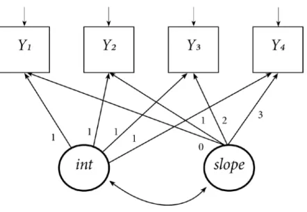
Several types of LCM of increasing complexity may be set up, depending on the hypotheses that can be made on the type of change. The simplest LCM is the Unconditional Linear Latent Curve Model (ULLCM), which considers the series of the observed values Yi as an expression of two latent growth factors, the starting level of the outcome measure (the intercept) and its linear growth rate (the slope). These factors are sometimes referred as the true initial measure and slope,40 because they represent estimates of the unknown corresponding values in the population. Since the growth curve estimated with an ULLCM is a straight line, this parameterization is suitable for outcomes that are supposed to change at a constant rate over time. In the ULLCM, the loadings from the latent intercept to the observed variables are all set to 1, because the intercept equally influences each observation; the loadings from the slope factor are set to a sequence of values that are proportional to the distance between the time points at which the observed variable was measured. By setting to 0 the loading from the slope to the first repeated measure, the intercept is assumed to estimate the mean value of y at the first

1

General references for the methodology of Latent Curve Models are the books by: Bollen and Curran69_{; Preacher, Wichman,}

(18)

18

assessment period. Each observed measure has an estimated residual, that is the part of variance that was not explained by the two growth factors. The parameters estimated by an ULLCM are:

• the mean intercept μα, which represents the mean initial level of the analyzed outcome; inference is made on μα to test the hypothesis that the mean intercept is different from 0;

Figure 1 –Diagram of an Unconditional Linear Latent Curve Model

the mean slope μβ, which represents the mean rate of change of the analyzed outcome per unit of time as defined by the lags on the loadings; inference is made on μβ to test the hypothesis that the mean growth rate is different from 0: should the null hypothesis be rejected, a significant increase or decrease was assessed; • the variance of the mean intercept ψα, which represents the variability of individual initial levels of the

outcome; inference is made on ψα to test the hypothesis that the individuals share the same initial level of the measured outcome;

• the variance of the slope ψβ, which represents the variability of individual rates of change in the outcome; inference is made on ψβ to test the hypothesis that the individuals share the same slope;

(19)

19

• the correlation between intercept and slope ψαβ, which represents the covariation among the growth factors; inference is made on ψαβ to test the hypothesis of a relation among starting values of the outcome and the growth rate.

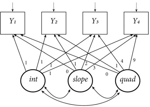
When a linear curve does not represent the data adequately, nonlinear models may be a better solution than ULLCM. Unconditional Latent Quadratic Curve Models (ULQCM) are an upgrade over ULLCM designed to produce a growth curve in a quadratic form. This type of curves are identified by two components: the linear component, that corresponds to the mean rate change, and the quadratic component, that corresponds to the acceleration (or deceleration if its parameter is negative) of the linear slope. Thus, ULQCM are well-suited to represent outcomes that have an initial steep increase followed by a stabilization as well as outcomes that have a later increase after an initial slow change. The curvilinear pattern is defined adding to the linear model a third latent variable that corresponds to the quadratic term and by setting its loadings on the observed values to the squares of the linear slope loadings.

(20)

20 Four more parameters need to be estimated in an ULQCM:

• the mean quadratic component μγ, which represents the degree of curvature rate in the trajectory; inference is made on μγ to test the hypothesis that the mean curvature rate is different from 0: should the null hypothesis not be rejected, then the model is equivalent to a linear model;

• the variance around the mean quadratic component ψγ, which represents the variability of individual curvature rates; inference is made on ψγ to test the hypothesis that the individuals share the same degree of curvature;

• the correlations between the mean quadratic component and the intercept (ψαγ) and between the mean quadratic component and the slope (ψβγ), which represent the covariations among curvature and the other growth factors; inference is made on these correlations to test the hypothesis of a relation among starting values of the outcome, growth rate and the curvature.

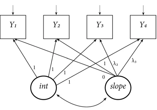
Another way to obtain nonlinear growth curves is to assume that the growth progression is not given a priori by setting each loading to a parameter corresponding to time lag between observations, but instead it is unknown and must be estimated by the model. This type of model is defined Unconditional Completely Latent Curve

Model (UCLCM)41,42 and is more exploratory than the previous models, because the researcher may gain insight into what trajectory might be the more appropriate to fit the data. Therefore an UCLCM may be well-suited for irregular trajectories that are of neither linear or quadratic shape and need to be evaluated point by point. To obtain an UCLCM (Fig.3) only two loadings from the slope to the observed values need be fixed: choosing to constrain the first to 0 and the second to 1 a metric of change was set and consequently the other loadings’ estimates reflect the cumulate proportion of change experienced until the corresponding timepoint compared to the change occurred between the first two observations.43 In an UCLCM the same parameters of an ULLCM needs to be estimated, plus the unknown loadings from the third (λ3, corresponding to the 9-months observation in this study) to the last observed measure (λ6, corresponding to the 24-months observation in this study).

(21)

21

Figure 3 –Diagram of an Unconditional Completely Latent Curve Model

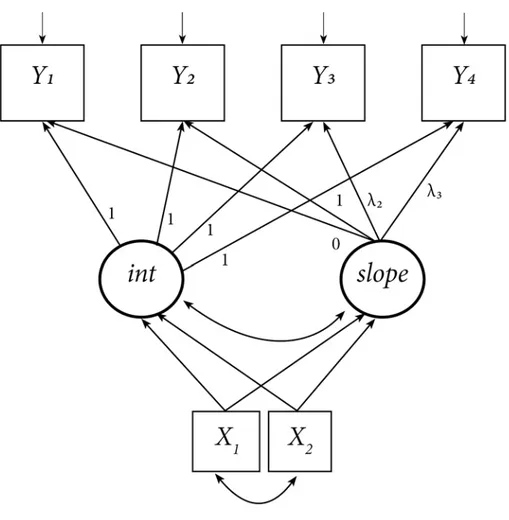
Each of the previously described models may be turned into a conditional model by adding at least one exogenous covariate. When the covariate does not change over follow-up time and it may theoretically be associated with at least one of the latent growth terms, then it is defined as a time-invariant covariate. This definition reflects that the covariate is a variable that may change among preterms but not over time and thus is supposed to influence just the mean baseline level and the mean growth rate and does not specifically affect the repeated observations. Typical time-invariant covariates are gender, gestational age or ethnicity. The association among time-invariant covariates and a latent growth factor is evaluated as a linear regression, therefore the strength of the association is measured by a regression coefficient and the usual inference on the coefficient’s significance is provided. Furthermore, by introducing time-invariant covariates the latent growth factors become dependent variables and consequently the estimation of their proportion of explained variance is made possible. Additional parameters to be estimated in a conditional model are:

(22)

22 • Residual variances of the growth factors;

• Correlations among the covariates (if specified).

Figure 4 –Diagram of a Conditional Latent Curve Model with time-invariant covariates

Alternatively or in addition to time-invariant covariates, time-varying covariates (TVC) may be added to a model. TVCs are variables measured simultaneously to the observed repeated measures, such as cranial circumference or nursery school attendance, and in an LCM are used as exogenous predictors of each corresponding wave of the observed variables. In this way, the explained variation of the observed repeated measures may be substantially improved. Differently from TICs, a TVC may change its effect on the outcome

(23)

23

over time, therefore an interesting result is the assessment of when the effect is significant and when it is stronger. TVCs are allowed to covary with the latent growth terms and with the TICs.

Figure 5 –Diagram of a Conditional Latent Curve Model with Time-varying covariates

Time-varying covariates are repeated measures themselves and rather than considering them as mere covariates it may be more helpful to view them as an outcome as well. In this way, a Parallel Process Model or

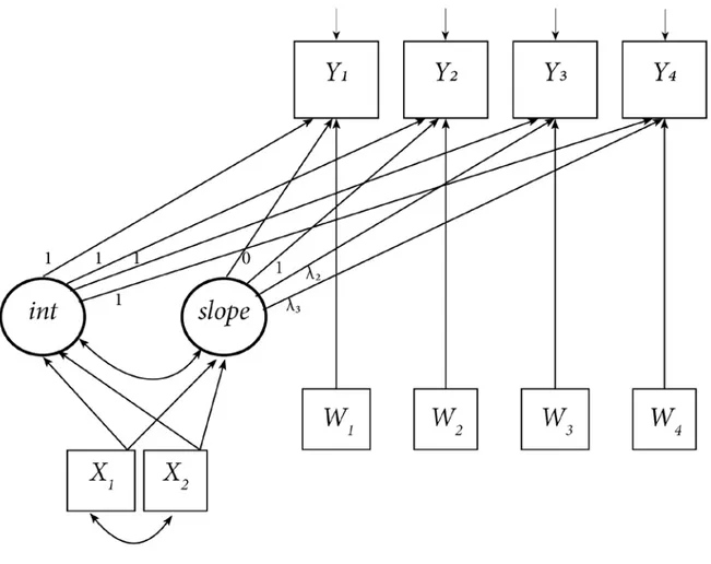
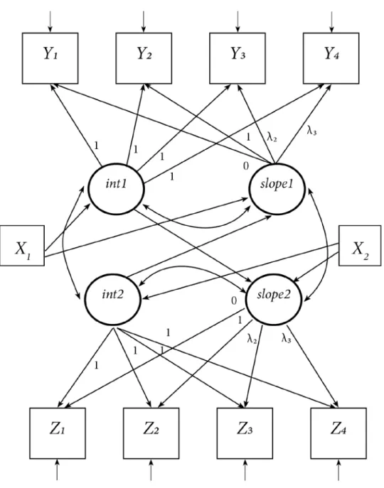
Multivariate Latent Curve Model (MLCM) that combines two different growth curves may be defined. The

advantage of MLCM is that causal relationships and covariations among the two sets of growth factors may be drawn and tested, allowing to investigate the relationships among aspects of change for different variables.42 For the evaluation of MLCMs it is advisable to work first on the single variable growth models and to join them only

(24)

24

after good solutions for both have been found. Parameter estimates of the joint model should not differ from those of the single models unless for different sample sizes due to to missing data. The researcher may then decide whether the two processes are simply related by adding covariations among the latent growth terms or they are causally related, by adding regression terms among the latent factors. With this latter choice it is possible for example to assess if the slope of one process may be predicted by the other process’ slope or mean initial value, and vice versa. A consequence of this choice is that the two latent intercepts may act as mediator variables between the independent covariates and the latent slopes: for instance, the effect of being SGA on the slope of neurodevelopment may be accounted as the sum of a direct effect and an indirect effect, passing through the initial level of length. It will then be possible to understand in a more accurate way the underlying processes that connect individual characteristics to the neurodevelopment curve.

(25)

25

Figure 6 –Diagram of a Multivariate Latent Curve Model with time-invariant covariates

Refinements of model estimation

Modifications to some of the parameters to be estimated are allowed in order to obtain a better fit or to resolve model identification issues. Means of the observed repeated measures should be constrained to lay on a straight

(26)

26

line (in the case of linear models) or on a parabola (in the case of quadratic models), but to improve model fit some of them may be freely estimated. This technique produces an estimated curve connecting with a straight line or a parabola each point except for those freely estimated, that will show as a bump in the curve. The estimated slope is then referred to the curve connecting all the constrained time points.

Similarly, all observed variables are constrained to have the same variance, but when actually one or some of them differ importantly, this may cause serious model identification problems due to the non-positive definite covariance matrix issue. To resolve this issue it is necessary to let the variance causing problems to be freely estimated, thus obtaining a better fit as well.

Model improvements of this kind are usually suggested by the values of model indices, that are estimates of how much model fit will improve whether a parameter is modified or added to the model. A high modification index is often a sign of model misfit. Typical modification to models are freeing a constrained parameter, adding a causal effect or adding a covariance among variables; however, these changes must always have a theoretical justification.

Another modification to data that is often necessary is related to the variance magnitudes. In LCM and more generally in every SEM model, if the ratio of the largest to the smallest variance of the variables included in the model exceeds 10, the covariance matrix is ill-scaled and may determine inaccurate estimates of the model fit, due to the iterative nature of the estimation process.44 This may very likely happen in conditional models, if continuous measures are evaluated together with dichotomous variables. To overcome this issue, the variable(s) with the higher variance(s) must be divided by a constant, transforming them at a smaller scale until their variance magnitude is comparable to the other variables’ variances.

Estimation of LCM and assessment of normality

Maximum Likelihood (ML) is the standard method used to provide LCM estimates. It has several desirable properties, such as consistency, asymptotic unbiasedness, asymptotic normality and asymptotic efficiency. Furthermore, the Full Information Maximum Likelihood (FIML) is recognized as the preferred method to deal

(27)

27

with missing data. The properties of the ML estimator are maintained when the observed variables (the repeated measures of GQ for models of neurodevelopment and the repeated measures of length for models of growth) have the same multivariate kurtosis as a multivariate normal distribution.45 Should this assumption be violated, biases may occur in the estimates of asymptotic standard errors and of significance test statistics. To verify the null hypotesis of multivariate skewness and kurtosis, tests proposed by Mardia46,47 were evaluated. In cases of violation of the normality assumption, the robust maximum likelihood (MLR) estimator is suggested; desirable properties of the MLR estimator are the standard errors and χ2

test statistic robust estimates provided in situations of non-normality, missing data and small to medium sample sizes.48,49

Model fit

Being part of the SEM family, Latent Curve Models provide an assessment of the overall model fit to the data. Model fit are summary measures that quantify the adherence of model estimated parameters to the variances, covariances and the means of the observed variables. Not only a good fit is a prerequisite for interpreting parameter estimates, but comparison of model fit is a straightforward criteria to select the more appropriate among alternative models. Several fit indices have been developed and no consensus on a single standard index was reached so far. Therefore, it is advisable to report different fit indices, since they represent different aspects of model fit to the data. For the assessment of a good model fit all reported indexes must have values comprised in the respective ranges of good or acceptable fit, while for comparison among models the best fitting model is identified when it has best values on possibly each fit index. In this study, five fit indices reported by Mplus were used to evaluate model fit:

Comparative Fit Index (CFI) compares the analyzed model with the null model which assumes zero covariances

among the observed variables.50 CFI ranges from 0 to 1 and when it reaches the cutoff value of 0.95 it indicates a good model fit.51

(28)

28

Tucker-Lewis Index (TLI) is another index usually reported along with the CFI that compares model fit to the

null model fit.52 It ranges from 0 to 1, with higher values indicating a better fit; a 0.90 cutoff is the least acceptable fit value.

Root Mean Square Error of Approximation (RMSEA) is a fit index with no baseline comparison that measures

average lack of fit per degree of freedom.53 It has no upper limit and a minimum of zero, which indicates the perfect fit. Cutoff values are 0.05 for a good fit and 0.10 for a moderate fit.54 The advantage of RMSEA is that in addition to the point estimate it provides the 90% confidence interval around its value and a close-fit test for the null hypothesis H0: RMSEA≤0.05. To ensure a good fit, the confidence interval should have its upper end below 0.8 and the close fit test should not be rejected (p should be >0.05).

Moreover, Akaike Information Criterion (AIC) and Bayesian Information Criterion (BIC) indexes are used to compare alternative models. These indexes are based on information theory approach and take into account both the goodness of fit and parsimony of a model. Models with smallest AIC or BIC values are those with a relatively better fit and fewer free parameters compared with competing models.

Sample size and missing values

Sample size is a critical issue in SEM and consequently in LCM, because a small sample size may lead to inaccurate estimates.44 There is no consensus upon a minimum standard sample size, because there are many features of LCM models that need to be taken care of. However, the most followed criteria is to look at the ratio

N/q between the number of cases and the number of free parameters that needs to be estimated. This rule can be

applied when the estimation method is maximum likelihood, but it depends also upon the non-normality of data. The higher the ratio, the better; however, general rules of thumb are that a minimum ratio of 5:1 may be good for normal multivariate data,55,56 while with strong kurtotic data the ratio should be at least in the order of 10:157 and an ideal ratio would be of 20:144. In the results section, along with the estimates, the N/q ratio will be provided for each tested model.

(29)

29

The standard method used in statistical inferential analysis to assess sample size adequacy is power analysis, but its application to SEM is awkward because it would require many distinct estimations that for complex models may result very challenging.58 Several approaches have been applied in order to adapt power analysis to SEM, one of which is the test of not close fit,59 based on an inference upon the RMSEA index: if the 95% confidence interval around the index is entirely below 0.05 then the model has a good fit because the hypotesis of not close fit is rejected. With this approach, a higher power value is related to a wider sample size and on a greater number of free parameters to be estimated. Applying the formulae exposed by Hancock and Freeman,60 an estimate of power based upon the test of not close fit has been provided for the simplest of the proposed models, taking into account that its estimated value of power should be the lower among all models. Estimates of power from 0.80 to 1 indicate an optimal sample size, while values in the range 0.60-0.80 indicate a sufficient sample size.

Some follow-up measures of preterms’ GQ score were missing for a number of reason, such as: unavailability of infants and parents at the requested follow-up time, follow-up visits made at an excessively delayed or anticipated time with respect to the scheduled date, impossibility to administer the test for infants’ illness. When causes of missingness do not seem to be related with the outcome, missing data may be considered missing at random (MAR) and estimation procedures can be applied to obtain a full data set.

Missing data estimation was made with the FIML, which is a highly reliable estimation method and is run simultaneously to the model estimation procedure. However, in order to limit the possible bias in missing data estimation, infants who were not seen on at least 3 out of the 6 occasions between 3 and 24 months were excluded from the analysis. To evaluate whether this criteria may cause a selection bias, a preliminar representativity analysis was carried out to compare the clinical and socio-demographic characteristics of infants who had at least 3 follow-up visits against those who had only 1 or 2 visits.

(30)

30

Development of Latent Curve Models

The last aim of the study was to analyze the relationship among the preterms’ neurodevelopment and length trajectories; to fulfill this aim, which is accomplished by evaluating a very complex model, a series of models progressively more complex have been defined and tested. Neurodevelopment and length latent curves were first estimated separately in order to find the best fitting univariate models and only at a final stage they were combined together in a multivariate LCM. At each stage, criteria to select the best model were the fit indices values and the clinical soundness of the results. Firstly, the most adequate unconditional model was selected by comparing linear, quadratic and completely latent models. The best fitting among these three models was then accrued into a conditional model with the addition of time-invariant and time-varying covariates, chosen among those that theoretically could influence the neurodevelopment or length trajectory. The best fitting model at the end of this stage was considered the best model for the single outcome of neurodevelopment or length. The two resulting models were then combined together in a multivariate LCM, that was nonetheless subject to modifications and alternative formulations, due to the likely different trajectories shapes and interrelations among factors and predictors.

Mplus 7.11 (Muthén & Muthén, Los Angeles, California, USA) was used for the estimation of latent curve models; all the other analyses were carried out using Stata 13.1 (StataCorp LP, College Station, Texas, USA).

(31)

31

RESULTS

Sample characteristics

The study has been carried on preterms born in the S.Orsola Hospital’s NICU starting from January, 1th 2005 until June, 30th 2011 and subsequently followed-up until June, 30th 2013, in order to have a potential 24-months follow-up interval for each preterm. The preterms recruited were 346; 22 (6.4%) were excluded from the analysis because they attended less than 3 follow-up visits. The main reasons for missing visits were newborn’s illness or family’s temporary unavailability. Excluded newborns were significantly different only for a larger cranial circumference at discharge (mean CC was 33.7 cm vs. 32.1 cm; t-test=2.624; p=0.009) and a higher weight at discharge (mean weight was 2359 gr vs. 2097 gr; t-test=2.978; p=0.003). However, the difference in standardized weight at discharge was not significant (mean z-score was -1.269 vs. -1.680; t-test=1.588; p=0.113). Gestational age (29.5 wks. vs. 29.1) and birthweight (1276.8 gr vs. 1161.8) were higher for the excluded newborns but without achieving statistical significance (t-test: p=0.344 and p=0.134 respectively). As a result, newborns excluded because they did not attend at least 3 follow-up visits were tendentially in better conditions but not so much as to lead to a possible selection bias.

Table 1 describes the preterms characteristics. The overall mean gestational age was 29.1 weeks, with the large majority of newborns being very preterm (28<=EG<=31 wks, 66.0%) or extremely preterm (EG<28 wks, 24.4%). The proportion of preterms who were SGA was 17.6%; SGA preterms had a significantly longer gestational age when compared to AGA/LGA preterms (t-test: t=-2.78; p=0.006), because for the sample selection criteria, which also included newborns with EG>32 weeks if they had birthweight under 1500 gr., all late preterms were SGA and 48.0% of moderately preterms were SGA. Complications and comorbidities had an incidence ranging from the 1.6% of ROP to the 20.7% of BPD. Length of stay in the NICU showed a great variability, ranging from a minimum of 6 days to a maximum of 223 days (mean stay was 58.6±34.3 days and the median stay was of 51 days). In bivariate linear regressions each complication proved to be significantly

(32)

32

associated with a longer NICU stay, as shown in Table 2. The type of feeding at discharge was human milk (own mother’s or mixed) for around 70%, and at 3 months it was 76.6%.

Tab.1 – Characteristics of the study sample (n=324)

PERINATAL AND CLINICAL

CHARACTERISTICS N (%) Mean ± Std. Dev Median ± IRQ Missing data n (%)

Gestational age (weeks) 29.1±2.4 -

Late preterm (34-36 w.) 6 (1.9) Moderately preterm (32-33 w.) 25 (7.7) Very preterm (28-31 w.) 214 (66.0) Extremely preterm (<28 w.) 79 (24.4) Twins 105 (33.0) 6 (1.9) Females 165 (50.9) - SGA 57 (17.6) - IVH or LPV 17 (5.3) - BPD 67 (20.7) 1 (0.3) Sepsis 48 (14.9) 1 (0.3) ROP 5 (1.6) 1 (0.3) NEC 13 (4.0) - Hospitalization (days) 58.6±34.3 4 (1.2) ELBW (<1000 gr.) 111 (34.3) - Weight at birth (gr.) 1161.8 ± 353.0 1191 ± 558 - Weight at discharge (gr.) 2097.3 ± 365.6 1980 ± 400 8 (2.5)

Weight at birth (z-score) -0.206 ± 1.00 -0.180 ± 1.44 -

Weight at discharge (z-score) -1.680 ± 1.17 -1.595 ± 1.48 8 (2.5)

Length at birth (cm.) 37.1 ± 4.4 38 ± 5.8 140 (43.2)

Length at discharge (cm.) 43.8 ± 2.7 44 ± 3 144 (44.4)

Cranial circ. at birth (cm.) 27.1 ± 2.8 27 ± 4 163 (50.3)

Cranial circ. at discharge (cm.) 32.1 ± 1.7 32 ± 2 141 (43.5)

Diet at discharge -

Own mother’s milk 109 (33.6)

Formula milk 98 (30.2)

Mixed milk 117 (36.1)

Diet at 3 months 29 (8.9)

Own mother’s milk 51 (17.3)

Formula milk 226 (76.6)

(33)

33

BIOMETRIC

CHARACTERISTICS Mean ± Std. Dev

Median, IQR Missing data, n (%) Weight at 3 months (gr.) 5451.6 ± 956.1 5530, 1205 15 (4.6) Weight at 6 months (gr.) 7063.5 ± 1119.0 7080, 1545 25 (7.7) Weight at 9 months (gr.) 8212.5 ± 1252.9 8290, 1675 49 (15.1) Weight at 12 months (gr.) 9106.3 ± 1309.1 9140, 1635 55 (17.0) Weight at 18 months (gr.) 10351.3 ± 1433.7 10400, 1755 52 (16.0) Weight at 24 months (gr.) 11535.0 ± 1648.0 11575, 2135 45 (13.9) Weight at 3 months (z-score) -0.765 ± 1.48 -0.662, 1.70 15 (4.6) Weight at 6 months (z-score) -0.776 ± 1.29 -0.751, 1.65 25 (7.7) Weight at 9 months (z-score) -0.706 ± 1.23 -0.637, 1.61 49 (15.1) Weight at 12 months (z-score) -0.708 ± 1.18 -0.685, 1.43 55 (17.0) Weight at 18 months (z-score) -0.784 ± 1.13 -0.765, 1.43 52 (16.0) Weight at 24 months (z-score) -0.725 ± 1.15 -0.714, 1.57 45 (13.9)

Length at 3 months (cm.) 58.3 ± 3.4 58.5, 5 45 (13.9) Length at 6 months (cm.) 65.4 ± 3.4 65.5, 4.3 46 (14.2) Length at 9 months (cm.) 70.3 ± 3.3 70.5, 4.3 47 (14.5) Length at 12 months (cm.) 74.4 ± 3.3 74.5, 4.5 57 (17.6) Length at 18 months (cm.) 80.7 ± 3.6 81, 4.5 52 (16.0) Length at 24 months (cm.) 86.3 ± 3.5 86.5, 4.2 46 (14.2) Length at 3 months (z-score) -1.000 ± 1.61 -0.850, 2.00 45 (13.9) Length at 6 months (z-score) -0.825 ± 1.48 -0.667, 2.02 46 (14.2) Length at 9 months (z-score) -0.452 ± 1.32 -0.292, 1.67 47 (14.5) Length at 12 months (z-score) -0.362 ± 1.28 -0.280, 1.60 57 (17.6) Length at 18 months (z-score) -0.433 ± 1.24 -0.352, 1.55 52 (16.0) Length at 24 months (z-score) -0.400 ± 1.12 -0.339, 1.33 46 (14.2) Cranial circ. at 3 months (cm.) 40.2 ± 1.7 40.4, 2.2 17 (5.2) Cranial circ. at 6 months (cm.) 43.1 ± 1.9 43.2, 2.4 46 (14.2) Cranial circ. at 9 months (cm.) 44.9 ± 1.9 45, 2.2 48 (14.8) Cranial circ. at 12 months (cm.) 46.1 ± 1.9 46.1, 2.4 55 (17.0) Cranial circ. at 18 months (cm.) 47.3 ± 1.9 47.3, 2.3 55 (17.0) Cranial circ. at 24 months (cm.) 48.2 ± 1.9 48.2, 2.3 46 (14.2) Cranial circ. at 3 months (z-score) -0.198 ± 1.35 0, 1.67 17 (5.2) Cranial circ. at 6 months (z-score) -0.272 ± 1.42 -0.167, 1.81 46 (14.2) Cranial circ. at 9 months (z-score) -0.299 ± 1.37 -0.154, 1.77 48 (14.8) Cranial circ. at 12 months (z-score) -0.273 ± 1.36 -0.231, 1.85 55 (17.0) Cranial circ. at 18 months (z-score) -0.457 ± 1.34 -0.357, 1.77 55 (17.0) Cranial circ. at 24 months (z-score) -0.517 ± 1.31 -0.407, 1.74 46 (14.2)

(34)

34 DEVELOPMENTAL CHARACTERISTICS Mean ± Std. Dev Median, IQR Missing data, n (%)

Griffiths raw score at 3 months 53.2 ± 7.8 54, 9 14 (4.3) Griffiths raw score at 6 months 98.3 ± 12.9 100, 15 15 (4.6) Griffiths raw score at 9 months 137.6 ± 13.6 139, 15 14 (4.3) Griffiths raw score at 12 months 169.6 ± 15.6 172, 14.5 16 (4.9) Griffiths raw score at 18 months 217.1 ± 22.0 220, 22 35 (10.8) Griffiths raw score at 24 months 251.5 ± 19.9 256, 17 35 (10.8) Griffiths score at 3 months 113.1 ± 10.6 115, 10 14 (4.3) Griffiths score at 6 months 107.1 ± 12.3 109, 13 15 (4.6) Griffiths score at 9 months 107.1 ± 12.6 108, 16 14 (4.3) Griffiths score at 12 months 102.5 ± 12.7 104.5, 14 16 (4.9) Griffiths score at 18 months 94.1 ± 14.5 96, 17 35 (10.8) Griffiths score at 24 months 93.9 ± 15.1 97, 18 35 (10.8)

OTHER

CHARACTERISTICS N (%) Mean ± Std. Dev Missing data, n (%)

Number of siblings 0.3 ± 0.6 2 (0.6)

Age of mothers 33.8 ± 5.4 3 (0.9)

Educational level of mother 16 (4.9)

low 60 (19.5)

intermediate 146 (47.4)

high 102 (33.1)

Educational level of father 23 (7.1)

low 71 (23.6)

intermediate 135 (44.8)

high 95 (31.6)

Hollingshead Index 35.1 ± 10.7 15 (4.6)

Migrant mothers 78 (24.1) 1 (0.3)

Nursery school attendance at

12 months 6 (2.5) 86 (26.5)

18 months 32 (13.1) 80 (24.7)

(35)

35

Tab.2 Bivariate linear regressions of length of stay in NICU (days) on the presence of complications

Constant b std err. (b) p N

Intra-Ventricular Hemorrhage /

Periventricular Leukomalacia 56.604 38.043 8.29 <0.001 319 Mechanical Ventilation 45.634 50.695 3.36 <0.001 320 Broncho Pulmonary Displasia 46.635 56.246 3.49 <0.001 319

Sepsis 51.782 44.301 4.75 <0.001 319

Retinopathy of Prematurity 57.350 70.050 14.93 <0.001 319 Necrotizing Enterocolitis 56.189 59.965 9.13 <0.001 320

Patterns of change of biometric and neurodevelopmental measures

Change in the main biometric measures (weight, length and cranial circumference (CC)) from birth to discharge show a relevant increase in absolute values and a corresponding large decrease in variability (as observed with median ± IQR that are less sensible to extreme values). This was mainly caused by SGA, who gained on average 1010 gr. and whose IQR reduced from 547 to 300 gr, compared with a corresponding average weight increase of 791 gr and IQR 158 gr reduction for AGA-LGA. However, such a result may be mainly attributable to the significantly longer NICU stay of SGA newborns (71.2 vs. 56.0 days, t-test=-3.01, p=0.003).

As for the socio-economic characteristics of newborns’ family environment, infants in our study were generally firstborns (77.0%) and only 4.3% had two or more elder siblings. Mean and median age of mothers was around 34 years, with a wide variation spanning from 18 to 47 years. Infants born from migrant mothers were 78, with 31 different foreign countries of origin; the more frequent of these were Eastern European countries (Romania, Moldavia, Albania), Nigeria and some Asian countries (Bangladesh, Pakistan). The proportion of preterms with a migrant mother (24.1%) is not much higher than that of newborns in the Bologna province in the years 2005-2011 (23.3%)2. Compared to infants born from Italian mothers, a higher proportion of preterms from migrant mothers had siblings (30.8% vs. 20.8%) and their mean mothers’ age was lower (31.4 vs. 34.5 years). Education

(36)

36

level of mothers and fathers was intermediate-high, since a low-level of education was reported by about 20% of parents. Among migrant mothers there was a lower proportion of graduates (25.6% vs 33.5%) and a higher proportion of mothers whose educational level was unknown or elementary school level (14.1% vs 3.7%). The Hollingshead Index (HI) was significantly lower when the mother was migrant compared to when the mother was Italian (mean HI 29.1 vs. 37.2; t-test: t=6.21; p<0.001). There was no association among HI and firstborn condition of the infants: mean HI for firstborn’s parents was 35.2 compared with 35.0 for non-firstborn’s parents (t-test: t=0.158; p=0.875), while there was a moderately significant positive correlation (r=0.295; p<0.001) between HI and mother’s age. Infants’ attendance of nursery school began at the age of 12 months (6 infants, 2.5% of the total), with a growing proportion of attendance at 18 months (12.4%) and at 24 months (33.2%). Nursery school attendance did not differ significantly between infants born from migrant and non-migrant mothers, both at 18 months (19.2% vs. 11.5%; χ2_{=2.13, p=0.145) and at 24 months (41.3% vs. 31.2%; χ}2

=1.66, p=0.197). Similarly, HI did not differ significantly between newborns attending and not attending nursery school, both at 18 months (37.5 vs 35.1; t-test=-1.16, p=0.246) and at 24 months (36.6 vs. 34.4; t-test=-1.43, p=0.155).

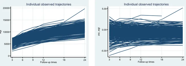
Biometric characteristics measured at follow-up waves (weight, length and cranial circumference at 3, 6, 9, 12, 18 and 24 months corrected age) all show a positive growth pattern in absolute values but with regard to standardized scores the patterns were different. Weight in absolute value increases at a high rate in the first followup interval and then progressively decelarates. The individual observed trajectories of weight represented in Figure 7 follow an increasing slightly curvilinear pattern, while in the individual observed trajectories of standardized weight (Figure 8) a ‘funnel’ pattern from 3 to 6 months may be observed, related to a reduction in scores’ variability (sd decreases from 1.48 at 3 months to values around 1.2 in all the following waves). However, preterms remain underweight during all follow-up period, with means of weight z-scores floating around -0.75.

(37)

37

Figure 7 –Trajectories of weight between 3 and 24 months corrected age; absolute values’ trajectories

Figure 8 –Trajectories of weight between 3 and 24 months corrected age; standardized scores’ trajectories

Length’s growth (Figure 9) follows a pattern similar to the weight pattern for absolute values, but with an increase that looks steeper in the first months and a more marked curvilinear form. The corresponding z-scores trajectories (Figure 10) show an initial increase and a reduction in variability followed by a stabilization on negative values around -0.40 after the 9-months visit.

Figure 9 –Trajectories of length between 3 and 24 months corrected age; absolute values’ trajectories

Figure 10 –Trajectories of length between 3 and 24 months corrected age; standardized scores’ trajectories

Cranial circumference growth pattern was quite different (Figures 11 and 12). Until the 9-months visit its increase in absolute values was much steeper than the one found for weight and length, but afterwards it changed into a flatter one, thus defining an evident curvilinear shape. The trajectories of cranial circumference

0 5000 10000 15000 20000 w gt 3 6 9 12 18 24 Follow-up times

Individual observed trajectories

-5.00 0.00 5.00 zsc_ w g t 3 6 9 12 18 24 Follow-up times

40 60 80 100 lgt 3 6 9 12 18 24 Follow-up times

-10.00 -5.00 0.00 5.00 zsc_ lg t 3 6 9 12 18 24 Follow-up times

(38)

38

standardized scores were slowly but constantly declining over time, with a change from a mean z-score of -0.198 at 3 months to a mean z-score of -0.517 at 24 months.

Figure 11 –Trajectories of cranial circumference between 3 and 24 months corrected age; absolute values’ trajectories

Figure 12 –Trajectories of cranial circumference between 3 and 24 months corrected age; standardized scores’ trajectories

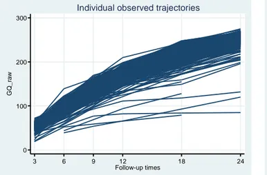
Neurodevelopment measured by the Griffiths raw scores (Figure 13) had a constant and slightly curvilinear increase, with most preterms following a similar pattern and a few of them remaining at lower values with a flatter curve. Looking at standard scores (Figure 14), the pattern is that of a constant decrease until 18 months.

Figure 13 –Trajectories of neurodevelopment between 3 and 24 months corrected age; raw scores’ trajectories

Figure 14 –Trajectories of neurodevelopment between 3 and 24 months corrected age; standard scores’ trajectories

30 35 40 45 50 55 cc 3 6 9 12 18 24 Follow-up times

-6.00 -4.00 -2.00 0.00 2.00 4.00 zsc_ cc 3 6 9 12 18 24 Follow-up times

0 100 200 300 G Q_ ra w 3 6 9 12 18 24 Follow-up times

40 60 80 100 120 140 GQ 3 6 9 12 18 24 Follow-up times

(39)

39

Latent curve models

Models based on repeated measures of neurodevelopment (GQ)

The following models are estimated using repeated measures of neurodevelopment taken at 3, 6, 9, 12, 18 and 24 months of age. All neurodevelopment observed variables (GQ3 to GQ24) were rescaled dividing by 10, in order to solve an ill-scaled variances issue. As a consequence, the estimates of the latent intercept should be multiplied by 10 to return to the original GQ scale when interpreting the results.

Assessment of normality assumption

The assessment of multivariate normal assumption using Mardia’s multivariate skewness and kurtosis tests resulted in the rejection of the null hypotesis (for both p<0.001), meaning that for the observed repeated measures of neurodevelopment the assumption of normality was violated. To cope with the possible bias on significance test statistics caused by non-normality, estimates were carried out using the robust maximum likelihood estimator (MLR).

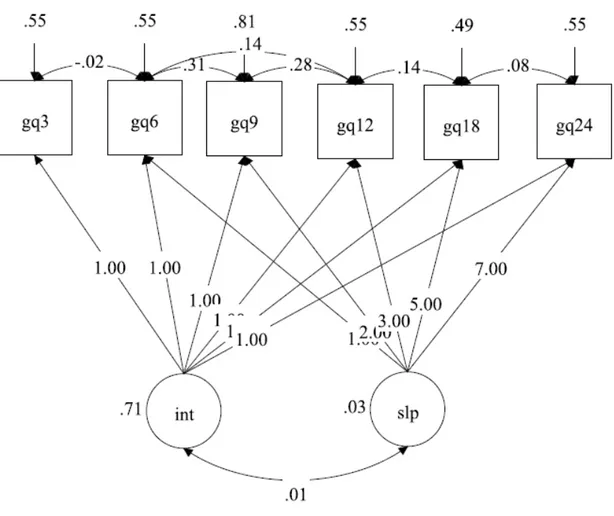
GQ-M1 – Unconditional linear curve model

The simplest LCM model estimated on the repeated measures of neurodevelopment is the unconditional linear model (Fig.15). The GQ-M1 model was defined with six repeated measures of GQ, from 3 to 24 months of age, assuming that observations were associated only with a latent intercept (labelled int) and a latent slope (slp). The linearity of the model was obtained by setting the loadings from the slope to the observed measures to values proportional to the time interval among measures (time unit is 3 months). Covariances on adjacent repeated measures were taken into account; the variances of GQ9 and of GQ18 were freely estimated to resolve a non-definite positive covariance matrix issue; the intercepts of GQ6 and GQ24 were freely estimated to obtain a better fit.

(40)

40

Figure 15 –Diagram of GQ-M1 model

Model GQ-M1 had a fair fit (RMSEA=0.077; CFI=0.984; TLI=0.979), indicating that a linear model is barely sufficient to explain the neurodevelopment pattern of growth. It gave estimates of the intercept (11.333) and of the slope (-0.386) means both significant at p<0.001, as well as the estimates of their variances; the covariance among the intercept and the slope was not significant (r=-0.075; p=0.504). Explained variance of each of the observed measures was very high, ranging from 0.516 for GQ9 to 0.801 for GQ24.

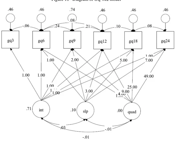
GQ-M2 – Unconditional quadratic curve model

The individual observed trajectories represented in Fig.13 and Fig.14 show that both standardized and raw neurodevelopment scores follow a curvilinear pattern; therefore, the first improvement on GQ-M1 model may be obtained by changing the curve pattern from linear to quadratic. In GQ-M2 model the quadratic term was named

(41)

41

quad; the intercepts of the observed measures at 6 and 18 months were freely estimated to obtain a better fit and

GQ18 variance was allowed to be freely estimated in order to resolve a non-positive definite covariance matrix issue.

The fit of the GQ-M2 Model (Fig.16) only slightly improved over the GQ-M1 Model, thus remaining at only a sufficient level (RMSEA=0.072, CFI=0.990, TLI=0.982). The quadratic latent variable had a significant mean (0.021, p<0.001), a non-significant variance (ψγ=0.001, p=0.088), was significantly associated with the slope (r=-0.860, p<0.001) and had no relation with the intercept (r=-0.201, p=0.476). The R2 of repeated measures increased, from a minimum of 0.591 for GQ9 to 0.812 for GQ24.

(42)

42

GQ-M3 – Unconditional completely latent trajectory model

The unsatisfactory fit of models GQ-M1 and GQ-M2 indicates that the trajectory of neurodevelopment may be neither linear or quadratic. In fact it may be seen from Fig.14 and from the series of GQ means in Tab.1 that decrease in time of GQ was not constant but occurred especially among 3 and 6 months and among 9 and 18 months; two periods of stability among 6 and 9 months and among 18 and 24 months concurred to define a quite irregular trajectory. Starting from this evidence, a completely latent trajectory model was designed in order to find out a trajectory of GQ where the shape of the longitudinal trend was estimated instead of being specified a priori. The loading from the latent slope to GQ3 was set to 0 and the loading to GQ6 was set to 1 in order to set the metric of change and all the other time points had free loadings. As a consequence, the estimated loadings were interpreted as the amount of change from GQ3 to each time point, scaled relative to the change that was observed between the first two periods. GQ9 and GQ18 variances were freely estimated to resolve non-positive definite covariance matrix issues.

(43)

43

Figure 17 –Diagram of GQ-M3 model

The GQ-M3 model had a much better fit compared to the previous models: RMSEA was 0.038 (90% C.I.: 0.000–0.078), CFI=0.997 and TLI=0.995. The estimated loadings reflected the pattern of change of GQ expressed by the series of means: λ9=1.12 indicated a change of GQ from 3 to 9 months only 12% higher than the change from 3 to 6 months; λ12 was 1.90, indicating a faster change from 9 to 12 months with respect to the previous 3 months; λ18 was 3.27 and λ24 was 3.28 indicating that a great change happened from 12 to 18 months while from 18 to 24 there was substantially no change in GQ. On the whole period from 3 to 18 months GQ changed 3.27 times as much as from 3 to 6 months. Since the mean of the slope estimate was negative (-0.587; p<0.001), higher loadings represent a greater decline of GQ with respect to the reference interval 3-6 months and positive differences among pairs of time points indicate a decline of GQ in corresponding interval: from 9 to 12 months the difference between loadings was 1.90-1.12=0.78, that is in those 3 months GQ declined at a pace that

(44)

44

equalled 78% of that observed among 3 and 6 months. From 18 to 24 months, the difference of 0.01 indicated that GQ scores estimates at 18 and at 24 months were unchanged. The intercept had a mean of 11.297 (corresponding to a GQ score of 112.97) and the correlation among intercept and slope was not significant, showing that at the individual level there was no association between the starting point of GQ and the rate of change. Variances of intercept and slope were both significant, representing high individual variations in starting points and in slopes. Significant correlations were found among each pair of adjacent periods except for the two initial and final intervals; the correlation among GQ6 and GQ12 was found significant and added to the model. Explained variances of the observed values were all quite or very high, ranging from 0.493 to 0.948.

The main characteristics of the first 3 models on neurodevelopment are summarized in Tab.3. Among these unconditional models, the Completely latent (GQ-M3) model was undoubtedly the best fitting because it had the best values on each of the five fit indices. For this reason it was taken as the basis model upon which add covariates to test the effects of clinical and socio-economic characteristics of the preterms on their neurodevelopment trajectories.

Tab.3 Main characteristics of Unconditional linear models on repeated measures of neurodevelopment

LCM UNCONDITIONAL MODELS GQ-M1 Linear GQ-M2 Quadratic GQ-M3 Completely latent Model fit RMSEA 0.077 0.072 0.038

CFI 0.984 0.990 0.997 TLI 0.979 0.982 0.995 AIC 4916.791 4911.125 4900.783 BIC 4977.283 4982.959 4968.837 Means Intercept 11.333 (p<0.001) 11.317 (p<0.001) 11.297 (p<0.001) Slope -0.386 (p<0.001) -0.426 (p<0.001) -0.587 (p<0.001) Variances Intercept 0.710 (p<0.001) 0.710 (p<0.001) 0.622 (p<0.001) Slope 0.027 (p<0.001) 0.104 (p=0.009) 0.123 (p<0.001) Correlation Intercept-slope 0.075 (p=0.504) 0.102 (p=0.657) 0.029 (p=0.787)

(45)

45

The complete description of GQ-M3 Model statistics are reported in Tab 4:

Tab 4 Parameter estimates, asymptotic standard errors and p-values of unconditional completely latent model for neurodevelopment (GQ-M3 Model), n=324

Parameter Estimate Standard Error p-value

Loadings λ0 0 λ1 1 λ2 1.115 0.079 <0.001 λ3 1.898 0.144 <0.001 λ4 3.270 0.299 <0.001 λ5 3.282 0.299 <0.001 Variances ψαα 0.622 0.140 <0.001 ψβ1β1 0.123 0.027 <0.001 Covariance ψαβ1 0.008 0.029 0.784 Means μα 11.297 0.059 <0.001 μβ -0.587 0.063 <0.001 Residual variances VAR(ε0) 0.577 0.042 <0.001 VAR(ε1) 0.577 0.042 <0.001 VAR(ε2) 0.815 0.078 <0.001 VAR(ε3) 0.577 0.042 <0.001 VAR(ε4) 0.109 0.107 0.308 VAR(ε5) 0.577 0.042 <0.001 Fit Statistics RMSEA 0.038 0.641a CFI 0.997 TLI 0.995 AIC 4900.783 BIC 4968.837

Number of free parameters (q) 18

N/q ratio 18.0

Estimated power 0.62

a

Probability for RMSEA ≤0.05

GQ-M4 – Conditional completely latent trajectory model with time-invariant covariates

The GQ-M4 model was built upon the GQ-M3 model by adding some time-invariant covariates. In this way, the GQ-M4 model retained the completely latent trajectory that proved to be the best fitting and added some

(46)

46

predictors that were associated with the latent intercept and/or slope. The time-invariant predictors to use in the model included ten of the variables described in the Materials and methods Section that on a clinical basis may be associated with the preterms’ neurodevelopment trajectory: Gender, Gestational age, SGA, Length of stay in the NICU, Mother’s age at birth, Twins, Migrant mother’s condition, Hollingshead Index, Diet at discharge and Sustained human milk feeding until 3 months of age. All continuous variables (Gestational age, Length of stay, Mother’s age and Hollingshead Index) were centered on their medians to obtain an estimated intercept that could be easily interpretable. Length of stay was expressed in months, by dividing the original variable by 30, and Hollingshead Index was divided by 10 to avoid the ill-scaled covariance matrix issue. As a first step, ten different models with each of these predictors as the only time-invariant covariate of latent intercept and slope were evaluated; each predictor proved to be significant on at least one of the two latent variables at p<0.200. Therefore, GQ-M4 Model was built including all predictors and removing one at a time, in decreasing order of p-value, those that were not significant at p<0.05 with each of the two latent variables. Starting from the complete model, SGA, Twins, Diet at discharge, Mothers’s age at birth, Gender and Gestational age were removed in sequence and hospital stay, Hollingshead Index, Migrant mother and Sustained milk were retained. The final GQ-M4 Model, where each time-invariant covariate is significant at p<0.05 on the intercept and/or the slope, is shown in Fig. 18.

(47)

47

Figure 18 –Diagram of GQ-M4 model (only significant paths are shown)

Model fit was very good: RMSEA was 0.022, with p(RMSEA≤0.05=0.927), CFI=0.997 and TLI=0.995; the comparative AIC and BIC indexes were sensibly lower than those found in GQ-M3 model. The excellent fit is also shown in Figure 19, where the two lines connecting the estimated and observed means perfectly overlap.