Applying Psychology of Persuasion to Conversational Agents
through Reinforcement Learning: an Exploratory Study
Francesca Di Massimo1, Valentina Carfora2, Patrizia Catellani2 and Marco Piastra1
1Computer Vision and Multimedia Lab, Università degli Studi di Pavia, Italy 2Dipartimento di Psicologia, Università Cattolica di Milano, Italy
[email protected] [email protected]
[email protected] [email protected]
Abstract
This study is set in the framework of task-oriented conversational agents in which dialogue managementis obtained via Re-inforcement Learning. The aim is to ex-plore the possibility to overcome the typ-ical end-to-end training approach through the integration of a quantitative model de-veloped in the field of persuasion psychol-ogy. Such integration is expected to accel-erate the training phase and improve the quality of the dialogue obtained. In this way, the resulting agent would take advan-tage of some subtle psychological aspects of the interaction that would be difficult to elicit via end-to-end training. We propose a theoretical architecture in which the psy-chological model above is translated into a probabilistic predictor and then integrated in the reinforcement learning process, in-tended in its partially observable variant. The experimental validation of the archi-tecture proposed is currently ongoing.
1 Introduction
A typical conversational agent has a multi-stage architecture: spoken language, written language and dialogue management, see Allen et al. (2001). This study focuses on dialogue management for task-oriented conversational agents. In particular, we focus on the creation of a dialogue manager aimed at inducing healthier nutritional habits in the interactant.
Given that the task considered involves psy-chosocial aspects that are difficult to program di-rectly, the idea of achieving an effective dialogue
Copyright c 2019 for this paper by its authors. Use per-mitted under Creative Commons License Attribution 4.0 In-ternational (CC BY 4.0).
manager via machine learning techniques, rein-forcement learning (RL) in particular, may seem attractive. At present, many RL-based approaches involve training an agent end-to-end from a dataset of recorded dialogues, see for instance Liu (2018). However, the chance of obtaining significant re-sults in this way entails substantial efforts in both collecting sample data and performing experi-ments. Worse yet, such efforts ought to rely on the even stronger hypothesis that the RL agent would be able to elicit psychosocial aspects on its own. As an alternative, in this study we envisage the possibility to enhance the RL process by harness-ing a model developed and accepted in the field of social psychology to provide a more reliable learning ground and a substantial accelerator for the process itself.
Our study relies on a quantitative, causal model of human behavior being studied in the field of so-cial psychology (see Carfora et al., 2019) aimed at assessing the effectiveness of message framing to induce healthier nutritional habits. The goal of the model is to assess whether messages with different frames can be differentially persuasive according to the users’ psychosocial characteristics.
2 Psychological model: Structural Equation Model
Three relevant psychosocial antecedents of be-haviour change are the following: Self-Efficacy (the individual perception of being able to eat healthy), Attitude (the individual evaluation of the pros and cons) and Intention Change (the indi-vidual willingness of adhering to a healthy diet). These psychosocial dimensions cannot be directly observed and need to be measured as latent vari-ables. To this purpose, questionnaires are used, each composed by a set of questions or items (i.e. observed variables). Self-Efficacy is mea-sured with 8 items, each associated to a set of answers ranging from "not at all confident" (1)
Figure 1: SEM simplified model for the case at hand.
Figure 2: DBN translation of the SEM shown in Figure 1.
to "extremely confident" (7). Attitude is assessed through 8 items associated to a differential scale ranging from 1 to 7 (the higher the score, the more positive the attitude). Intention Change is mea-sured with three items on a Likert scale, ranging from 1 (“definitely do not”) to 7 (“definitely do”). See Carfora et el. (2019).
In our study, the psychosocial model was as-sessed experimentally on a group of volunteers. Each participant was first proposed a question-naire (Time 1 – T1) for measuring Self-Efficacy, Attitude and Intention Change. In a subsequent phase (i.e. message intervention), participants were randomly assigned to one of four groups, each receiving a different type of persuasive mes-sage: gain (i.e. positive behavior leads to posi-tive outcomes), non-gain (negaposi-tive behavior pre-vents positive outcomes), loss (negative behavior leads to negative outcomes) and non-loss (posi-tive behavior prevents nega(posi-tive outcomes) (Hig-gins, 1997; Cesario et al., 2013). In a last phase (Time 2 - T2), the effectiveness of the message in-tervention was then evaluated with a second ques-tionnaire, to detect changes in participants’
Atti-tude and Intention Change in relation to healthy eating.
The overall model is described by the Struc-tural Equation Model (SEM, see Wright, 1921) in Figure 1. For simplicity, only three items are shown for each latent variable. Besides allow-ing the description of latent variables, SEMs are causalmodels in the sense that they allow a sta-tistical analysis of the strength of causal relations among the latents themselves, as represented by the arrows in figure. SEMs are linear models, and thus all causal relations underpin linear equations. Note that latent variables in a SEM have dif-ferent roles: in this case gain/non-gain/loss/non-lossmessages are independent variables, Intention Changeis a dependent variable, Attitude is a me-diatorof the relationship between the independent and the dependent variables, and Self-Efficacy is a moderator, namely, it explains the intensity ot the relation it points at. Intention Change was mea-sures at both T1 and T2, Attitude was measured at both T1 and T2, and Self-Efficacy was measured at T1 only. Note that the time transversality (i.e. T1 → T2) is implicit in the SEM depiction above.
3 Probabilistic model: Bayesian Network
Once the SEM is defined, we aim to translate it into a probabilistic model, so as to obtain the probability distributions needed for the learning process. We resort to a graphical model, and in particular to a Bayesian Network (BN, see Ben Gal, 2007), namely a graph-based description of both the observable and latent random variables in the model and their conditional dependencies. In BNs, nodes represent the variables and edges rep-resent dependencies between them, whereas the lack of edges implies their independence, hence a simplification in the model. As a general rule, the joint probability of a BN can be inferred as follows: P (X1, . . . , XN) = N Y i=1 P (Xi| parents(Xi)),
where X1, . . . , XN are the random variables in
the model and parents(Xi) indicate all the nodes
having an edge oriented towards Xi.
In the case at hand, a temporal description of the model, accounting for the time steps T1 and T2, is necessary as well. For this purpose, we use a Dynamic Bayesian Network (DBN, see Dagum et al., 1992). The DBN thus obtained is shown in Figure 2.
Notice that the messages are only significant at T2, as they have not been sent yet at T1. We gath-ered message in the one node Message Type, as-suming it can take four, mutually exclusive values. The mediator Attitude is measured at both time steps while the moderator Self-Efficacy is constant over time, as suggested in Section 2. Intention Changehas relevance at T2 only since, as we will mention in Section 5, it will be used to estimate a reward function once the final time step is reached.
4 Learning the BN
The collected data are as follows. The analysis was conducted on 442 interactants, divided in four groups, each one receiving a different type of mes-sages1. The answers to the items of the ques-tionnaire always had a range of 7 values. How-ever, this induces a combinatory esplosion, mak-ing it impossible to cover all the subspaces (78 = 5.764.801 different combinations for Attitude, for instance). We thus decide to aggregate: low :=
1The original study included also a control group, which
we do not consider here.
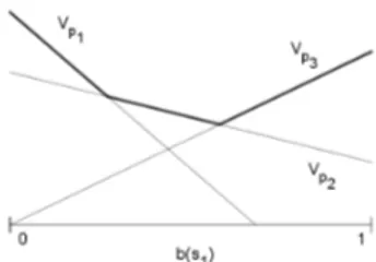
Figure 3: Basic example of computation of Vπ in
a case where S = {s1, s2}. p1, p2, p3 are three
possible policies.
(1 to 2); medium := (3 to 5); high := (6 to 7). Our aim is to learn the Joint Probability Distri-bution(JPD) of our model, as that would make us able to answer, through marginalizations and con-ditional probabilities, any query about the model itself. The conditional probability distributions to be learnt in the case in point are then the follow-ing:
• P (Item Ai), for i = 1, . . . , 8; • P (Item SEi), for i = 1, . . . , 8; • P (Message Type);
• P (Attitude T 1 | Item Ai, i = 1, . . . , 8); • P (Self-Efficacy | Item SEi, i = 1, . . . , 8); • P (Attitude T 2 | Item Ai, i = 1, . . . , 8,
Message Type, Self-Efficacy); • P (Intention Change | Attitude T 2,
Self-Efficacy).
The first three can be easily inferred from the raw data as relative frequencies. As for the following four, even aggregating the 7 values as mentioned, a huge amount of data would still be necessary (38·24·3 = 314.928 subspaces for Attitude T2, for
instance). As conducting a psychological study on that amount of people would not be feasible, we address the issue with an appropriate choice of the method. To allow using Maximum Likelihood Es-timation(MLE) to learn the BN, we resort to the Noisy-ORapproximation (see Oni´sko, 2001). Ac-cording to this, through a few appropriate changes (not shown) to the graphical model, the number of subspaces can be greatly reduced (e.g. 3·2·3 = 18 for Attitude T2).
5 Reinforcement Learning: Markov Decision Problems
The translation into a tool to be used for reinforce-ment learning is obtained in the terms of Markov
Decision Processes (MDPs), see Fabiani et al. (2010).
Roughly speaking, in a MDP there is a finite number of situations or states of the environment, at each of which the agent is supposed to select an action to take, thus inducing a state transition and obtaining a reward. The objective is to find a pol-icydetermining the sequence of actions that gen-erates the maximum possible cumulative reward, over time. However, due to the presence of latents, in our case the agent is not able to have complete knowledge about the state of the environment. In such a situation, the agent must build its own esti-mate about the current state based on the memory of past actions and observations. This entails using a variant of the MDPs, that is Partially Observable Markov Decision Processes(POMDPs, see Kael-bling 1998). We then define the following, with reference to the variables mentioned in Figure 2:
S := {states} = {Attitude T 2, Self-Efficacy}; A := {actions} = {ask A1, . . . , ask A8} ∪ {ask SE1, . . . , ask SE8} ∪ {G, N G, L, N L}, where Ai denotes the question for Item Ai, SEi denotes the question for Item SEi and G, N G, L, N L denote the action of sending Gain, Non-gain, Loss and Non-loss messages respec-tively;
Ω := {observations} =
{Item A1, . . . , Item A8, Item SE1, . . . , Item SE8}. Starting from an unknown initial state s0(often
taken to be uniform over S, as no information is available), the agent takes an action a0, that brings
it, at time step 1, to state s1, unknown as well.
There, an observation o1is made.
The process is then repeated over time, until a goalstate of some kind has been reached. Hence, we can define the history as an ordered succession of actions and observations:
ht:= {a0, o1, . . . , at−1, ot} , h0 = ∅.
As at all steps there is uncertainty about the ac-tual state, a crucial role is played by the agent’s estimate about the state of the environment, i.e. by the belief state. The agent’s belief at time step t, denoted as bt, is driven by its previous belief bt−1
and by the new information acquired, i.e. the ac-tion taken at−1and observation made ot. We then
have:
bt+1(st+1) = P (st+1| bt, at, ot+1).
In the POMDP framework, the agent’s choices about how to behave are influenced by its belief state and by the history. Thus, we define the agent’s policy:
π = π(bt, ht),
that we aim to optimize. To complete the picture, we define the following functions to describe the model evolution in time (the notation0 indicates a reference to the subsequent time step):
state-transition function: T : (s, a) 7→ P (s0 | s, a) := T (s0, s, a); observation function: O : (s, a) 7→ P (o0 | a, s0) := O(o0, a, s0); reward function: R : (s, a) 7→ E [r0 | s, a] := R(s, a). These functions can be easily adapted to the specifics of the case at hand. It can be seen that, once the JPD derived from the DBN is completely specified, the reward is deterministic. In particu-lar, it is computed by evaluating the changes in the values for the latent Intention Change.
As we are interested in finding an optimal pol-icy, we now need to evaluate the goodness of each state when following a given policy. As there is no certainty about the states, we define the value functionas a weighted average over the possible belief states:
Vπ(bt, ht) :=
X
st
bt(st)Vπ(st, bt, ht),
where Vπ(st, bt, ht) is the state value function.
The latter depends on the expected reward (and on a discount factor γ ∈ [0, 1] stating the preference for fast solutions):
Vπ(st, bt, ht) :=R(st, π(bt, ht)) + γX st+1 T (st+1,st, π(bt, ht)) ∗ X ot+1 O(ot+1, π(bt, ht),st+1)Vπ(st+1, bt+1, ht+1).
Finally, we define the target of our seek, namely the optimal value function and the related optimal policy, as:
(
V∗(bt, ht) := maxπVπ(bt, ht),
π∗(bt, ht) := argmaxπVπ(bt, ht).
It can be shown that the optimal value function in a POMDP is always piecewise linear and convex, as
Figure 4: Expansion of the policy tree. l, m, h stand for low, medium and high.
exemplified in Figure 3. In other words, the opti-mal policy (in bold in Figure 3) combines different policies depending on their belief state values.
The next step is to use the POMDP to detect the optimal policy, that is the sequence of questions to ask to the interactant, in order to draw her/his pro-file, hence the message to send, which maximizes the effectiveness of the interaction. To this end, the contribution of the DBN is fundamental. From the JPD associated, in fact, we construct the probabil-ity distributions necessary to define the functions T , O, R that compose the value function.
6 Policy from Monte Carlo Tree Search
It is evident from Figure 4, describing the full ex-pansion of the policy tree for the case in point, that the computational effort and power required for a brute-force exploration of all possible com-binations is unaffordable.
Among all the policies that can be considered, we want to select the optimal ones, thus avoid-ing coinsideravoid-ing policies that are always underper-forming. In other words, with reference to Fig-ure 3, we want to find Vp1, Vp2, Vp3 among those
of all possible policies, and use them to identify the optimal policy V∗.
To accomplish this, we select the Monte Carlo Tree Search(MCTS) approach, see Chaslot et al. (2008), due to its reliability and its applicability to computationally complex practical problems. We adopt the variant including an Upper Confidence Bound formula, see Kocsis et al. (2006). This method combines exploitation of the previously computed results, allowing to select the game ac-tion leading to better results, with exploraac-tion of different choices, to cope with the uncertainty of the evaluation. Thus, using Vπ(st, bt, ht) as
de-fined before to guide the exploration, the MCTS method reliably converges (in probability) to
op-timal policies. These latter will be applied by the conversational agent in the interaction with each specific user, to adapt both the sequence and the amount of questions to her/his personality profile and selecting the message which is most likely to be effective.
7 Conclusions and future work
In this work we explored the possibility of har-nessing a complete and experimentally assessed SEM, developed in the field of persuasion psy-chology, as the basis for the reinforcement learn-ing of a dialogue manager that drives a conversa-tional agent whose task is inducing healthier nu-tritional habits in the interactant. The fundamen-tal component of the method proposed is a DBN, which is derived from the SEM above and acts like a predictor for the belief state value in a POMDP.
The main expected advantage is that, by doing so, the RL agent will not need a time-consuming period of training, possibly requiring the involve-ment of human interactants, but can be trained ‘in house’ – at least at the beginning – and be released in production at a later stage, once a first effec-tive strategy has been achieved through the DBN. Such method still requires an experimental valida-tion, which is the current objective of our working group.
Acknowledgments
The authors are grateful to Cristiano Chesi of IUSS Pavia for his revision of an earlier version of the paper and his precious remarks. We also acknowledge the fundamental help given by Re-becca Rastelli, during her collaboration to this re-search.
References
Allen, J., Ferguson, G., & Stent, A. 2001. An archi-tecture for more realistic conversational systems. In Proceedings of the 6th international conference on Intelligent user interfaces (pp. 1-8). ACM.
Anderson, Ronald D. & Vastag, Gyula. 2004. Causal modeling alternatives in operations re-search: Overview and application. European Jour-nal of OperatioJour-nal Research. 156. 92-109.
Auer, Peter & Cesa-Bianchi, Nicolò & Fischer, Paul. 2002Kocsis, Levente & Szepesvári, Csaba. 2006. Bandit Based Monte-Carlo Planning. Finite-time Analysis of the Multiarmed Bandit Problem. Ma-chine Learning. 47. 235-256.
Bandura, A. 1982. Self-efficacy mechanism in human agency. American Psychologist, 37, 122-147. Baron, Robert A. & Byrne, Donn Erwin & Suls, Jerry
M. 1989. Exploring social psychology, 3rd ed. Boston, Mass.: Allyn and Bacon. 0205119085. Ben Gal I. 2007. Bayesian Networks. Encyclopedia of
Statistics in Quality and Reliability. John Wiley & Sons.
Bertolotti, M., Carfora, V., & Catellani, P. 2019. Dif-ferent frames to reduce red meat intake: The moder-ating role of self-efficacy. Health Communication, in press.
Carfora, V., Bertolotti, M., & Catellani, P. 2019. In-formational and emotional daily messages to reduce red and processed meat consumption. Appetite, 141, 104331.
Cesario, J., Corker, K. S., & Jelinek, S. 2013. A self-regulatory framework for message framing. Journal of Experimental Social Psychology, 49, 238-249. Chaslot, Guillaume & Bakkes, Sander & Szita, Istvan
& Spronck, Pieter. 2008. Monte-Carlo Tree Search: A New Framework for Game AI. Bijdragen. Dagum, Paul and Galper, Adam and Horvitz, Eric.
1992. Dynamic Network Models for Forecasting. Proceedings of the Eighth Conference on Uncer-tainty in Artificial Intelligence.
Dagum, Paul and Galper, Adam and Horvitz, Eric and Seiver, Adam. 1999. Uncertain reasoning and fore-casting. International Journal of Forefore-casting. De Waal, Alta & Yoo, Keunyoung. 2018. Latent
Vari-able Bayesian Networks Constructed Using Struc-tural Equation Modelling. 2018 21st International Conference on Information Fusion. 688-695. Fabiani, Patrick & Teichteil-Königsbuch, Florent.
2010. Markov Decision Processes in Artificial In-telligence. Wiley-ISTE.
Gupta, Sumeet & W. Kim, Hee. 2008. Linking structural equation modeling to Bayesian networks: Decision support for customer retention in virtual communities. European Journal of Operational Re-search. 190. 818-833.
Heckerman, David. 1995. A Bayesian Approach to Learning Causal Networks.
Higgins, E.T. 1997. Beyond pleasure and pain. Amer-ican Psychologist, 52, 1280-1300.
A. Howard, Ronald. 1972. Dynamic Programming and Markov Process. The Mathematical Gazette. 46.
Pack Kaelbling, Leslie & Littman, Michael & R. Cas-sandra, Anthony. 1998. Planning and Acting in Par-tially Observable Stochastic Domains. Artificial In-telligence. 101. 99-134.
Kocsis, Levente & Szepesvári, Csaba. 2006. Bandit Based Monte-Carlo Planning. Machine Learning: ECML 2006. Springer Berlin Heidelberg. 282-293. Lai, T.L & Robbins, Herbert. 1985. Asymptotically
Ef-ficient Adaptive Allocation Rules. Advances in Ap-plied Mathematics. 6. 4-22.
Liu, Bing. 2018. Learning Task-Oriented Dialog with Neural Network Methods. PhD thesis.
Murphy, Kevin. 2012. Machine Learning: A Proba-bilistic Perspective. The MIT Press. 58.
Pearl Judea. 1988. Probabilistic Reasoning in In-telligent Systems: Networks of Plausible Inference. Representation and Reasoning Series (2nd printing ed.). San Francisco, California: Morgan Kaufmann. Oni´sko, Agnieszka & Druzdzel, Marek J. & Wasyluk, Hanna. 2001. Learning Bayesian network parame-ters from small data sets: application of Noisy-OR gates. International Journal of Approximate Rea-soning. 27.
Silver, David & Veness, Joel. 2010. Monte-Carlo Planning in Large POMDPs. Advances in Neural Information Processing Systems. 23. 2164-2172. Matthijs T. J. Spaan. 2012. Partially Observable
Markov Decision Processes. In: Reinforcement Learning: State of the Art. Springer Verlag. 387-414.
Sutton, Richard & G. Barto, Andrew. 1998. Reinforce-ment Learning: An Introduction. IEEE transactions on neural networks / a publication of the IEEE Neu-ral Networks Council. 9. 1054.
Wright, Sewall. 1921. Correlation and causation. Journal of Agricultural Research. 20. 557–585. Young, Steve & Gasic, Milica & Thomson, Blaise &
Williams, Jason. 2013. POMDP-based statistical spoken dialog systems: A review. Proceedings of the IEEE, 101. 1160-1179.