DOTTORATO DI RICERCA IN
INGEGNERIA CIVILE, AMBIENTALE E DEI MATERIALI
Ciclo XXIXSettore Concorsuale di afferenza: 08/A1 Settore Scientifico disciplinare: ICAR/02
TITOLO TESI
AN INTEGRATED DECISION SUPPORT SYSTEM FOR THE
PLANNING, ANALYSIS, MANAGEMENT AND REHABILITATION OF
PRESSURISED IRRIGATION DISTRIBUTION SYSTEMS
Presentata da: Abdelouahid Fouial
Coordinatore Dottorato: Prof. Luca Vittuari
Relatore: Prof. Armando Brath
i
Water scarcity is a mounting problem in arid and semi-arid regions such as the Mediterranean. Therefore, smarter and more effective water management is required, especially in irrigated agriculture. Irrigation infrastructure such as pressurized irrigation distribution systems (PIDSs) play an important role for the intensification of agricultural production in the Mediterranean region. However, the operation and management of these systems can be complex as they involve several intertwined processes, which need to be considered simultaneously. For this reason, numerous decision support systems (DSSs) have been developed and are available to deal with these processes, but as independent components.
To this end, a comprehensive DSS called DESIDS has been developed and tested in the framework of this research. This DSS has been developed bearing in mind the need of irrigation district managers for an integrated tool that can assist them in taking strategic decisions for managing and developing reliable, adequate and sustainable water distribution plans, which provide the best services to farmers. Hence, four modules were integrated in DESIDS: i) the irrigation demand and scheduling module; ii) the hydraulic analysis module; iii) the operation and management modules; and iv) the design and rehabilitation module.
DESIDS was tested on different case studies located in the Apulia region (Southern Italy), where it proved to be a valuable tool for irrigation district managers as it provides a wide range of decision options for proper operation and management of PIDSs. All this is obtained through a DSS that offers: i) high level of interactivity and ease of use; ii) complete control of the irrigation managers; iii) adaptability and flexibility to the problems related to the operation of PIDSs; and iv) effectiveness in assisting irrigation managers with the decision making process. The developed DSS can be used as a platform for future integrations and expansions to include other processes needed for better decision-making support.
ii
I dedicate this thesis to
My parents, my sisters and brothers
iii
First and foremost I wish to thank my advisor, Professor Armando Brath, for his support and guidance during my PhD research. Beside my advisor, I would like to thank Professor Cristiana Bragalli and Dr. Alessio Domeneghetti for their insightful comments and encouragement, and for providing me with the tools that I needed to choose the right direction and successfully complete my thesis.
I would also like to express my special appreciation and thanks to Professor Nicola Lamaddalena, Head of the Land and Water Resources Department at IAM Bari, for being a tremendous mentor for me. His guidance and encouragement allowed me to grow as a researcher. His advice on both research as well as on my career have been priceless. This PhD research would not have been possible without his help and the financial support of IAM Bari. I greatly appreciate the support received through the collaborative work undertaken with the University of Cordoba, Spain. My sincere thanks go to Professor Juan A. Rodríguez Díaz for his brilliant comments and suggestions. Thanks also to the members of his team at the Department of Agronomy for their support and friendship.
I am very grateful to Dr. Fadhila Lahmer who was always so helpful and provided me with valuable advice. I also thank all the staff of IAM Bari for their support and kindness.
A special thanks to my family for all their love and encouragement. Words cannot express how grateful I am to my parents for all the sacrifices they have made on my behalf. Finally, I would like to thank all my friends who supported me, and motivated me to strive towards my goal.
Abdelouahid Fouial Bari, February 12, 2017
iv
Abstract ... i
Acknowledgements ... iii
Table of Contents ... iv
List of Figures ... viii
List of Tables ...x
Abbreviations &Notation ... xi
CHAPTER I ...1
Introduction I.1 Background and Motivation ... 1
I.2 Aims and objectives ... 6
I.3 Outline of the thesis ... 6
I.4 References ... 8
CHAPTER II...10
DESIDS: Decision Support for Irrigation Distribution Systems II.1 Introduction ... 10
II.2 DSS description ... 13
II.3 Irrigation demand and scheduling module ... 15
II.3.1 Irrigation Requirements ... 15
II.3.2 Irrigation scheduling ... 17
II.3.3 Generation of open hydrants configurations ... 18
II.4 Hydraulic analysis module ... 19
II.4.1 Demand-Driven Analysis ... 19
II.4.2 Pressure-Driven Analysis ... 20
II.4.3 Performance indicators ... 22
II.4.4 Assessment of the hydraulic performance ... 24
II.5 Operation and management module ... 26
II.5.1 Genetic Algorithms ... 27
II.5.2 Optimization of irrigation periods ... 28
II.6 Design and rehabilitation module ... 29
v
II.8 References ... 33
CHAPTER III ...38
Generating Hydrants’ Configurations for Efficient Analysis and Management of Pressurized Irrigation Distribution Systems III.1 Introduction ... 38
III.2 Methodology ... 41
III.2.1 Crop water requirements and irrigation scheduling ... 41
III.2.2 Generation of hydrants opening configurations ... 42
III.2.3 Hydraulic Analysis ... 43
III.2.4 Case study ... 43
III.3 Results and discussions ... 44
III.3.1 Estimation of irrigation scheduling ... 45
III.3.2 Generation of hydrants configurations ... 46
III.3.3 Hydraulic analysis ... 48
III.4 Conclusion ... 51
III.5 References ... 52
CHAPTER IV ...54
Optimal Operation of Pressurised Irrigation Distribution Systems Operating by Gravity IV.1 Introduction ... 54
IV.2 Methodology ... 56
IV.2.1 Irrigation water requirements ... 56
IV.2.2 Hydraulic Analysis ... 57
IV.2.3 Irrigation periods optimization ... 58
IV.2.4 Performance assessment ... 59
IV.3 Case Study ... 59
IV.4 Results and discussions ... 61
IV.4.1 Water requirements ... 61
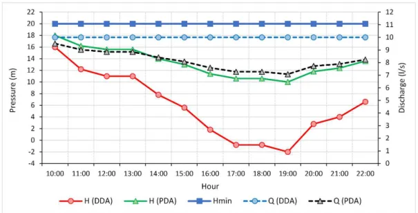
IV.4.2 Hydraulic Analysis for the current on-demand operating conditions ... 61
IV.4.3 Optimal management of the network ... 63
vi
CHAPTER V ...73
Multi-Objective Optimization Model based on Localized Loops for the Rehabilitation of Pressurized Irrigation Distribution Networks V.1 Introduction ... 73
V.2 Methodology ... 76
V.2.1 Case study ... 76
V.2.2 Step 1: Initial hydraulic analysis of the existing network ... 77
V.2.3 Step 2: Optimization of PIDN rehabilitation ... 78
V.2.3.1 Determination of looping positions ... 78
V.2.3.2 Objective functions ... 79
V.2.3.3 Optimization process ... 80
V.3 Results and discussions ... 82
V.3.1 Determination of the upstream discharge and piezometric elevation ... 82
V.3.2 Initial hydraulic Analysis of the existing network ... 83
V.3.3 Rehabilitation alternatives ... 84
V.4 Conclusions ... 90
V.5 References ... 93
CHAPTER VI ...96
Modelling the impact of climate change on pressurized irrigation distribution systems: Use of a new tool for adaptation strategy implementation VI.1 Introduction ... 96
VI.2 Study area ... 98
VI.3 Methodology ... 99
VI.3.1 Climate change scenarios ... 99
VI.3.2 Irrigation water requirements ... 100
VI.3.3 Hydraulic analysis ... 100
VI.3.4 Adaptation strategy ... 101
VI.4 Results and discussions ... 101
VI.4.1 Impact of climate change on ET0 and rainfall ... 101
VI.4.2 Performance of the distribution system ... 104
vii
CHAPTER VII ...114 General Conclusions
VII.1 Conclusions ... 114 VII.2 Published and presented works ... 117
viii
Fig. I-1. Projection of the intensity of water stress and scarcity ... 2
Fig. I-2 Diagram of the actions, effects, technical results and outputs related to irrigation modernization and optimization ... 5
Fig. II-1. Main interface of DESIDS ... 13
Fig. II-2. DESIDS integrated modules ... 14
Fig. II-3. Irrigation demand and scheduling module ... 16
Fig. II-4. Setting of the added devices for each open hydrant in the PDA ... 22
Fig. II-5. Hydraulic analysis module ... 25
Fig. II-6. Flowchart of the hydraulic analysis module ... 26
Fig. II-7. Optimization of irrigation periods ... 27
Fig. II-8. General flowchart of the operation and management module ... 29
Fig. II-9. The optimization module in DESIDS ... 32
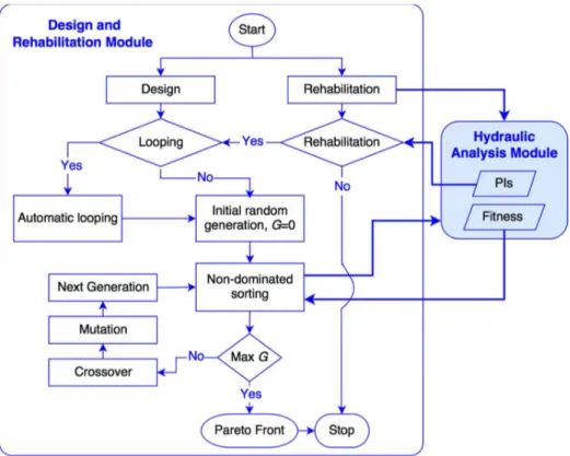
Fig. II-10. General flowchart for the design and rehabilitation module ... 33
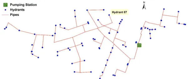
Fig. III-1. Layout of District 1-a system ... 44
Fig. III-2. Probability of hydrant opening time ... 45
Fig. III-3. Determination of the peak period ... 46
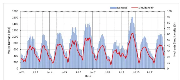
Fig. III-4. Water demand and hydrant simultaneity of the peak period ... 48
Fig. III-5. RPD indicator for DDA and PDA for the peak demand day ... 49
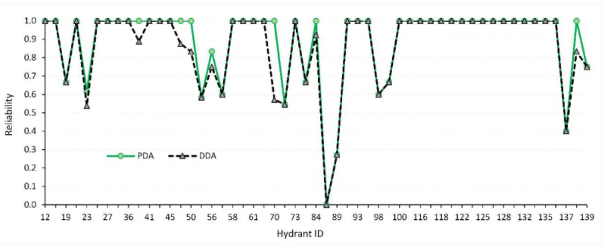
Fig. III-6. Reliability indicator for DDA and PDA for the peak day ... 49
Fig. III-7. Pressure and discharge at hydrant 87 resulted from DDA and PDA ... 50
Fig. III-8. ADF resulted from PDA of the peak demand day ... 51
Fig. IV-1. Optimization of irrigation periods using DESIDS ... 57
Fig. IV-2. Layout of District 4 irrigation distribution network ... 60
Fig. IV-3. RPD for the current operating conditions with an upstream discharge of 1200 ls-1 63 Fig. IV-4. Re for the current operating conditions with an upstream discharge of 1200 ls-1 ... 63
Fig. IV-5. RPD of the optimal solutions with an upstream discharge of 1200 ls-1... 64
Fig. IV-6. PE for each simulated configuration of open hydrants ... 65
Fig. IV-7. Pressure deficit for each individual in the last generation for the upstream discharge of 2000 ls-1 ... 66
Fig. IV-8. RPD for the current on-demand conditions and the optimal solution with an upstream discharge of 1650 ls-1 ... 67
ix
Fig. IV-10. Upstream discharges of District 4 after irrigation periods optimization ... 69
Fig. V-1. Layout of Sector 13 network ... 77
Fig. V-2. Flowchart for the optimization of rehabilitation ... 82
Fig. V-3. Frequency of flow and piezometric elevation at the intake of Sector 13 ... 83
Fig. V-4. RPD for the actual situation of Sector 13 network ... 84
Fig. V-5. Reliability for the actual situation of Sector 13 network ... 84
Fig. V-6. Pareto optimal solutions ... 85
Fig. V-7. RPD for the rehabilitated Sector 13 network (Case 1) ... 86
Fig. V-8. Reliability for the rehabilitated Sector 13 network (Case 1) ... 87
Fig. V-9. RPD for the rehabilitated Sector 13 network (Case 2) ... 87
Fig. V-10. Reliability for the rehabilitated Sector 13 network (Case 2) ... 88
Fig. V-11. RPD for the rehabilitated Sector 13 network (Case 3) ... 89
Fig. V-12. Reliability for the rehabilitated Sector 13 network (Case 3) ... 89
Fig. V-13. Pressure deficits and associated rehabilitation costs ... 90
Fig. VI-1. Flowchart summarizing various calculation steps within DESIDS ... 99
Fig. VI-2. Projected future changes (2050s and 2080s) in ET0, GIR and rainfall using RCP2.6 and RCP8.5 scenarios ... 102
Fig. VI-3. Current and future (2050s and 2080s) monthly ET0 and rainfall using RCP2.6 and RCP8.5 scenarios ... 103
Fig. VI-4. RPD envelope (90%) under current and future climate (2050s and 2080s) using RCP2.6 and RCP8.5 scenarios ... 105
Fig. VI-5. Location of the loops proposed to improve the current and future performance of District 4 network ... 106
Fig. VI-6. Current and future performance of District 4 with existing, redesigned and localized loop solutions as evaluated using RPD indicator ... 107
Fig. VI-7. Current and future performance of District 4 with existing, redesigned and localized loop solutions as evaluated using hydrants reliability indicator. ... 108
x
Table III-1. Crop allocation in District 1-a ... 44 Table IV-1. Crops allocation in District 4 ... 61 Table VI-1 System performance classified by RPD and hydrants Re indicators ... 101 Table VI-2. Specific continuous discharge and peak upstream discharge under present and future (2050's and 2080's) climate with RCP2.6 and RCP8.5 scenarios ... 104 Annex V-1. Pipe diameters in the existing network and the selected rehabilitation cases... 91 Annex VI-1. List of the GCMs used by MarkSim GCM® to project future climate ... 110
xi
ABBREVIATIONS
AR Assessment Report CV Check Valve
CWR Crop Water Requirement DDA Demand-Driven Analysis
DESIDS Decision Support for Irrigation Distribution Systems DSS Decision Support System
FCV Flow Control Valve GA Genetic Algorithm
GCMs Global Circulation Models GGA Global Gradient Algorithm
IPCC Intergovernmental Panel on Climate Change MOEAs Multi-Objective Evolutionary Algorithms NSGA II Non-dominated Sorting Genetic Algorithm II PDA Pressure-Driven Analysis
PI Performance Indicator
PIDN Pressurized Irrigation Distribution Network PIDS Pressurized Irrigation Distribution System RCPs Representative Concentration Pathways WDS Water Distribution System
NOTATION
Average pressure head in the best quarter m Average pressure head in the poorest quarter m
A Topological incidence Matrix -
A Area irrigated by a hydrant ha
ADF Available discharge fraction for a hydrant -
AVFnet Available Volume fraction for a network -
CR Capillary rise from the groundwater table mm
DP Deep percolation mm
Dr, Root zone depletion mm
ea Actual vapor pressure kPa
Eirr Irrigation efficiency %
xii
ETo Reference evapotranspiration mm
G Soil heat flux density MJ m-2
day-1
GIR Gross irrigation requirement mm
H Pressure head at a hydrant m
H Column vector of the computed nodal total heads - H0 Column vector of the known nodal total heads
Hmin Minimum required pressure head at a hydrants m
i Subscript for the day -
I Net irrigation depth on a specific day mm
Imax Maximum possible irrigation depth mm
j Subscript indicating hydrants -
k Subscript indicating pipes -
Kc Crop coefficient -
Ks Water stress coefficient -
l Subscript indicating loops -
n Exponent of the flow in the head loss equation - n0 Number of nodes with known pressure head (reservoirs)
Nconf Number of open hydrants configurations -
nd Subscript indicating nodes -
Nhyd Total number of open hydrants -
NIR Net irrigation requirement mm
nn Number nodes with unknown pressure heads -
No Total number of times where hydrant j is open -
np Number of pipes carrying unknown flows -
Np Number of irrigation periods -
Ns Number of times the pressure at a hydrant satisfied -
OFCR Objective function of minimization of total cost of rehabilitation - OFPD Objective function of pressure deficit minimization -
P Rainfall mm
PE Pressure Equity -
Peff Effective rainfall mm
Ppq Pressure Equity -
q Nominal discharge of a hydrant Ls-1
Q Column vector of the computed pipe flows -
xiii
Qup Upstream discharge at the head of the network ls-1
R Resistance factor for a pipe -
Ra Extraterrestrial radiation mm day-1
RAW Readily available water mm
Re Reliability -
Rn Net radiation at the crop surface MJ m
-2
day-1
RO Runoff from the soil surface mm
RPD Relative pressure deficit -
T Mean air temperature °C
TAW Total available water mm
th Operating time of hydrants h
tir Irrigation time h
Tmax Minimum air temperature °C
Tmin Maximum air temperature °C
u2 Wind speed at 2 m height m s-1
Vact Total volume of water actually supplied by a network m3
Vreq Total volume required to be supplied by a network m3
X, Y coordinates of nodes -
γ Psychrometric constant kPa °C-1
Δ Slope vapor pressure curve kPa°C-1
Nk Total number of pipes in a network -
L Length of a pipe m
D Pipe diameter mm
1
I
NTRODUCTIONI.1 Background and Motivation
Water scarcity is a mounting challenge that is affecting food security of large areas of the world. FAO (2012) defined water scarcity as a gap between available supply and expressed demand of freshwater in a specified domain, under prevailing institutional arrangements (including both resource ‘pricing’ and retail charging arrangements) and infrastructural conditions.
Physical water scarcity occurs when there are inadequate resources to satisfy demand. It is also important to consider the economic water scarcity, which is caused by a lack of investment in water to satisfy the demand. Most countries have enough water to meet domestic, agricultural, industrial and environmental requirements. In this case, the problem is in the management. Even though water scarcity is regarded as not having enough water to meet domestic needs, it is agriculture that will face the real challenge as it takes roughly 70 times more water to produce food than people use for domestic purposes (UNDP, 2006).
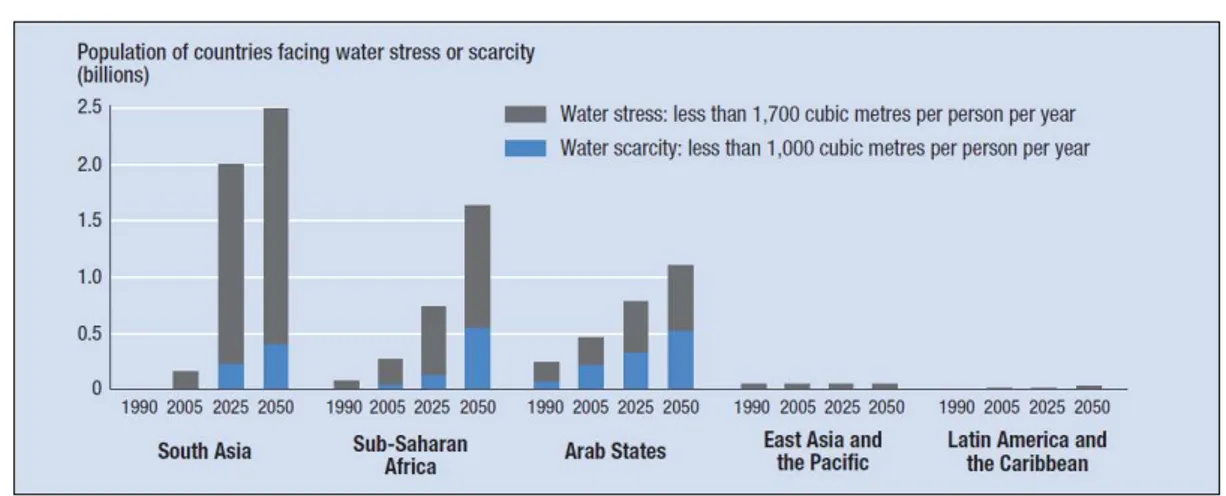
Food production plays a critical role in sustainable development and provides employment for 40% of the global population (UNEP, 2012). Furthermore, 70% of the world’s freshwater withdrawals are already committed to irrigated agriculture and that more water will be needed in order to meet increasing demands for food and energy (biofuels) (WWAP, 2012). This will eventually put a lot of pressure on the available finite water resources. By 2025, more than 3 billion people could be living in water-stressed countries, and 14 countries will slip from water stress to water scarcity as illustrated in Fig. I-1 (UNDP, 2006). In addition, water scarcity is expected to affect more than 1.8 billion people, hurting agricultural workers and poor farmers the most (UNDP, 2014)
2
Source: UNDP (2006)
Fig. I-1. Projection of the intensity of water stress and scarcity
To tackle this problem, smarter and more effective water management is required as it will be a major challenge to achieve the necessary boost in food production while maintaining an acceptable increase in water use. In other words, there will be needs to invest in modernization of infrastructure, to restructure institutions and to upgrade the technical capacities of water managers and farmers. Water use efficiency, producing more ‘crop per drop’, will be a major challenge (UNEP, 2012). This will eventually increase water productivity. Molden (2007) stated that, under optimistic assumptions about water productivity gains, three-quarters of the additional food demand can be met by improving water productivity on existing irrigated lands. The term ‘efficiency’ is generally defined as the ratio of output to input. This term is often used in the case of irrigation systems and it is commonly applied to each irrigation sub-system: storage, conveyance, off- and on-farm distribution, and on-farm application sub-systems (Pereira et al., 2012). The concept of ‘water supply efficiency’ or ‘irrigation efficiency’, defines the difference between water withdrawn and the physical losses resulting from leakage from pipes and open channels as well as on-farm wastage through inappropriate water applications for the crops. This applies to urban distribution networks and irrigation schemes where large amounts of water are lost through leakage and percolation. FAO (2012) estimates that, among the 23 countries of the Mediterranean, an estimated 25% of water is lost in urban networks and 20% from irrigation canals, while global estimates of irrigation efficiency are around 40%. In addition, Hamdy et al. (2003) indicated that, the average conveyance efficiency under traditional open channel systems is around 60% due to conveyance losses which may be
3
subdivided into: seepage, evaporation, leaks in poorly maintained structures and poor water management in the distribution network. Therefore, the focus on water savings by reducing these losses is an extremely important issue in water demand management.
In the agricultural sector, the use of advanced technologies and the modernization of irrigation systems are, without doubt, one of the most promising strategies to meet the abovementioned water challenges. Renault (1999) stated that improved performance in irrigation water management, in order to increase water productivity, can usually be achieved through three types of interventions:
1. Rehabilitation, which consists of re-engineering a deficient infrastructure to return it to the original design. Although rehabilitation usually applies to the physical infrastructure, it can also concern institutional arrangements.
2. Process improvement, which consists of intervening in the process without changing the rules of the water management. For instance, the introduction of modern techniques is a process improvement.
3. Modernization, which is a more complex intervention implying fundamental changes in the rules governing water resource management. It may include interventions in the physical infrastructure as well as in its management.
Modernization and rehabilitation of water delivery and irrigation distribution infrastructures can promote adoption of more efficient technology and management practices on-farm. A number of studies show that on-farm implementation of appropriate pressurized irrigation methods (sprinkler and trickle irrigation) and management practices can lead to significant water savings, creating potential environmental, economic and social benefits. However, the introduction of pressurized water saving techniques at farm level will not take place without upgrading of the main and distribution systems (Plusquellec, 2009). On the other hand, improvements in conveyance and distribution efficiency could be very costly, e.g., converting open channel to closed conduits (Hsiao et al., 2007).
Some countries, such as Italy and Spain, made large investments in the modernization of irrigation conveyance systems to increase water use efficiency in irrigation and generate water
4
savings at farm and basin level. Modernization of some irrigation districts has consisted in the substitution of open channels systems by pressurized networks. Even though there is an indication from this experience that, the amount of water diverted for irrigation to farms has been considerably reduced, there was a significant increase in water costs mainly due to the higher energy requirements. Consequently, farmers switched to more profitable crops with higher water demands (Fernández García et al., 2014; López-Gunn et al., 2013; Rodríguez-Díaz et al., 2011).
Therefore, to avoid unexpected consequences from the implementation of new, rehabilitated or modernized irrigation conveyance (distribution) systems, more reliable information are needed to obtain detailed assessment on the operation process of these systems. The purpose is to identify the best balance between the results and the required investment for adequate operation to attain the water savings goals. Irrigation systems are complex land-water-social systems defined by a set of intertwined parameters in the design, management and operation processes. These parameters include water policy, the variability and volume of water resources and the spatial and temporal variability in demand due to variability in soil, rainfall and crop pattern. New designs, rehabilitation or modernization of irrigation distribution systems should not rely solely on the use of new technology, as in practice, technology can only work satisfactorily if the users accept it and know how to manage it. On the other hand, if the irrigation district management is poor, it will not be enough to improve its water structures. The purpose of conveyance and distribution systems should be providing sufficient water in a timely manner so that it can be used efficiently for crop production. However, the concept of efficiency is not enough to evaluate the performance of these systems when is intended to assess the reliability and flexibility of deliveries required for improved demand management (Pereira et al., 2002). Fig. I-2 indicates alternative paths through the improvement of irrigation structures and irrigation management (Playán and Mateos, 2006). Flexibility and efficiency can be attained following both paths, and lead to increased water productivity through high value crops and increased yield. Nevertheless, system reliability can usually be tackled only by actions to improve the irrigation structures. Therefore, the success of irrigation distribution systems’ improvements requires the consideration of both, structural performance diagnosis as well as good management intervention.
5
Source: adapted from Playán and Mateos (2006)
Fig. I-2 Diagram of the actions, effects, technical results and outputs related to irrigation modernization and optimization
The operation and management of pressurized irrigation distribution systems (PIDSs) can be complex. An irrigation district manager has to face some of the above-intertwined processes, which include factors that need to be considered simultaneously. Therefore, it is imperative to have an integrated decision support system (DSS) for assisting in taking strategic decisions to increase the performance of PIDSs and thus, providing the best services to farmers which will eventually have positive effects on water use efficiency and crop productivity. A comprehensive DSS should be able to enhance the decision making process by providing accurate information about the present state of a PIDS and assisting the decision maker in selecting appropriate options for improving the performance of that system in the case of failure.
There is a wide range of DSSs and computer models available in the literature and for commercial uses, which can be applied for PIDS. However, there is no DSS that encompasses all the processes needed by an irrigation district manager to deal with all the issues encountered in PIDSs. Therefore, there is a need to provide an integrated solution, a DSS that is based on a real 'need' services that help irrigation district managers with the complex intertwined components, such as planning, performance analysis, management, and rehabilitation of these systems. Rey and Hemakumara (1994) characterized a DSS as “a set of tools and procedures
Actions Structures Management Effects Reliability Flexibility Efficiency
Increased Irrigation Area
Farmer Acceptation
Increased Evapotranspiration Reduced Water Application
Increased Water Productivity Improved Water Conservation Reduced Basin-wide Resources Improved Environment Lively Rural Area Reduced Leaching Social Sustainability Increased Yield High Value Crops
6
which, if used by the management of a particular system, would enhance the quality of the decision-making processes in this system”.
I.2 Aims and objectives
The main aim from this research is to develop an integrated DSS to assist irrigation district managers in taking decisions and make critical day-to-day and long-term planning for PIDSs management. Great care has been given to develop an innovative support tool that is relevant, accurate, user-friendly, and tailored to the needs of decision makers for the planning, analysis, management, and rehabilitation of PIDS. To achieve this main objective, four discrete modules were developed and incorporated in the DSS to create a one-stop tool for decision makers. This has led to the formulation of the following specific objectives:
1. Development of a tool that generates operating hydrants’ configurations to simulate more realistic daily operation of PIDS, to give irrigation managers the ability to provide potential management solutions in case of the hydraulic failure of these systems. 2. Development of the core of the DSS, which is a tool that can provide accurate hydraulic
analysis of PIDS. This is important, as the actual and future decisions related to the management of these systems require the knowledge of their operational state.
3. Development of a tool for the optimization of hydrants’ operation to provide better services to farmers.
4. Development of an innovative optimization tool for the physical rehabilitation of PIDS.
I.3 Outline of the thesis
This thesis is divided into seven chapters including the general introduction (Chapter I). In Chapter II, a description of the integrated DSS developed in the framework of this research is given. It includes a review of the availability of DSSs for PIDS to provide a more innovative and complete tool for irrigation district managers and decision makers. This chapter also provide a general description of the four modules incorporated in the developed DSS.
Chapter III describes the importance of using more realistic analysis of PIDS. This is achieved through the development of a tool that uses the irrigation demand and scheduling module to
7
generate accurate operating hydrants configurations. The latter are used for the assessment of the hydraulic performance of irrigation systems, hence, allow district managers to evaluate the impact of their decisions not just on the operation of the systems but also on crops yield at farm level.
Chapter IV presents an application of the operation and management module in a real large-scale on-demand pressurized irrigation distribution network (PIDN). The module uses genetic algorithm to assign an irrigation period to each hydrant in the considered network, taking into account the minimization of pressure deficit. This is proven to be useful for irrigation district managers in insuring a satisfactory pressure at all hydrants by switching from on-demand delivery schedule to rotation schedule.
Chapter V refers to the design and rehabilitation module. In this chapter, an innovative algorithm was developed for the consideration of localized loops strategy in the physical rehabilitation of PIDSs. The application of this module in the rehabilitation of a real network is described. The module uses non-dominated sorting genetic algorithm (NSGA II) in the multi-objective optimization process considering the minimization of both, the pressure deficit and the cost of rehabilitation. It was proven that this comprehensive module is a valuable tool to assist planners and decision makers in the determination of the most cost-effective strategy for the rehabilitation of PIDNs.
In Chapter VI, the capability of the developed DSS were implemented to deal with an important issue, namely climate change. The effect of climate change on an existing PIDN was simulated considering two future scenarios for 2050s and 2080s time periods. Accordingly, an adaptation strategy was investigated using localised loops to increase the hydraulic capacity of the network without affecting farmers' operation flexibility that characterises on-demand delivery schedule. This relatively cost effective strategy showed an improvement in the hydraulic performance of the system under current and future increases in water demand.
8 I.4 References
FAO, 2012. Coping with water scarcity: An action framework for agriculture and food security. FAO Water Reports, no. 38, Rome, Italy.
Fernández García, I., Rodríguez Díaz, J.A., Camacho Poyato, E., Montesinos, P., Berbel, J., 2014. Effects of modernization and medium term perspectives on water and energy use in irrigation districts. Agricultural Systems 131, 56-63. doi:10.1016/j.agsy.2014.08.002
Hamdy, A., Ragab, R., Scarascia-Mugnozza, E., 2003. Coping with water scarcity: water saving and increasing water productivity. Irrig. and Drain. 52, 3-20. doi:10.1002/ird.73
Hsiao, T., Steduto, P., Fereres, E., 2007. A systematic and quantitative approach to improve water use efficiency in agriculture. Irrig Sci 25, 209-231. doi:10.1007/s00271-007-0063-2 López-Gunn, E., Mayor, B., Dumont, A., 2013. Implications of the modernization of irrigation systems, in: De Stefano, L., Llamas, R. (Eds.), Water, Agriculture and the Environment in Spain: can we square the circle? CRC Press (Taylor & Francis Group), Leiden, The Netherlands, pp. 241-255.
Molden, D., 2007. Water for Food, Water for Life: A comprehensive assessment of water management in agriculture, London, UK: Earthscan and Colombo, Sri Lanka: International Water Management Institute.
Pereira, L.S., Cordery, I., Iacovides, I., 2012. Improved indicators of water use performance and productivity for sustainable water conservation and saving. Agric. Water Manage. 108, 39-51. doi:10.1016/j.agwat.2011.08.022
Pereira, L.S., Oweis, T., Zairi, A., 2002. Irrigation management under water scarcity. Agric. Water Manage. 57, 175-206. doi:10.1016/S0378-3774(02)00075-6
Playán, E., Mateos, L., 2006. Modernization and optimization of irrigation systems to increase water productivity. Agric. Water Manage. 80, 100-116. doi:10.1016/j.agwat.2005.07.007 Plusquellec, H., 2009. Modernization of large-scale irrigation systems: is it an achievable objective or a lost cause. Irrig. and Drain. 58, S104-S120. doi:10.1002/ird.488
Renault, D., 1999. Modernization of irrigation systems: a continuing process, in: FAO (Ed.), Modernization of irrigation system operations. Proceedings of the fifth international ITIS (Information Techniques for Irrigation Systems) network meeting, Aurangabad, Maharashtra, India. 28-30 October 1998, pp. 7-12.
Rey, J., Hemakumara, H.M., 1994. Decision support system (DSS) for water distribution management: theory and practice. International Irrigation Management Institute (IIMI) vii, 44p. (IIMI Working Paper 031) Colombo, Sri Lanka.
Rodríguez-Díaz, J.A., Pérez-Urrestarazu, L., Camacho-Poyato, E., Montesinos, P., 2011. The paradox of irrigation scheme modernization: more efficient water use linked to higher energy
9
demand. Spanish Journal of Agricultural Research 9, 1000-1008. doi:10.5424/sjar/20110904-492-10
UNDP, 2006. Beyond scarcity: Power, poverty and the global water crisis. Human Development Report 2006. United Nations Development Programme, NY, USA.
UNDP, 2014. Sustaining human progress: Reducing vulnerabilities and building resilience. Human Development Report 2014. United Nations Development Programme, NY, USA. UNEP, 2012. The UN-Water status report on the application of integrated approaches to water resources management. United Nations Environment Programme, Nairobi, Kenya.
WWAP, 2012. The United Nations world water development report 4: Managing water under uncertainty and risk. World Water Assessment Programme. UNESCO, Paris.
10
CHAPTER II
DESIDS:
D
ECISIONS
UPPORT FORI
RRIGATIOND
ISTRIBUTIONS
YSTEMSII.1 Introduction
The decision-making processes associated with collective PIDSs is very complex, and require thorough consideration and analysis. The decision support process for collective distribution systems includes (De Nys et al., 2008): (i) the determination of the existing problems to be solved and the targeted objectives; (ii) analysis of the current operation processes (mainly the links between the manager’s and the farmers’ decisions); (iii) definition of management plans; (iv) and assessment of possible operation and management strategies and their expected impact on farmers. Nowadays, irrigation district managers are in need of several tools to assess the performance and the management of PIDSs, such as hydraulic models or DSSs which are available but as independent elements (Urrestarazu et al., 2012).
Even though there are many models developed for irrigation and water distribution systems (WDSs), only few are adopted in practice. Kizito et al. (2009) identified some of the reasons why users do not use DSSs, which include: (i) not considering the user in the development of DSSs; (ii) the “black-box” nature of some DSSs; (iii) the cost; (iv) the DSS is not related to “realistic” problems; and (v) the high level of complexity of DDSs. Extensive studies are reported in the literature concerning the development of computer models and DSSs to be used at farm level and at district level. The two levels are linked, thus an adequate DSS has to consider a balanced approach giving importance to both.
At farm level, irrigation scheduling models are practically useful for the simulation of alternative irrigation schedules relative to different levels of farmers’ management practices. Many models and software are available to support farmers’ when it comes to the calculation of crop water requirements (CWRs) and determination of irrigation scheduling such as CROPWAT (Smith, 1992), GISAREG ((Fortes et al., 2005), WISCHE (Almiñana et al., 2010) and IRRINET (Mannini et al., 2013).
11
At district level, the integration of different models is required as the operation and management of collective distribution systems become more complex. For WDSs, most of the available DSSs deal with the operation, management, and rehabilitation of drinking WDSs, focusing on the control of pipes leakage and optimization (Arsene et al., 2012; Dias et al., 2014; Giustolisi and Berardi, 2009; Savić et al., 2011). In the agricultural sector, Mateos et al. (2002) presented SIMIS, Scheme Irrigation Management Information System, a DSS for managing irrigation schemes. SIMIS encompasses two management modules: i) the water management module, which includes four sub-modules, crop water requirements, irrigation plan, water delivery scheduling, and water consumption; and ii) the financial management module, which includes accounting, water fees, and control of maintenance activities sub-modules. In addition, it comprises a performance assessment sub-module that allows the calculation of several indicators related to the water distribution, agricultural intensity, maintenance, and financial matters. The water delivery in SIMIS mainly addresses open canal systems and is applicable to only branched irrigation distribution systems. In addition, it can handle three main water delivery modes: fixed rotation, semi-demand, and proportional supply. SIMIS has been shown to be a useful tool for the management of irrigation schemes. However, the analysis of more flexible delivery modalities is tedious within SIMIS, and it requires calculations outside of SIMIS (Lozano and Mateos, 2008).
Concerning PIDS, Lamaddalena and Sagardoy (2000) presented COPAM, the Combined Optimization and Performance Analysis Model (COPAM), a software package for the design and analysis of large-scale distribution networks. It includes three modules: i) the generation of demand discharges using Clément probabilistic method (Clément, 1966); ii) the optimization of pipe sizes using Labye's iterative discontinuous method (Labye, 1981); iii) and the analysis of hydraulic performance by randomly generating large number of open-hydrants configurations. COPAM is also limited to only the design and analysis of branched networks.
GESTAR (Estrada et al., 2009) is a computational hydraulic software tool specially adapted for the design, planning, and management of both, collective and on-farm pressurized irrigation networks. This tool integrates two main modules: i) the optimization of branched networks with predefined layouts, using a combination of continuous Lagrange method and discontinuous Labye method (Aliod and González, 2008); and ii) the module for hydraulic and energy
12
analysis. This module includes several features such as scenario generation tools with deterministic and random demand states, quasi-steady time evolutions (extended period simulation), computation of accumulated or stochastic flow rates, pumping station and system curve computation, estimation of probability density function of the discharge flow rates, and deterministic or stochastic computation of the energy consumed at pumping station, instantaneously or in a given period. The design optimization in GESTAR is limited to only branched network.
Urrestarazu et al. (2012) developed an integrated computational tool called INM (Irrigation Networks’ Manager) to assess the distribution networks’ performance and the quality of service provided in an irrigation district. The tool combines GIS, a hydraulic model, EPANET (Rossman, 2000), and performance indicators (PIs) to create a database that deals with most information required in an irritation district. Different PIs are calculated using information obtained from hydraulic simulations (simulated measures) and remote data collection systems (real measures). The obtained results, which can be spatially identified and managed, give information about networks performance and their response to different conditions to improve performance of irrigation districts.
There are other examples of models and expensive software, which have been developed and can be used for PIDSs. However, there is no DSS that encompasses all the processes needed by an irrigation district manager to deal with all the issues encountered in PIDSs. Therefore, there is a need to provide an integrated solution, a DSS that is based on a real 'need' services that help irrigation district managers with the complex intertwined components of PIDS, such as planning, performance analysis, management and rehabilitation. An effective DSS should incorporate, simultaneously, all these components and must be flexible to adjust to new requirements and changes needed by the user. A DSS should also offer an effective platform for managers to understand the impact of their future decisions on the overall performance of the PIDS and on the quality of services provided to farmers.
The main objective of this work is to develop an integrated DSS tool that will allow irrigation district managers to evaluate options for managing and developing reliable, adequate, and sustainable water distribution plans that provide the best services to farmers. This tool will
13
permit the analysis of the hydraulic performance of existing PIDSs, the evaluation of different scenarios for managing these systems, optimization of system operations, and the optimization of rehabilitation plans if needed.
II.2 DSS description
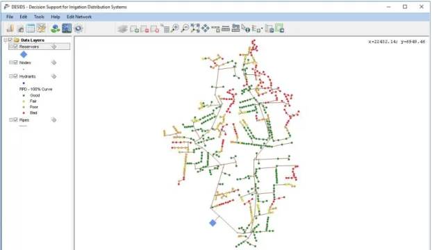
The developed DSS, called DESIDS (Decision Support for Irrigation Distribution Systems), is a stand-alone software, written in Microsoft® Visual Basic® programming language and
supported by a user-friendly graphical user interface (GUI) and built-in GIS capabilities (Fig. II-1). Prodigious care has been taken in creating a flexible, relatively easy to handle software, which could be used in different contexts of PIDS from planning to management and rehabilitation. DESIDS is set to address the different processes needed for managing collective irrigation systems (De Nys et al., 2008): operational (daily irrigation scheduling and distribution), tactical (changing systems’ operation without modifying the infrastructures) and strategic (changing structural capacities through new investments, e.g. structural rehabilitation). Therefore, it is set to help irrigation district managers address the different issues identified specifically in their districts.
14
DESIDS encompasses four separate, yet easily integrated elements or modules: i) an irrigation demand and scheduling module that calculates CWR, irrigation demand, irrigation scheduling for an entire irrigation district, and generates operating hydrants configurations; ii) a hydraulic analysis module that uses different PIs to evaluate the performance of a PIDS. The analysis is carried out by either randomly generating a large number of hydrant opening configurations or by using realistic configurations from the previous module; iii) an operation and management module that provide optimal operation strategies to achieve the best services (demand and pressure) to farmers; and iv) a rehabilitation module that implements multi-objective optimization for the rehabilitation of existing networks as well as the design of new ones. The outputs of each of the above modules are presented in tabular and graphical forms to facilitate the interpretation of the results. Some of the outputs are designed to be used as inputs for one of the available modules to enable the integration and the flow of information in the DSS as illustrated in Fig. II-2. Detailed descriptions of the four modules are presented in the following sections.
15
II.3 Irrigation demand and scheduling module
To evaluate the performance of PIDSs and to take the appropriate decisions concerning the operation and management of these systems, it is necessary to know the allocation of water at farm level. To this end, the irrigation demand and scheduling module is used to simulate CWR and irrigation scheduling for each field in an irrigation district. The incorporation of this module in DESIDS is imperative as it allows irrigation system managers to more efficiently match available discharges and pressures supplied by the system to on-farm water use. Thus, take the necessary decisions to provide adequate PIDSs performance to meet the crop water demand. Irrigation demand and irrigation scheduling are determined following the approach of CROPWAT using climatic, crop and soil parameters. The required data can be entered through the GUI and stored in a database to be retrieved when needed. All the input data and the results are displayed in tabular and graphical form to facilitate their interpretation (Fig. II-3). The estimation of irrigation requirements is one of the principal parameters for the planning, design, and operation of PIDSs. In this module, monthly available data are used to estimating the crop water and irrigation requirements, especially during the peak period, for a proposed cropping pattern for the planning and design of a PIDS. While the daily data if very important in formulating the policy for optimal allocation of water as well as in decision making in the day-to-day operation and management of the systems.
II.3.1 Irrigation Requirements
To estimate irrigation requirements, daily (or monthly) reference evapotranspiration (ET0) has
to be provided or calculated using either FAO-56 Penman–Monteith (Eq. II-1) or Hargreaves (Eq. II-2) methods, depending on the availability of data (Allen et al., 1998):
= 0.408 ∆ ( − ) +
900
+ 273 ( − )
∆ + (1 + 0.34 )
16
Fig. II-3. Irrigation demand and scheduling module
where Rn is the net radiation at the crop surface (MJ m-2 day-1), G is soil heat flux density (MJ
m-2 day-1), T is the mean daily air temperature at 2 m height (°C), u2 is the wind speed at 2 m
height (m s-1), es is the saturation vapour pressure (kPa), ea is the actual vapour pressure (kPa),
(es – ea) is the saturation vapour pressure deficit (kPa), Δ is the slope vapour pressure curve (kPa
°C-1), and γ is the psychrometric constant (kPa °C-1).
= 0.0023 ( + 17.8)( − ) . Eq. II-2
where Tmax and Tmin are, respectively, the maximum and minimum temperatures (°C), Ra is the
extraterrestrial radiation (mm day-1).
It is worth mentioning that, the values of crop evapotranspiration (ETc) and CWR are identical
herein, whereby ETc refers to the amount of water lost through evapotranspiration and CWR
refers to the amount of water that is needed to compensate for that loss. ETc is determined by
multiplying ET0 by the crop coefficient (Kc) provided for each growing stage. In this module,
17
The crop evapotranspiration under non-standard conditions, ETc,adj, is the evapotranspiration
from crops grown under management and environmental conditions that differ from the standard conditions. ETc,adj is calculated using a water stress coefficient (Ks).
The net irrigation requirement (NIR) is calculated as the difference between ETc,adj and the
effective rainfall. The latter can be estimated based on the provided rainfall data using four different options: i) fixed percentage of the actual rainfall; ii) FAO formula for dependable rainfall; iii) empirical formula; and iv) USDA Soil Conservation Service formula. It is also important to consider the losses of water, expressed in terms of efficiencies (Eirr), incurred
during irrigation application to the field. The gross irrigation requirement (GIR) is then calculated as:
= ⁄ Eq. II-3
II.3.2 Irrigation scheduling
Once the crops irrigation requirements have been calculated, the next step is the determination of irrigation scheduling. Concerning the latter, Pereira et al. (2003) recommended the use of soil water balance simulation when to be applied in the irrigation practice. For irrigation scheduling purposes, daily time steps are required because the irrigation managers are most often interested in estimating the irrigation depth and date(s) of application needed to maintain soil water content at a certain level. Three parameters have to be considered: the calculated daily CWR, the soil (particularly its total available moisture or water-holding capacity) and the effective root zone depth.
In this module, net irrigation depths are estimated using daily soil water balance expressed in terms of depletion at the end of the day (Allen et al., 1998):
= , − , − ( − ) − + + Eq. II-4
where Ii is the net irrigation depth on day i, Dr,iis the root zone depletion at the end of day i,
Dr,i-1 is water content in the root zone at the end of the previous day, i-1, Pi is the actual rainfall on day i, ROi is the runoff from the soil surface on day i, CRi is the capillary rise from the
18
groundwater table on day i, ETci is the crop evapotranspiration on day i, and DPi is the water
loss out of the root zone by deep percolation on day i, all expressed in mm. II.3.3 Generation of open hydrants configurations
To create a more realistic operation of hydrants in a PIDS, this module is set to generate hydrants’ configurations (hydrants operating simultaneously) for the entire irrigation season or a pre-defined period such as the peak period, using 15, 30 or 60 minutes time steps. After assigning each field in the irrigation district to a hydrant. The irrigation time can either be fixed by the user or generated randomly and the maximum irrigation time per day can also be limited if the PIDS is operated under rotation delivery schedule.
When it is time to irrigate, a hydrantj is opened and remains as such for the time of irrigation (tir,j), until the desired irrigation depth is delivered. On the other hand, when tir,j is greater than the operating time of the hydrant j, th,j (hours), irrigation scheduling for the entire season is adjusted to deliver the maximum possible irrigation depth, Imax,j (mm), and to fully satisfy
irrigation requirements:
, =
0.36 ,
Eq. II-5
where 0.36 is a units adaptation coefficient, qj is the nominal discharge of hydrant j (ls-1) and Ai is the area irrigated by hydrant j (ha)
All fields and the hydrants used to irrigate them are added to a table representing the irrigation scheme. In this module, the determination of the seasonal peak period is achieved by applying the moving average method to the daily volumes of irrigation water, for periods pre-defined by the user. The final step is the generation of hydrants’ opening configuration for the entire irrigation season or the period defined by the user. These configurations can be saved in a file to be used by the hydraulic analysis module.
19 II.4 Hydraulic analysis module
This module is the core of DESIDS, as it is the tool to evaluate the hydraulic performance of PIDSs and assess the impacts of their operations. This module combines the stochastic analysis capabilities for on-demand systems of COPAM (Lamaddalena and Sagardoy, 2000) and the analysis of complex systems using EPANET (Rossman, 2000) hydraulic solver to calculate unknown discharges and pressures for each operating hydrant in the considered PIDS.
There are two types of hydraulic analysis in WDSs: i) the demand-driven analysis (DDA), where the demands are assumed constant at hydrants regardless of the available pressure, thus it is not suitable for operating conditions with insufficient pressure (Tanyimboh and Templeman, 2010); and ii) the pressure-driven analysis (PDA), which considers the variation of demands depending on the pressure status. Several researchers have highlighted the use of PDA for its ability to deliver realistic results under different pressure conditions (D’Ercole et al., 2016; Giustolisi et al., 2009; Ozger and Mays, 2003).
II.4.1 Demand-Driven Analysis
The hydraulic analysis module assesses the performance of PIDSs using EPANET hydraulic solver, which is based on the conventional DDA. This solver is used by most of the developed models found in the literature to check the hydraulic feasibility of their generated solutions (De Corte and Sörensen, 2013). The solver provides the hydraulic analysis module with the ability to perform “extended period simulations”, which is used here for the simulation of hydrants operation for long periods of time (peak period or the entire irrigation season), by means of a succession of steady states.
Following the DDA formulation given in Todini and Pilati (1988), the Global Gradient Algorithm (GGA) is used to solve the mass and energy conservation laws. The general equation describing every element of a network is expressed as:
20
were
- Q = [Q1, Q2,…, Qnp]T = [np, 1] is a column vector of the computed pipe flows and np is
the number of pipes carrying unknown flows;
- H = [H1, H2,…, Hnn]T = [nn, 1] is a column vector of the computed nodal total heads
and nn is the number nodes with unknown pressure heads;
- H0 = [H01, H02, . . . ,H0n0]T = [n0, 1] is a column vector of the known nodal total heads
and n0 is the number of nodes with known pressure head (reservoirs);
- q =[q1, q2, . . . , qnn]T = [nn, 1] is a column vector of the nodal demands
In Eq. II-6, App represents a [np ,np] diagonal matrix whose elements are defined as=
( , ) = | | ∈ 1, Eq. II-7
while = and Ap0 are topological incidence submatrices, of size [np, nn] and [np, n0],
respectively, derived from the general topological matrix = | of size [np, nn + n0];
Rk is resistance factor for pipe k depending on whether the Darcy-Weisbach, Hazen-Williams
or Manning equation is used; and n is an exponent of the flow in the head loss equation (n = 2 for Darcy-Weisbach).
II.4.2 Pressure-Driven Analysis
In PIDSs, it is vital to deliver the minimum pressure at hydrants level required for the adequate functioning of on-farm irrigation systems and to supply the necessary water demand to meet irrigation requirements for the crops. In this context, the ability to perform PDA was added to the developed module to evaluate the actual discharges delivered by hydrants when the pressure at these hydrants is less than that needed to fully satisfy demand, hence, assess the effects of demand deficiencies at hydrant level on crops’ yield.
Several methodologies have been proposed for the application of PDA in WDSs:
1. Using the emitter element within EPANET for pressure driven modelling. However, the emitter has no upper limit for the discharge when the pressure is higher than the
21
minimum required pressure and it produces wrong results when the pressure is negative (negative discharges);
2. Embedding PDA in the governing network equations (Giustolisi et al., 2008; Muranho et al., 2014; Siew and Tanyimboh, 2012; Sivakumar and Prasad, 2014; Tanyimboh and Templeman, 2010);
3. Using DDA and iterating with successive adjustments made to specific parameters until a sufficient hydraulic consistency is obtained (Ozger and Mays, 2003); and
4. Using DDA with non-iterative methods by modifying the topological structure of the network, i.e., adding devices to the existing network such as valves, reservoirs, and emitters (Abdy Sayyed et al., 2015; Gorev and Kodzhespirova, 2013; Pacchin et al., 2016).
Nowadays, PDA is commonly employed in available WDSs models, which provide correct hydraulic analysis under both normal and pressure-deficient conditions. However, the majority of these models are fitted for drinking WDSs, e.g., for leakage modelling. The applications of this type of models in irrigation systems are seldom and only very few models are reported in the literature such as FLUC (Lamaddalena and Pereira, 2007) and GESTAR (Estrada et al., 2009).
For this study, the use of PDA in PIDSs is particularly important to assess the reliability of these systems when referring to their ability to provide the required discharges needed to meet on-farm water demands. To achieve this goal, the non-iterative method suggested by Abdy Sayyed et al. (2015) was applied in this module. This method was selected because it provides the possibility to perform PDA by directly using the EPANET toolkit with a single simulation. It was also compared to other similar method and applied on three real-life cases where it proved to provide accurate and reliable results, reproducing the functioning of a network in the pressure-driven mode (Pacchin et al., 2016)
The method consists of adding artificial string of check valve (CV), flow control valve (FCV), and emitter, in series, at each hydrant to model pressure deficient PIDS as illustrated in Fig. II-4.
22
Fig. II-4. Setting of the added devices for each open hydrant in the PDA
When the PDA option is selected for assessing the performance of a PIDS, the hydraulic analysis module automatically adds the abovementioned devices to all open hydrants following the procedure describe in Abdy Sayyed et al. (2015):
1. Add two nodes near to each open hydrant in the network. Add a CV pipe with negligible resistance between the hydrant and the first added node to restrict the negative flows, i.e., the length of pipe is given a very small value of 0.001. Add an FCV between first and second added nodes.
2. Make the base demand at all open hydrants as zero.
3. Set the elevation of both added nodes same as that of the corresponding hydrant. 4. Set the valve settings for each FCV to the demand at the corresponding hydrant. This
will restrict the hydrant discharge to the desired maximum.
5. The second added node is provided with emitter coefficient for the corresponding hydrant to simulate partial discharge condition. The module provides the option to set the emitter exponent to a single value for all hydrant or set different value for each hydrant.
6. The PDA is then performed where the hydrant is considered as a dead end. Consequently, for each hydrant, the resulting discharge is available at the emitter and the pressure at the hydrant.
II.4.3 Performance indicators
PIs are used to evaluate the hydraulic behaviour of a PIDS by quantifying its hydraulic reliability. In this module, four indicators are used in order to efficiently analyse the performance of the analysed PIDS:
Relative Pressure Deficit, RPD (Lamaddalena and Sagardoy, 2000): the actual pressure head for hydrant j (Hj) is compared with the minimum pressure (Hmin,j), required at the same hydrant for an appropriate on-farm irrigation. Thus, the hydraulic performance for each
23
hydrant j is obtained through the computation of the relative pressure deficit defined hereafter.
= − ,
,
Eq. II-8
with the RPD, the range of variation of the pressure head at each hydrant is determined and consequently, the critical zones of the system are identified.
Reliability, Re (Lamaddalena and Sagardoy, 2000): it indicates the ability of a PIDS to provide an adequate level of service, referring to the pressure, to farmers under several operating conditions and within a pre-defined operation time. Hence, this indicator is calculated as the probability that the pressure at any hydrant in the network is at or above the minimum required pressure. Therefore, Rejis calculated as the probability that the hydrant j is in a satisfactory state (Hj ≥ Hmin,j):
= , ,
Eq. II-9
where Ns,j is the number of times the pressure at hydrant j is satisfied and No,j is the total number of times where hydrant j is open.
During a DDA simulation of PIDSs, it is not possible to use PIs based on water demands delivered to farmers because the demands remain fixed, i.e., not dependent of pressure (Laucelli et al., 2012). Using PDA, two additional PIs were added to quantify demands deficit at hydrant and network levels. These were added to the module because they have a physical interpretation unlike the reliability based on pressure deficiencies.
Available Discharge Fraction ADF (Ozger and Mays, 2003): the available discharge at hydrant j (qj,avl) is compared with the required discharge (qj,req), at the same hydrant, set to meet
the irrigation requirements at farm level. Hence, this indicator is used to estimate the fraction of the discharge that is actually delivered by hydrant j.
24
= ,
,
Eq. II-10
Available Volume Fraction AVFnet: this indicator is used to assess the reliability of the entire
irrigation network and is calculated as:
= Eq. II-11
were Vact and Vreq are the total volume of water actually supplied by the network and the
total volume required to be supplied (m3), respectively.
II.4.4 Assessment of the hydraulic performance
The assessment of the hydraulic behaviour of a PIDS can be accomplished using the hydraulic analysis module given the topology of the network, the geometry of the pipes, the discharges delivered by the hydrants and the required minimum pressure at these hydrants. When importing this information, from MS-Access® database, DESIDS uses the coordinates of each node to
create shapefiles for all elements of the network and displays them in the integrated GIS environment (Fig. II-1).
The module analyses PIDSs under several operation scenarios. This is attained by either deterministic or random configurations of hydrants operating (open) simultaneously. The former is generated using the irrigation demand and scheduling module described above, while the latter is generated randomly by the hydraulic analysis module considering predefined upstream discharges (Fig. II-5). Thus, the total number of open hydrants in each configuration has to respect the following constraint:
25
where Nhyd is the total number of open hydrants, qj is the nominal discharge of the hydrant j
selected randomly, and Qup is the upstream discharge at the head of the network.
Fig. II-5. Hydraulic analysis module
When the operating hydrants scenarios are available (defined by a certain number of configurations Nconf), the user of DESIDS can run either a DDA or PDA according to the
intended outcomes. That is if pressures at some hydrant fall below a minimum required level, the flow will be significantly reduced. In this case, PDA can be used to account for both pressure and demand deficiencies in the PIDS.
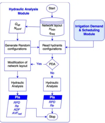
As abovementioned, the module uses EPANET toolkit for the analysis process. Therefore, to avoid calling the toolkit in each analysed configuration, the module automatically generates the input file for EPANET considering each configuration as a time step in an extended period simulation. The results of the analysis are then sorted and the generated PIs are presented in graphical and tabular forms to facilitate their interpretations. The process of the hydraulic analysis used in the module is presented in Fig. II-6.
26
Fig. II-6. Flowchart of the hydraulic analysis module
II.5 Operation and management module
PIDSs are facing mounting burden to provide solutions to the increasing water demand at farm level. Therefore, the operation and management of these systems are crucial factors to achieve an efficient use of both, the available water and the capacity of the systems to deliver the necessary pressures and demands to meet the requirements of on-farm systems and crops. When designing PIDSs operating on-demand, it is a common practice to calculate the probability of hydrants operation patterns using methods such that proposed by Clément (1966). However, the foremost challenge in managing these systems in actual situations is to identify ahead of time the flows into the networks’ pipes, which are random and depend on the behaviour of farmers. In fact, even when the design flows are not exceeded, very low hydraulic performance can occur in these systems during their operation (Lamaddalena and Pereira, 2007).
To this end, the aim from developing the operation and management module is to provide irrigation district managers with a useful tool, which can be effectively used in finding solutions
27
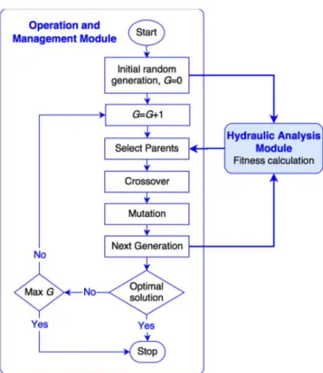
to PIDSs management under a wide range of scenarios. These solutions allow the improvement of the actual operation as well as the sustainability of these systems. Accordingly, this module offers optimal management strategies for PIDSs through the smooth transition to rotation delivery schedule for systems designed for on-demand when they are facing performance problems, especially during the peak irrigation demand periods. The module uses Genetic Algorithm (GA) for the optimization of irrigation periods taking into account, the minimization the pressure deficit at the most unfavourable hydrant as objective function (Fig. II-7).
Fig. II-7. Optimization of irrigation periods II.5.1 Genetic Algorithms
GAs (Goldberg, 1989) are powerful metaheuristic search methods used for solving both constrained and unconstrained optimization problems, based on a natural selection process that mimics natural evolution. They use the same combination of selection, recombination and mutation to evolve a solution to a problem. These methods have been applied to the solution of many optimization problems in WDSs (Farmani et al., 2007; Reca and Martínez, 2006; Savic and Walters, 1997), because of the easy use of their properties and their robustness in finding good solutions to difficult problems.
28
GAs start with a randomly generated initial population, i.e., a set of solutions represented by chromosomes, which evolves through three main operators: i) the selection, where chromosomes are selected from the population according to their fitness values to be parents; ii) crossover, where some genes from parent chromosomes are selected to create new offspring. This is done by randomly choosing one or more crossover point(s) where a pair of parent chromosomes exchange information; and iii) mutation, which changes randomly the new offspring to retain the diversity of the solution in a population and expand the search in the solution space.
II.5.2 Optimization of irrigation periods
The main objective from this module is to offer irrigation district managers a tool to obtain the optimal operation of PIDSs when the latter are facing performance problems. The optimization process is carried out using GA. The module starts with a population of randomly generated individuals (chromosomes), each representing a possible solution that has to be evaluated by means of the considered objective function, which is the minimization of the pressure deficit at the most unfavourable hydrant in the network. The number of variables (genes) within the individuals is determined by the number of open hydrants randomly generated while the values of these variables depend on the number of irrigation periods. In another word, each open hydrant is randomly assigned to an irrigation period. Therefore, the value of each variable ranges between 1 and the number of open hydrants.
The initial population is then evaluated by performing a hydraulic simulation, using the hydraulic analysis module, for each individual to obtain the pressure head of the open hydrants. The pressure deficit at the most unfavourable hydrant is then assigned to each individual and used as its fitness value. Based on their fitness, individuals with the lowest pressure head deficit (fitter solutions) are selected as parents and used to create new individuals (offspring) for the next generation. This is achieved through the processes of crossover and mutation. The crossover process implies that a pair of parent individuals exchange information in order to produce a pair of offspring individuals that inherit their characteristics. Herein, this process is done using a one-point crossover procedure, which entails that randomly selected pairs of parent individuals exchange information to produce offspring. The crossing point, that cuts both parent