Dottorato di Ricerca in Bioingegneria
XX CICLO
Settore Scientifico Disciplinare: ING-IND/34
BIOMECHANICAL MODELLING OF HUMAN KNEE
DURING LIVING ACTIVITIES
(MODELLAZIONE BIOMECCANICA DEL GINOCCHIO DURANTE ATTIVITA’ MOTORIE QUOTIDIANE)
Autore
Ing. Luigi Bertozzi
Coordinatore
Prof. Angelo Cappello
Supervisore
Prof. Angelo Cappello
Correlatore
Prof. Rita Stagni
Controrelatore
Prof. Luca Cristofolini
Esame finale anno 2008
L’articolazione di ginocchio è una struttura chiave del sistema locomotore umano. Conoscere come ogni singola struttura anatomica contribuisce a determinare la complessa funzione biomeccanica del ginocchio è di fondamentale importanza per lo sviluppo di nuove protesi e di innovative procedure cliniche, chirurgiche e riabilitative. In questo contesto, l’utilizzo di un approccio modellistico è l’unico modo possibile per quantificare la funzione biomeccanica di ogni singola struttura anatomica in condizioni fisiologiche, come ad esempio stimare la forza prodotta dai legamenti crociati durante l’esecuzione di compiti motori quotidiani.
Lo scopo principale di questo studio è stato ottenere un modello di ginocchio altamente specifico di un soggetto selezionato utilizzando tecniche diagnostiche per immagini, come risonanza magnetica e video-fluoroscopia. Utilizzando accurate geometrie ossee e cinematiche articolari acquisite sperimentalmente dal soggetto considerato, sono stati sviluppati modelli 3D dei legamenti crociati e del contatto articolare tra tibia e femore.
Nel modello dei legamenti crociati, ognuno dei due legamenti è stato modellato tramite l’utilizzo di 25 elementi elastici-lineari disposti considerando la naturale torsione anatomica delle fibre. Nel modello sviluppato si è cercato di raggiungere il più alto livello di specificità al soggetto possibile. Infatti, ogni singola molla è stata geometricamente caratterizzata utilizzando dati sperimentali provenienti dal soggetto selezionato, mentre l’unico parametro meccanico del modello, il modulo elastico, è stato considerato da dati sperimentali riportati in letteratura a causa delle misure invasive necessarie per quantificarlo nel soggetto selezionato. Una volta implementato, il modello è stato utilizzato simulando test di stabilità e imponendo i compiti motori eseguiti dal soggetto. I risultati ottenuti sono sempre stati fisiologicamente significativi. Tuttavia, la mancanza di un valore del modulo elastico proveniente dal soggetto selezionato ha generato la necessità di sviluppare una metodologia sperimentale per caratterizzare la meccanica dei legamenti crociati in soggetti viventi e senza misure dirette ed invasive.
Utilizzando i medesimi dati geometrici e cinematici, sono stati anche implementati due modelli per la valutazione del contatto tibio-femorale, uno finalizzato alla stima dell’area di contatto in posizioni statiche (massima estensione con e senza peso corporeo), ed uno finalizzato alla valutazione della posizione del punto di contatto durante i compiti motori eseguiti dal paziente. Questi due diversi approcci sono stati implementati e testati valutando i pro e i contro di ognuno in modo da suggerirne il corretto ambito di utilizzo e possibili miglioramenti futuri.
Il risultato finale di questo studio contribuirà allo sviluppo di avanzate metodologie per la valutazione in-vivo della funzione/patologia dell’articolazione di ginocchio, anche durante compiti motori della vita quotidiana. Le metodologie sviluppate saranno così di notevole utilità per lo sviluppo di nuove protesi, strumenti e procedure sia nel campo della ricerca che in campo clinico, chirurgico e riabilitativo.
The knee joint is a key structure of the human locomotor system. The knowledge of how each single anatomical structure of the knee contributes to determine the physiological function of the knee, is of fundamental importance for the development of new prostheses and novel clinical, surgical, and rehabilitative procedures. In this context, a modelling approach is necessary to estimate the biomechanic function of each anatomical structure during daily living activities.
The main aim of this study was to obtain a subject-specific model of the knee joint of a selected healthy subject. In particular, 3D models of the cruciate ligaments and of the tibio-femoral articular contact were proposed and developed using accurate bony geometries and kinematics reliably recorded by means of nuclear magnetic resonance and 3D video-fluoroscopy from the selected subject.
Regarding the model of the cruciate ligaments, each ligament was modelled with 25 linear-elastic elements paying particular attention to the anatomical twisting of the fibres. The devised model was as subject-specific as possible. The geometrical parameters were directly estimated from the experimental measurements, whereas the only mechanical parameter of the model, the elastic modulus, had to be considered from the literature because of the invasiveness of the needed measurements. Thus, the developed model was employed for simulations of stability tests and during living activities. Physiologically meaningful results were always obtained. Nevertheless, the lack of subject-specific mechanical characterization induced to design and partially develop a novel experimental method to characterize the mechanics of the human cruciate ligaments in living healthy subjects.
Moreover, using the same subject-specific data, the tibio-femoral articular interaction was modelled investigating the location of the contact point during the execution of daily motor tasks and the contact area at the full extension with and without the whole body weight of the subject. Two different approaches were implemented and their efficiency was evaluated. Thus, pros and cons of each approach were discussed in order to suggest future improvements of this methodologies.
The final results of this study will contribute to produce useful methodologies for the investigation of the in-vivo function and pathology of the knee joint during the execution of daily living activities. Thus, the developed methodologies will be useful tools for the development of new prostheses, tools and procedures both in research field and in diagnostic, surgical and rehabilitative fields.
The successful completion of this work is the result of the help, cooperation, faith and support of many people.
First of all, I need to thank my supervisor Prof. Angelo Cappello, since without him, none of this work would have been possible. He provided me with the opportunity to make this research happen.
A special thanks to my co-supervisor, Prof. Rita Stagni, for her great patience, constant encouragement, and endless support throughout my doctoral studies. Her patient guidance not only helped me to improve my research skills, but also to become a better person.
For their reviews and comments regarding the manuscript you are holding, I would like to thank Prof. Silvia Fantozzi and Prof. Luca Cristofolini. The suggestions they provided helped me to greatly improve the quality of this document.
I would also extend my sincere appreciations to all my friends who stayed close to me in these years. In particular, I would to thank Luca for the pleasant conversations, the restoring walks and swims, and the hard fought games of chess.
My parents receive my deepest gratitude and love for their many years of support and encouragement.
Last but not the least, I would like to thank my wife for her understanding and love during the past few years, and specially for giving me a beautiful daughter, Rita.
Abstract – Italian Version i Abstract iii Acknowledgements v Table of Contents vi List of Tables ix List of Figures x
List of Abbreviations xiv
Introduction 1
References 4
Chapter 1: Description of Knee Joint 5 1.1 General Anatomical References 5 1.2 Anatomy, Morphology, and Mechanics 8 i Bones 8
ii Joints, Ligaments and Menisci 10 iii Structure and Mechanics of Knee Ligaments 15 iv Muscles 20 1.3 Biomechanics: functional anatomy 25 i Mobility 25
ii Stability 30
1.4 References 32
Chapter 2: Review of Knee Models 37
2.1 Kinematical Models 38
2.2 Static and Quasi-Static Models 40 2.3 Dynamic Models 47
2.4 Proposal for Innovative Approaches 51
i Model of Cruciate Ligaments 52
i Selected Subject and Experimental Acquisitions 62 ii Reconstruction of Subject-Specific Data 63 iii Geometrical Aspects of the Model 64 iv Mechanics of Ligaments and Definition of Parameters 67
v Simulations 69
3.2 Results 71
i Drawer Test 71
ii Axial Test 76
iii Daily Living Activities 78
3.3 Discussion 79
3.4 Conclusions 82
3.5 References 85
Chapter 4: Model of Tibio-Femoral Contact 91
4.1 Materials and Methods 92
i Subject, Experimental Acquisitions, Data Reconstruction 92 4.2 Thin Plate Splines for Static Evaluations of Proximity 92 i Preliminary Elaborations of the Experimental Data 92 ii Using TPS to Describe Bony Surfaces 93 iii Distance between Surfaces and Contact Area Estimations 97 iv Results for Static Positions With and Without Body Weight 100
v Discussion 104
4.3 3D Distance Maps for Quasi-Static Evaluations of Proximity 107 i 3D Distance Map: Construction and How It Works 108 ii Proximity Between Femur and Tibia During Living Tasks 111
iii Results 113
iv Discussion 115
4.4 Conclusions 119
Ligaments 125
5.1 Knee Laxity Measuring Device 125
5.2 Preliminary Developments 127
i Results 129
ii Discussion 131
5.3 Conclusions and Future Works 132
5.4 References 134
Conclusions 135
List of Publications 143
Table 3.1: Parameters of the NMR scanning-procedure. 63
Table 4.1: Contact areas estimations, with mean values and standard deviations, obtained for the three positions of the knee loaded at the full
Figure 1.1: Anatomical planes and axis. 6 Figure 1.2: Joint angles are defined by rotations occurring about the three joint coordinate axes. Flexion/extension is about the femoral body fixed axes. External/internal tibial rotation is about the tibial fixed axis and ab/adduction is
about the floating axis (F). 6
Figure 1.3: Human knee joint. 7 Figure 1.4: Lower extremity of right femur viewed from below (Gray, 1918). 9 Figure 1.5: Upper surface of right tibia viewed from above (Gray, 1918). 9 Figure 1.6: Right knee-joint. Anterior view (Gray, 1918). 11 Figure 1.7: Right knee-joint, from the front, showing interior ligaments (Gray,
1918). 12
Figure 1.8: Left knee-joint from behind, showing interior ligaments (Gray,
1918). 13
Figure 1.9: Head of right tibia seen from above, showing menisci and
attachments of ligaments (Gray, 1918). 15 Figure 1.10: Schematic diagram of the hierarchic structure of ligament. The
whole ligament is composed of fibre bundles even more small up to reach the
basic structural element, which is the tropocollagen molecule. 16 Figure 1.11: Example of a force-elongation curve obtained from a
bone-ligament-bone specimen. Four regions are commonly used to describe a force-elongation or stress-strain curve. Region 1 is termed the "toe region" and elicits a non-linear increase in load as the tissue elongates. Region 2 represents the linear region of the curve. In Region 3, isolated collagen fibres are disrupted
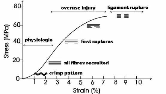
and begin to fail. In Region 4, the ligament completely ruptures. 17 Figure 1.12: Example of stress-strain curve to describe the relationship
between changes in the collagen "crimp" pattern, or stretch, and ligament mechanical properties. An increasing of the strain in the ligament at the "toe region" of the curve produces a straightening of the "crimp" pattern. During the linear portion of the curve, the collagen fibres are stretched more and more with the increasing of the strain. As the ligament is further strained isolated ligament fibres begin to rupture and if deformation continues, then complete
ligament fail occurs. Modified from (Butler et al., 1978). 18 Figure 1.13: A hypothetical force-elongation curve for a human ACL-bone
complex is illustrated along with daily activities that correspond to specific loading levels. During routine daily activities such as walking and standing, ligaments are loaded to less than one fourth their ultimate tensile load. During strenuous activities such as fast cutting during intense running, loading levels may enter into region 3 where isolated fibre damage takes place. Modified
from (Noyes et al., 1984). 19
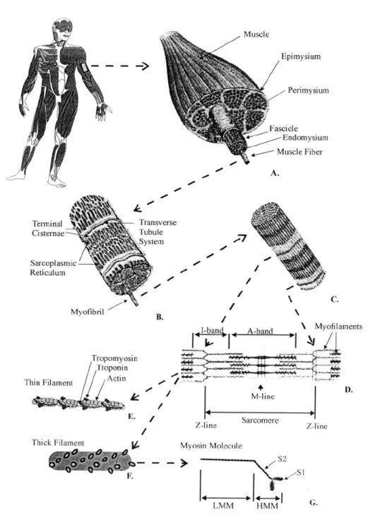
Figure 1.14: Schematic representation of the organizational structure of muscle. The gross muscle is composed of bundles of fascicles that consist of groups of fibres. Fibres can be further divided into myofibrils that contain the
myofilaments making up the sarcomeres. 21 Figure 1.15: Anterior (a, c ) and posterior (b, d) views of muscles of a right
tibial attachment sites, and CA designates the femoral insertion points. The flexion axis is the point of intersection at each instant between the links AB
and CD (Kapandji, 1970). 26
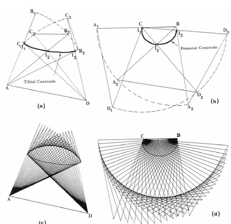
Figure 1.17: The cruciate linkage drawn by the computer with the tibial link fixed, (a) and (c), and with the femoral link fixed, (b) and (d). the relative positions of the links are the same in the pair of diagrams (a) and (b) for each of the corresponding three configurations and in (c) and (d) for each of the corresponding 30 configurations. In (a) and (c), the femoral attachments of the ligaments move on circular arcs about their tibial attachments, and in (b) and (d) the tibial attachments move on circular arcs about the femoral attachments. The curve marked “Tibial centroide” and “Femoral centroide” are the tracks of the flexion axis of the joint on the tibia and femur, respectively, and are drawn
through the successive intersections of the cruciates (O'Connor et al., 1990). 27 Figure 1.18: From 0 to 10-15°, the motion is predominantly rolling (A), from
10-15° to 140-160° sliding (B) (Kapandji, 1970). 28 Figure 1.19: The diagram shows the cruciate linkage in two neighboring
positions with the corresponding femoral surface touching a flat tibial plateau at F and F’. F’’ is the point on the femoral surface which makes contact with F. The slip ration is the distance F’F’’ measured along the femur, divided by the distance FF’ measured along the tibia. The graphs show the variation with flexion angle for convex, flat and concave tibial plateaus (O'Connor et al.,
1990). 28
Figure 1.20: The screw-home mechanism: coupled internal rotation of 20° of
the tibia on the femur during knee flexion (Kapandji, 1970). 29 Figure 1.21: Functioning of the menisci: Sliding movements between the
femur and the concave upper surface of the menisci allow flexion and extension, sliding movements between the flattened undersurface of the meniscus and the tibial plateau allow rotation and anteroposterior translation of
the tibia (Kapandji, 1970). 29
Figure 3.1: Anterior (a) and posterior view (b) of the bony segments
reconstructed by NMR. Ligament insertion areas (dotted regions) on the femur and the tibia (c) from an anterior viewpoint. From Bertozzi et. al (Bertozzi et
al., 2006c). 64
Figure 3.2: Example of an anatomical insertion area with the 25, insertion points, fitted in 3D by TPS method, and the two elliptical contours. From
(Bertozzi et al., 2006c). 66
Figure 3.3: Ordering pattern relative to the Anterior Cruciate Ligament (a)
and the Posterior Cruciate Ligament (b). 67 Figure 3.4: Laxity calculated at ±200N at different flexion angle and
superimposed with the experimental data reported by Markolf et al. in 1978 and 1981. Mean values (full dots) plus and minus two standard deviations
(vertical bars) were shown for experimental results. 72 Figure 3.5: Anterior Stiffness calculated at different flexion angle and
superimposed with the experimental data reported by Markolf et al. in 1978 and 1984. Mean values (dots) plus and minus two standard deviations (vertical
and 1984. Mean values (dots) plus and minus two standard deviations (vertical
bars) were shown in figure. 74
Figure 3.7: Laxity calculated at ±100N (a), Neutral Stiffness (b), Anterior Stiffness (c) and Posterior Stiffness (d) calculated considering 30% (o), 60% (*) and 100% (+) of the in-vivo estimated cross-sectional area value versus flexion angle. Predictions compared with the experimental measurements reported by Markolf et. al (Markolf et al., 1976; Markolf et al., 1978; Markolf
et al., 1981; Markolf et al., 1984; Shoemaker and Markolf, 1985). 75 Figure 3.8: Internal/external tibial torque versus internal/external axial rotation drawn at 0° (a), 10° (b), 25° (c) and 45° (d) of flexion. Three curves were plotted considering different elastic modulus values: mean value (+), mean value minus one standard deviation (*) and mean value plus one standard
deviation (x) (Butler et al., 1992; Race and Amis, 1994). 76 Figure 3.9: Anterior/posterior component forces provided by PCL versus the
knee flexion angle: two repetitions of extension (A) and flexion (C) motions during step up/down motor task, nine repetitions of extension (B) and flexion
(D) motions during chair rising/sitting motor task. 77 Figure 3.10: Medial/lateral component forces provided by the posterior
cruciate ligament versus the knee flexion angle: two repetitions of extension (left) and flexion (right) motions during step up/down motor task evaluated
using the two definitions of the Elastic Modulus parameter. 79
Figure 4.1: Experimental points of the lateral condyle projected on the xy plane (blu asterisks). The region R (green rectangle), region D (red dashed line), grid nodes inside and outside the region D (azure circles and little black
dots, respectively) are depicted. 94
Figure 4.2: Final form of the TSP of the lateral condyle (colored mesh) with
outgoing normals calculated at grid nodes (blue arrows). 95 Figure 4.3: Femoral and tibial original geometries (little green and yellow
dots, respectively). The selected femoral points and the relative femoral TPS (blue points and meshes) for the lateral and the medial side (left and right). The selected tibial points and the relative tibial planes (red points and planar grids). 99 Figure 4.4: Bottom-rear sight of the lateral TPS (colored mesh) and estimated
contact area (blue region) obtained without body weight with Dth= 3 mm and
M = 40. 99
Figure 4.5: Estimations of the femoral (a) and the tibial (b) contact areas on the lateral side in function of the Dth parameter. Percentage, on the total
number, of the normals outgoing from the femoral TPS which take part of the contact zone (c). Curves obtained with different values of the M parameter are
shown. 101
Figure 4.6: Estimations of the femoral (a) and the tibial (b) contact areas on the medial side in function of the Dth parameter. Percentage, on the total number, of the normals outgoing from the femoral TPS which take part of the contact zone (c). Curves obtained with different values of the M parameter are
(a) and the medial (b) side. Curves obtained with different values of the Dth
parameter are shown. 103
Figure 4.8: Scheme of the lateral distance map. Lateral tibial plateau (gray) is bounded by the Domain of the distance map (yellow rectangle). A node of the map (red), some tibial points (violet) and the tibial point closest to the
considered node (azure) are shown. 109 Figure 4.9: Scheme of the estimation of the distance (blue) of a femoral point
(black) from the tibial plateau (azure) by means of the use of the distance map (red). From the spatial coordinates of the femoral point, the eight map nodes closest to the point (red) is identified. The estimation of the distance is performed with a tri-linear interpolation of the distances stored at the eight nodes. Here, all eight nodes point at the same tibial point (azure) but, generally, each node can point at a different tibial point. At the end, the final tibial point (azure), which is closest to the considered femoral point, is estimated as the
barycentre of all tibial points obtained. 110 Figure 4.10: Colored proximity map between the femur and the tibia at the full
extension position [mm]. 112
Figure 4.11: Anterior-posterior translation of the lateral (left) and the medial (right) contact points during the execution of the step up/down motor task with
the extension (top) and the flexion (bottom) movements detached. 114 Figure 4.12: Anterior-posterior translation of the lateral (left) and the medial
(right) contact points during the execution of the chair rising/sitting motor task
with the extension (top) and the flexion (bottom) movements detached. 114
Figure 5.1: Whole scheme of the devised methodology to implement the
subject-specific model of the cruciate ligaments of a living healthy subject. 126 Figure 5.2: Mechanical device for the quantization of the drawer test: handle
for the manual application of forces and torques (a), Bertec six-component load transducer (b), commercial rigid tibial brace (c), temporary coupling system (d). The test of the temporary coupling system was performed with
stereo-photogrammetric acquisitions performed in a gait analysis laboratory. 128 Figure 5.3: Distal(-)/Proximal(+) (X), Lateral/Medial (Y) and
Posterior/Anterior (Z) tibial components of the forces acquired in the reference
system of the load cell. 130
Figure 5.4: Flexion(-)/Extension(+) (X), External/Internal (Y) and
Abduction/Adduction (Z) tibial torques acquired in the reference system of the
load cell. 130
Figure 5.5: Anterior stiffness obtained during the third test and calculated from
2D: Two-dimensional 3D: Three-dimensional A/P: Anterior-Posterior direction/axis M/L: Medial-Lateral direction/axis P/D: Proximal-Distal direction/axis Lg: Longitudinal direction/axis Fl/Ex: Flexion-Extension angle/rotation In/Ex: Intra-Extra angle/rotation (I/E) Ab/Ad: Abduction-Adduction angle/rotation
NMR: Nuclear Magnetic Resonance MRI: Magnetic Resonance Imaging CT: Computed Tomography EMG: Electromyography EEG: Electroencephalography GFR: Ground Force Reaction
ACL: Anterior Cruciate Ligament PCL: Posterior Cruciate Ligament MCL: Medial Collateral Ligament LCL: Lateral Collateral Ligament
DAEs: Differential Algebraic Equations RBSM: Rigid Body Spring Model FEM: Finite Element Method MH: Modified Hertzian theory SES: Simplified Elastic Solution TPS: Thin Plate Splines
NURBS: Non-uniform rational B-splines RMSE: Root Mean Square Error
Introduction
The human knee joint is an attracting complex of anatomical structures which fascinates anatomists, clinicians and bioengineers. This joint has two apparently contrasting requirements: it must be mobile in order to achieve a large and smooth range of motion, and it must be stable in order to guarantee strong support to loading conditions of the daily living activities. The knee accomplishes these two fundamental requirements by the concurrent actions of different active (i.e. muscles), and passive anatomical structures, such as the cruciate ligaments, and by the conformity of the articular surfaces. Any injury to any of these anatomical structures alters the function of the whole joint. Thus, a good knowledge of the in-vivo biomechanical function of each anatomical sub-unit is of fundamental importance and of great clinical interest for the development of new effective rehabilitative and surgical procedures.
In order to reach this aim, it is possible to use different approaches. Although experimental methods produce direct and reliable measurements of the variables of interest, they are usually quite invasive and can alter physiological conditions and limit generalization. Thus, when the goal is the evaluation of the normal function of the considered organ, invasive measurements should be avoided and a modelling approach might be preferred. Moreover, with the evolution of the medical and the diagnostic technologies, such as MRIs, CTs, EMGs and EEGs, nowadays it is possible to investigate the anatomy and the function of organs and tissues of a living healthy subject with a limited invasiveness.
The aim of this work was to provide novel experimental methodologies for the investigation of the knee joint in living subjects, with particular attention to the subject-specific modelling of the cruciate ligaments and of the tibio-femoral contact. Thus, the objective of this study was to obtain subject-specific models of the cruciate ligaments and of the tibio-femoral articular interaction, which were exploitable during the execution of daily living activities. Each one of these models was designed and developed as a computational tool aimed to investigate the specific functionality/pathology
of the considered anatomical structure of the selected subject. This means that, for example, the model of the cruciate ligament neglected the possibility to evaluate the functionality of other anatomical structures of the knee, such as collaterals, capsule, muscles and bony and cartilaginous interactions. Moreover, each developed model neglected the possibility: i) to export the developed methodology for other similar anatomical structures, because of the specificity of the hypotheses made with respect to the considered anatomical structure, and ii) to generalize the model designed for a specific subject and apply it for other subjects, because of the intrinsic differences in morphological and kinematical data. Finally, since the developed models were aimed to be used in physiological conditions, such as the execution of daily living activities, these models had to be simple and computationally light in order to be executed several times, once for each acquired frame. In this study, the considered kinematics were only the chair rising/sitting and the step up/down motor tasks, but using the developed methodologies and models can be evaluated all those motor tasks in which the knee under analysis can be recorded by means of a video-fluoroscopy.
The terminology used in the present thesis with respect to the biomechanics of knee joint is provided in Chapter 1. In particular, an anatomical description of the main passive and active structures is provided paying a particular attention on the mechanical behaviour of the modelled anatomical structures. Finally, a brief biomechanical description of the two apparently conflicting functions of the physiological knee joint (i.e. stability and mobility) is also proposed.
Through the last two centuries, the problem of the knee modelling has been tackled from different points of view and at different levels of complexity. A thorough state-of-the-art review about knee biomechanics is reported in Chapter 2. A particular attention is focused on methods and tools that can be used in modelling of knee joint and on problems that could arise in this context.
The cruciate ligaments are one of the most attractive anatomical structures of the knee joint because of their mechanical behaviour, which is simple but very effective and hard to reproduce by means of the surgical approach. The interest on these anatomical structures is also demonstrated by
9000 other repair of cruciate ligaments performed in the USA in 2004 as reported by the American Association of Orthopaedic Surgeons (AAOS). Given the importance of these key structures, a 3D quasi-static model of the human cruciate ligaments is implemented and described in Chapter 3. The devised model is as subject-specific as possible, because it is extensively based on the use of geometrical and kinematical data acquired and computationally reconstructed from a living and healthy selected subject. This model is also used to evaluate the functionality of the cruciate ligaments both during simulated stability tests, and during the execution of daily living activities.
Another important mechanism of the knee joint is the interaction between the tibial and the femoral bones, the tibio-femoral joint. This mechanism, along with the cruciate ligaments, is one of the most important to provide knee joint with its two main functions: stability and mobility. Thus, using the same geometries and same the kinematics acquired and reconstructed for the cruciate ligament model, two different approaches to evaluate the 3D tibio-femoral interaction in living subjects are provided in Chapter 4.
Considering again the cruciate ligaments model described in Chapter 3, the only two aspects, that prevented to obtain a validated subject-specific model, are the lack of the subject-specific elastic modulus and the knowledge of the forces produced from the cruciate ligaments of the selected subject during the kinematical acquisition. In order to overcome these two problems, in Chapter 5, a novel experimental arthrometer, a device with the capability to synchronously measure the forces applied to the knee and the joint kinematics, is proposed and developed at a prototype stage.
When all devised methodologies will be improved and integrated, this study will provide the biomechanical and the clinical communities with useful methodologies for the evaluation of the in-vivo function and pathology of the knee joint in living subjects, with the capability to perform estimations during the execution of daily living activities. Moreover, the developed methodologies will be useful tools for the development of new prostheses, tools and procedures both in research field and in diagnostic, surgical and rehabilitative fields.
References
AAOS, American Association of Orthopaedic Surgeons, 2004 Available on-line at http://www.aaos.org/Research/stats/patientstats.asp
Chapter 1:
Description of Knee Joint
In this chapter, a comprehensive description of the human knee joint is provided in order to better understand the terminology used in next and more specific chapters. First of all, anatomical and articular references are defined with respect to specific clinical and anatomical studies (Gray, 1918; Gray, 1977; Grood and Suntay, 1983). Then, the main structures of the knee joint, such as bones, ligaments and muscles, are deeply described from an anatomical and morphological point of view. A description of the mechanical behaviour is also provided for those anatomical structures considered of major interest in this study. Finally, in order to help the reader, a short survey about the biomechanics of the knee joint is provided paying particular attention to its main functions, the stability and the mobility.
1.1 General Anatomical References
Before specifying the anatomy of the knee joint in detail, in this section the terminology used in the present thesis to define kinematics terms is reported. For descriptive purposes, the body is usually supposed to be in the erect posture, with the arms hanging by the sides and the palms of the hands directed forward (Figure 1.1). The median plane is a vertical anterior-posterior (AP) plane, passing through the centre of the trunk, approximately through the sagittal suture of the skull, and hence any plane parallel to it is termed a sagittal plane. A vertical plane at orthogonal to the median plane passing through the central part of the coronal suture or through a line parallel to it is known as a coronal plane. A plane at right angles to both the median and frontal planes is termed a transverse plane. The terms anterior, and posterior, are used to indicate the relation of parts to the front or back of the body or limbs (anterior-posterior axis, AP axis), and the terms superior, and inferior, to indicate the relative levels of different structures (along the longitudinal axis, Lg axis). Structures nearer to or farther from the median plane are referred to as medial or lateral respectively (along the medio-lateral axis, ML axis). In the case of the limbs the words proximal and
distal refer to the relative distance from the attached end of the limb (along
mCORONAL PLANE mLONGITUDINAL AXIS mMEDIO-LATERAL AXIS MEDIAN PLANE o ANTEROPOSTERIOR o AXIS TRANSVERSE o PLANE
Figure 1.1: Anatomical planes and axis
INTERNAL (+) EXTERNAL (-) ABDUCTION (+) ADDUCTION (-) EXTENSION (-) FLEXION (+) F
Figure 1.2: Joint angles are defined by rotations occurring about the three joint coordinate axes. Flexion/extension is about the femoral body fixed axes. External/internal tibial rotation is about the tibial fixed axis and
According to the ISB recommendations (Wu and Cavanagh, 1995), the knee joint coordinate system used in the present thesis allows rotations about axes which can be anatomically meaningful, allowing the preservation of an important linkage with medical terminology. The system used was the one proposed by Grood and Suntay (Grood and Suntay, 1983) (Figure 1.2). Two body fixed axes are established relative to anatomical landmarks, one in each body on opposing sides of the joint: one is the medio/lateral axis of the femur the other is the longitudinal axis of the tibia (Figure 1.2). The third axis, called the floating axis (Figure 1.2, F), is defined as being perpendicular to each of these two body fixed axes. The rotation about the femoral medio/lateral axis is designated as flexion/extension (Fl/Ex). The rotation about the tibial longitudinal axis is designated as external/internal
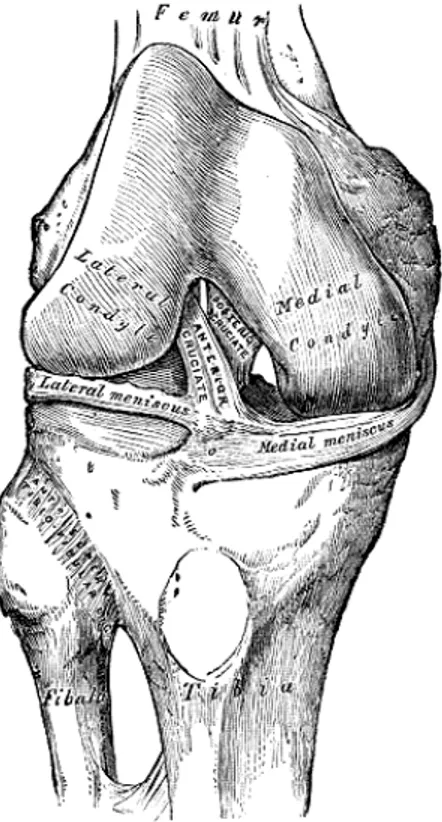
rotation (Ex/In). The rotation about the floating axis is designated as ab/adduction (Ab/Ad). FEMUR TIBIA ANTERIOR CRUCIAT LIGAMENT LATERAL MENISCUS QUADRICEPS TENDON FIBULAR COLLATERAL LIGAMENT PATELLAR LIGAMENT PATELLA ARTICULAR SURFACE FIBULA
1.2 Anatomy, Morphology, and Mechanics
The human knee is a unique tri-articular joint responsible for the most demanding biomechanical functions of our musculoskeletal system (Figure 1.3). The three distinct contact surfaces are the patello-femoral joint and the medial and lateral femoral articulations. Although the tibio-femoral articulations involve only two bones, the distal tibio-femoral condyles and tibial plateaus articulate in as separate but coordinated manner. These joint movements are further regulated and stabilized dynamically by muscle contractions, and passively by ligamentous and capsular tension. The major part of the detailed description of the human knee anatomy which follows is taken from the Gray’s anatomy book (Gray, 1918).
i
BonesThe femur is the longest and strongest bone in the skeleton. The femur, like other long bones, is divisible into a body (diaphysis) and two extremities (epiphyses). The diaphysis is almost perfectly cylindrical in most of its extent. In the erect posture, it is not vertical, but it inclines gradually downward and medialward, so as to approach the lower part of the contro-lateral femur, with the purpose of bringing the two knee joints near to the line of gravity of the body. This inclination is necessary because the two proximal femurs are separated by a considerable interval, which corresponds to the breadth of the pelvis. Thus, the degree of this inclination varies among subjects, and it is larger in female than in male, on account of the greater breadth of the pelvis. The lower epiphysis, larger than the upper one, is somewhat cuboid in form, but its transverse diameter is larger than its antero-posterior: it consists of two oblong eminences known as the condyles (Figure 1.4). The articular surface of the lower end of the femur occupies the anterior, inferior, and posterior surfaces of the condyles. Its front part is named the patellar surface and articulates with the patella. It presents a median groove which extends downward to the intercondylar fossa and two convexities, the lateral of which is broader, more prominent, and extends farther upward than the medial. The lower and posterior parts of the articular surface constitute the tibial surfaces for articulation with the corresponding condyles of the tibia and menisci.
Figure 1.4: Lower extremity of right femur viewed from below (Gray, 1918).
Figure 1.5: Upper surface of right tibia viewed from above (Gray, 1918). The tibia is situated at the medial side of the leg, and, excepting the femur, is the longest bone of the skeleton. It is prismoid in form, expanded above contracted in the lower third, and again enlarged but to a lesser extent below. In male, its direction is vertical, and parallel with the bone of the opposite side, but in the female it has a slightly oblique direction downward and lateralward, to compensate for the greater obliquity of the femur. It has a body and two extremities. The upper extremity is large, and expanded into two eminences, the medial and lateral condyles (Figure 1.5). The superior
articular surface presents two smooth articular facets. The medial facet,
oval in shape, is slightly concave in the frontal, and in the sagittal plane. The lateral, nearly circular, is concave in the frontal plane, but slightly convex in the sagittal plane, especially at its posterior part, where it is prolonged on to the posterior surface for a short distance. The central portions of these facets
articulate with the condyles of the femur, while their peripheral portions support the menisci of the knee-joint, which here intervene between the two bones.
The patella is a flat, triangular bone, situated on the front of the knee-joint (Figure 1.3 and Figure 1.6). It is usually regarded as a sesamoid bone (i.e. a bone embedded within a tendon), developed in the tendon of the Quadriceps femoris, and resembles these bones (1) in being developed in a tendon; (2) in its center of ossification presenting a knotty or tuberculated outline; (3) in being composed mainly of dense cancellous tissue. The primary functional role of the patella is knee extension. In fact, the patella increases the leverage of the Quadriceps femoris muscle group by increasing the angle at which it acts.
ii
Joints, Ligaments and MenisciThe bones of the skeleton are joined to one another at different parts of their surfaces, and such connections are termed Joints or Articulations. The articulations of the human body are divided into three classes: synarthroses or immovable, amphiarthroses or slightly movable, and diarthroses or freely movable. Where the joints are immovable, as in the articulations between all the bones of the skull, the adjacent margins of the bones are almost in contact, being separated merely by a thin layer of fibrous membrane, named the sutural ligament. In certain regions at the base of the skull this fibrous membrane is replaced by a layer of cartilage. Where slight movement combined with great strength is required, the osseous surfaces are united by tough and elastic fibrocartilages, as in the joints between the vertebral bodies, and in the interpubic articulation. In the freely movable joints the surfaces are completely separated, the bones forming the articulation are expanded for greater convenience of mutual connection, covered by cartilage and enveloped by capsules of fibrous tissue. The cells lining the interior of the fibrous capsule form an imperfect membrane - the
synovial membrane - which secretes a lubricating fluid. The joints are
strengthened (i.e. restraining unphysiological movements) by strong fibrous bands called ligaments, which extend between the bones forming the joint. This latter class includes the greater number of the joints in the body such as
the interphalangeal joints, the joint between the humerus and ulna or the ankle and hip joints.
The knee joint was formerly described as a hinge-joint, but is really of a much more complicated character. It must be regarded as consisting of three articulations in one: two diarthroidal condyloid joints, one between each condyle of the femur and the corresponding meniscus and condyle of the tibia, and a third between the patella and the femur, partly arthrodial, but not completely so, since the articular surfaces are not mutually adapted to each other, so that the movement is not a simple gliding one. The bones of the knee joint are connected together by the following structures.
Figure 1.6: Right knee-joint. Anterior view (Gray, 1918).
The Articular Capsule (capsula articularis; capsular ligament) (Figure 1.6). The articular capsule consists of a thin, but strong, fibrous membrane which is strengthened in almost its entire extent by bands inseparably connected with it. Above and in front, beneath the tendon of the Quadriceps
strengthening bands are derived from the fascia lata and from the tendons surrounding the joint.
Figure 1.7: Right knee-joint, from the front, showing interior ligaments (Gray, 1918).
The Patellar Ligament (anterior ligament) (Figure 1.6). The patella ligament is the central portion of the common tendon of the Quadriceps femoris, which is continued from the patella to the tuberosity of the tibia. It is a strong, flat, ligamentous band, about 8 cm. in length, attached, above, to the apex and adjoining margins of the patella and the rough depression on its posterior surface, below, to the tuberosity of the tibia. Its superficial fibers are continuous over the front of the patella with those of the tendon of the Quadriceps femoris. The medial and lateral portions of the tendon of the Quadriceps pass down on either side of the patella, to be inserted into the upper extremity of the tibia on either side of the tuberosity.
medial collateral is a broad, flat, membranous band, situated nearer to the back than to the front of the joint. It is attached, above, to the medial condyle of the femur immediately below the adductor tubercle, below, to the medial condyle and medial surface of the body of the tibia. The Lateral Collateral
Ligament (LCL, ligamentum collaterale fibulare; fibular collateral
ligament) (Figure 1.8). The lateral collateral is a strong, rounded, fibrous cord, attached, above, to the back part of the lateral condyle of the femur, immediately above the groove for the tendon of the Popliteus, below, to the lateral side of the head of the fibula, in front of the styloid process.
Figure 1.8: Left knee-joint from behind, showing interior ligaments (Gray, 1918).
The Cruciate Ligaments (ligamenta cruciata genu; crucial ligaments). The cruciate ligaments are of considerable strength, situated in the middle of the joint, nearer to its posterior than to its anterior surface. They are called cruciate because they cross each other somewhat like the lines of the letter X, and have received the names anterior and posterior, from the position of
their attachments to the tibia. The Anterior Cruciate Ligament (ACL, ligamentum cruciatum anterius; external crucial ligament) (Figure 1.7) is attached to the depression in front of the intercondyloid eminence of the tibia, being blended with the anterior extremity of the lateral meniscus, it passes upward, backward, and lateralward, and is fixed into the medial and back part of the lateral condyle of the femur. The Posterior Cruciate
Ligament (PCL, ligamentum cruciatum posterius; internal crucial ligament)
(Figure 1.8) is stronger, but shorter and less oblique in its direction, than the anterior. It is attached to the posterior intercondyloid fossa of the tibia, and to the posterior extremity of the lateral meniscus, and passes upward, forward, and medialward, to be fixed into the lateral and front part of the medial condyle of the femur.
The Menisci (semilunar fibrocartilages) (Figure 1.9). The menisci are two crescentic lamellæ, which serve to deepen the surfaces of the head of the tibia for articulation with the condyles of the femur and to distributing the compressive loads from the femur to the tibia. The peripheral border of each meniscus is thick, convex, and attached to the inside of the capsule of the joint, the opposite border is thin, concave, and free. The upper surfaces of the menisci are concave, and in contact with the condyles of the femur, their lower surfaces are flat, and rest upon the head of the tibia, both surfaces are smooth, and invested by synovial membrane. Each meniscus covers approximately the peripheral two-thirds of the corresponding articular surface of the tibia. The medial meniscus (meniscus medialis; internal semilunar fibrocartilage) is nearly semicircular in form, a little elongated from before backward, and broader behind than in front. Its anterior end, thin and pointed, is attached to the anterior intercondyloid fossa of the tibia, in front of the ACL. Its posterior end is fixed to the posterior intercondyloid fossa of the tibia, between the attachments of the lateral meniscus and the PCL. The lateral meniscus (meniscus lateralis; external semilunar fibrocartilage) is nearly circular and covers a larger portion of the articular surface than the medial one. It is grooved laterally for the tendon of the Popliteus, which separates it from the fibular collateral ligament. Its anterior end is attached in front of the intercondyloid eminence of the tibia, lateral to, and behind, the ACL, with which it blends. The posterior end is attached behind the intercondyloid eminence of the tibia and in front of the posterior
is twisted on itself so that its free margin looks backward and upward, its anterior end resting on a sloping shelf of bone on the front of the lateral process of the intercondyloid eminence.
Synovial Membrane. The synovial membrane of the knee-joint is the
largest and most extensive in the body. Commencing at the upper border of the patella, it forms a large cul-de-sac beneath the Quadriceps femoris on the lower part of the front of the femur, and frequently communicates with a bursa interposed between the tendon and the front of the femur.
Figure 1.9: Head of right tibia seen from above, showing menisci and attachments of ligaments (Gray, 1918).
iii
Structure and Mechanics of Knee LigamentsAs seen, ligaments, lying internal or external to the joint capsule, bind bone to bone and supply passive support and guidance to joints. They function to supplement active stabilizers (i.e. muscles) and bony geometry (Akeson et al., 1984). Well suited for their functional roles, ligaments offer early and increasing resistance to tensile loading over a narrow range of joint motion. This allows joints to move easily within normal limits while causing increased resistance to movement outside this normal range.
Ligaments and tendons are collagenous tissues with their primary building unit being the tropocollagen molecule (Viidik, 1973). Tropocollagen molecules are organized into long crossstriated fibrils that are arranged into bundles to form fibres. Fibres are further grouped into bundles
called fascicles which group together to form the ligament (Figure 1.10). Collagen fibre bundles are arranged in the direction of functional need and act in conjunction with elastic and reticular fibres along with ground substance, which is a composition of glycosaminoglycans and tissue fluid, to give ligaments their mechanical characteristics. In unstressed ligaments, collagen fibres take on a sinusoidal pattern. This pattern is referred to as a "crimp" pattern and is believed to be created by the cross-linking or binding of collagen fibres with elastic and reticular fibres.
Figure 1.10: Schematic diagram of the hierarchic structure of ligament. The whole ligament is composed of fibre bundles even more small up to reach the basic structural element, which is the tropocollagen molecule.
From a mechanical point of view, ligaments are composite, anisotropic structures exhibiting non-linear time and history-dependent viscoelastic properties. The structural properties of isolated tendons, ligaments, and bone-ligament-bone preparations are normally determined via tensile tests. In such tests, a ligament, tendon, or bone-ligament-bone complex is subjected to a tensile load applied at constant rate. A typical force-elongation curve obtained from a tensile test of bone-ligament-bone preparation is shown in Figure 1.11. The force-elongation curve is initially upwardly concave, but the slope becomes nearly linear in the pre-failure phase of tensile loading. The force-elongation curve represents structural properties of
the ligament. That is, the shape of the curve depends on the geometry of the specimen tested (e.g. tissue length and cross-sectional area).
Figure 1.11: Example of a force-elongation curve obtained from bone-ligament-bone specimen. Four regions are commonly used to describe a force-elongation or stress-strain curve. Region 1 is termed the "toe region" and elicits a non-linear increase in load as the tissue elongates. Region 2 represents the linear region of the curve. In Region 3, isolated collagen fibres are disrupted and begin to fail. In Region 4, the ligament completely ruptures.
The material properties of the ligament are expressed in terms of a stress-strain relationship. Stress is commonly defined as the force divided by the original specimen cross-sectional area. Whereas, strain is defined as the change in length of the specimen relative to its initial length, divided by its initial length. Hence, a tissue's material properties may be obtained from force-elongation data by dividing the recorded force by the original cross-sectional area to give stress, and by dividing the difference between the specimen length and its original length by its original length to give strain. The advantage of constructing a stress-strain diagram is that to a first approximation the stress-strain behaviour is independent of the tissue
dimensions. Stress-strain or force-elongation curves are typically described in terms of four regions. These four regions are illustrated in Figure 1.11. Region 1 is referred to as the "toe region". The non-linear response observed in this region is due to the straightening of the "crimp" pattern resulting in successive recruitment of ligament fibres as they reach their straightened condition (Abrahams, 1967; Diamant et al., 1972). As the strain increases, the "crimp" pattern is lost and further deformation stretches the collagen fibres themselves (Region 2). As the strain is further increased, microstructural damage occurs (Region 3). Further stretching causes progressive fibre disruption and ultimately complete ligament rupture or bony avulsion at an insertion site (Region 4). A hypothetical curve relating the "crimp" pattern and collagen fibre stretch to various portions of a stress-strain curve is illustrated in Figure 1.12
Figure 1.12: Example of stress-strain curve to describe the relationship between changes in the collagen "crimp" pattern, or stretch, and ligament mechanical properties. An increasing of the strain in the ligament at the "toe region" of the curve produces a straightening of the "crimp" pattern. During the linear portion of the curve, the collagen fibres are stretched more and more with the increasing of the strain. As the ligament is further strained isolated ligament fibres begin to rupture and if deformation continues, then complete ligament fail occurs. Modified from (Butler et al., 1978).
Clinically, it is important to know the normal operating conditions of ligaments acting within the body. Such information is needed to relate isolated ligament-bone test data to that of ligaments acting in-vivo. A hypothetical force-elongation curve for the human ACL, as postulated by Noyes et al. (1984), is shown in Figure 1.13. Levels of daily activity are shown along the right vertical axis and hypothetical loading levels for the ACL on the left vertical axis. This curve suggests that during daily activities (such as walking or light jogging) the ACL operates along the "toe region" of the force-elongation curve. It is believed that ligaments are not generally loaded above one-fourth of their ultimate tensile load during these daily activities. The early part of Region 2 is considered the upper operating range of the ACL during strenuous activities as might be experienced during fast cutting or pivoting while running. Loading of the ACL beyond Region 2 results in ligament damage and may be incurred during events like clipping in football, a ski accident, or an incorrect landing during a gymnastics floor exercise.
Figure 1.13: A hypothetical force-elongation curve for a human ACL-bone complex is illustrated along with daily activities that correspond to specific loading levels. During routine daily activities such as walking and standing, ligaments are loaded to less than one fourth their ultimate tensile load. During strenuous activities such as fast cutting during intense running, loading levels may enter into region 3 where isolated fibre damage takes place. Modified from (Noyes et al., 1984).
iv
MusclesSkeletal muscles actuate the bones of the body to produce movements at the joints and provide stability by resisting movement across joints. Muscles are active structures which contract themselves, reducing length and providing force, when they are activated by the central nervous system. When standing erect in the attitude of “attention,” the weight of the body falls in front of a line carried across the centres of the knee-joints, and therefore tends to produce overextension of the articulations. This, however, is passively prevented by the tension of the anterior cruciate, oblique popliteal, and collateral ligaments. Nevertheless, the equilibrium of a subject is not provided only by passive structures. In fact, the nervous system controls the balance of the subject recruiting muscles with the capability to produce an opposite movement in order to recover the position of equilibrium.
At knee joint, muscles which produce flexion are called ‘Flexors’, whereas muscles which produce extension are called ‘Extensor’. The Extensor muscles are also defined ‘Antagonist’ of the Flexor ones, and viceversa. Thus, the nervous system can produce motion of the knee joint along different axes, such as flexion-extension and intra-extra axial rotation, controlling the recruitment and the activation of several muscles at the same time. Moreover, the nervous system can also increase the stability of the knee joint, restraining the joint movements due to external loads, by means of the contraction of both Agonist and Antagonist muscles at the same time.
Muscle is composed of many subunits and complex structural arrangements (Figure 1.14). Whole muscle is surrounded by a strong sheath called the epimysium. The gross muscle is divided into a variable number of subunits called fasciculi. Each fasciculus is surrounded by a connective tissue sheath called the perimysium. Fascicles may be further divided into bundles of fibres (or muscle cells) which are surrounded by a sheath called the endomysium (Fung, 1981; Ishikawa, 1983).
The orientation of fibres relative to the orientation of the whole muscle varies among different muscles. Regarding the fibre arrangement, muscle may be classified as fusiform, unipennate, bipennate, triangular, and strap. Fibres attach at both ends to tendon or other connective tissue.
Figure 1.14: Schematic representation of the organizational structure of muscle. The gross muscle is composed of bundles of fascicles that consist of groups of fibres. Fibres can be further divided into myofibrils that contain the myofilaments making up the sarcomeres.
Muscle fibres are multinucleated cells with the nuclei generally located along the cell periphery. The population density of nuclei is estimated to be 50-100 per millimetre of fibre length (Ishikawa, 1983). Muscles have a rich supply of blood vessels. Capillary networks are arranged around each fibre with the capillary density varying around different fibres types (Ishikawa, 1983). A motor unit consists of a single motoneuron and all the fibres it innervates. The number of fibres per motor unit is variable, ranging from just a few in ocular muscles, requiring fine control, to thousands in large limb muscles (Ishikawa, 1983). In intact whole muscle, motor units intermingle throughout the entire muscle cross-sectional area.
Extension of the leg on the thigh is performed by the Quadriceps femoris (Quadriceps extensor) (Figure 1.15, a). It is subdivided into separate portions, which have received distinctive names. One occupying the middle of the thigh, and connected above with the ilium, is called from its straight course the Rectus femoris. The Rectus femoris (Figure 1.15, a) is situated in the middle of the front of the thigh, it is fusiform in shape. It arises by two tendons: one, the anterior or straight, from the anterior inferior iliac spine, the other, the posterior or reflected, from a groove above the brim of the acetabulum. The muscle ends in a broad and thick aponeurosis which occupies the lower two-thirds of its posterior surface, and, gradually becoming narrowed into a flattened tendon, is inserted into the base of the patella. Flexion of the leg is performed by the Biceps femoris, Semitendinosus, and Semimembranosus, assisted by the Gracilis, Sartorius, Gastrocnemius, Popliteus, and Plantaris. The Biceps femoris (Biceps) (Figure 1.15, b) is situated on the posterior and lateral aspect of the thigh. It has two heads of origin: one, the long head, arises from the lower and inner impression on the back part of the tuberosity of the ischium, the other, the short head, arises from the lateral lip of the linea aspera, extending up almost as high as the insertion of the Glutæus maximus. The Gastrocnemius (Figure 1.15, d) is the most superficial muscle, and forms the greater part of the calf. It arises by two heads, which are connected to the condyles of the femur by strong, flat tendons. Both heads, also, arise from the subjacent part of the capsule of the knee.
External rotation is effected by the Biceps femoris, and internal rotation by the Popliteus, Semitendinosus, and, to a slight extent, the
a) b)
c) d)
Figure 1.15: Anterior (a, c ) and posterior (b, d) views of muscles of a right leg. The thigh is shown in (a, b) and the shank in (c, d) (Gray, 1918).
action especially at the commencement of the movement of flexion of the knee, by its contraction the leg is rotated inward, or, if the tibia be fixed, the thigh is rotated outward, and the knee-joint is unlocked. The Glutæus
medius (Figure 1.15, b) is a broad, thick, radiating muscle, situated on the
outer surface of the pelvis. It arises from the outer surface of the ilium between the iliac crest and posterior gluteal line above, and the anterior gluteal line below, it also arises from the gluteal aponeurosis covering its outer surface. It performs the abduction and the rotation inward/outward of the thigh together with other muscles. The Tibialis anterior (Tibialis anticus) (Figure 1.15, c) is situated on the lateral side of the tibia, it is thick and fleshy above, tendinous below. It arises from the lateral condyle and upper half or two-thirds of the lateral surface of the body of the tibia, from the adjoining part of the interosseous membrane. The fibres run vertically downward, and end in a tendon, which is apparent on the anterior surface of the muscle at the lower third of the leg. After passing through the most medial compartments of the transverse and cruciate crural ligaments, it is inserted into the medial and under surface of the first cuneiform bone, and the base of the first metatarsal bone. It performs the dorsiflexion of the foot together with other muscles.
1.3 Biomechanics: functional anatomy
Human knee joint provides two apparently contrasting functions: it must be mobile to achieve a large and smooth range of motion, and must be stable to guarantee strong support in activity. The knee joint must allow both flexion and axial rotation to occur while still maintaining stability. The tibio-femoral joint defines the kinematics of flexion, extension and axial rotation while the patello-femoral joint increases the efficiency of the extensor mechanism by enlarging the quadriceps lever arm.
i
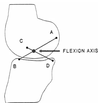
MobilityIn 1836, Weber (Weber and Weber) described knee motion as a combination of rolling, sliding, and axial rotation of the tibio-femoral joint (Muller, 1938). Nevertheless, as yet there have been few three-dimensional (3D) models described in the literature which incorporate this axial rotation with the rolling and sliding of the joint (Wismans et al., 1980; Feikes, 1999; Wilson et al., 2000; Di Gregorio et al., 2007). At first, the kinematic principles of the knee have been reduced to a two-dimensional midsagittal plane model known as the “cruciate” linkage (Muller, 1938; Kapandji, 1970; Goodfellow and O'Connor, 1978; O'Connor et al., 1989; O'Connor et al., 1990). The four links of this linkage represent the ACL, the PCL, a tibial link between the tibial cruciate insertion sites and a femoral link between the femoral cruciate origin sites (Figure 1.16). If the femoral link is articulated about the fixed tibial link, a graphic representation of knee joint motion can be obtained. Kapandji (Kapandji, 1970) has concluded that “the shape of the femoral condyles are geometrically determined by the lengths of each of the cruciate ligaments, as well as by the ratio of their individual lengths and the arrangements of their insertions”. As the knee is flexed from full extension, the point of intersection of the ACL and PCL (i.e. the flexion axis) links moves posteriorly.
Figure 1.16: The cruciate linkage comprises four links: AB is the neutral fibre of the ACL, CD is the neutral fibre of the PCL, BD is the link between the tibial attachment sites, and CA designates the femoral insertion points. The flexion axis is the point of intersection at each instant between the links AB and CD. (Kapandji, 1970)
A two-dimensional model has been constructed for a situation in which the tibia rotated on a stationary femur and the femur rotated on a stationary tibia (Figure 1.17) (Muller, 1938; O'Connor et al., 1990; O'Connor et al., 1989). These curves developed by plotting the centres of rotation in each situation are called centroids. The tibial centroide approximates a straight line whereas the femoral centroide is elliptical. As the two bones move on each other, they undergo both rolling and sliding. It is obvious that the femur must slide forward on the tibia plateau during flexion (roll-back mechanism): a pure rolling motion would result in the femur falling off the back of the tibia as the knee flexed over 100°. During the early phase of flexion, rolling is the predominant motion (Figure 1.18, A; and Figure 1.19), while flexion continues, sliding tends to predominate (Figure 1.8, B; and Figure 1.19).
Figure 1.17: The cruciate linkage drawn by the computer with the tibial link fixed, (a) and (c), and with the femoral link fixed, (b) and (d). the relative positions of the links are the same in the pair of diagrams (a) and (b) for each of the corresponding three configurations and in (c) and (d) for each of the corresponding 30 configurations. In (a) and (c), the femoral attachments of the ligaments move on circular arcs about their tibial attachments, and in (b) and (d) the tibial attachments move on circular arcs about the femoral attachments. The curve marked “Tibial centroide” and “Femoral centroide” are the tracks of the flexion axis of the joint on the tibia and femur, respectively, and are drawn through the successive intersections of the cruciates. (O'Connor et al., 1990)
Axial rotation of the tibia relative to the femur is the result of the application of the ground reaction force, the rotation applied by the musculature, and the screw-home mechanism. The ligaments and capsular structures act as restraints to this rotation. The musculature of the lower limb serves both as a passive restraint against rotation and to provide the force to cause rotation.
A B
Figure 1.18: From 0 to 10-15°, the motion is predominantly rolling (A), from 10-15° to 140-160° sliding (B). (Kapandji, 1970)
Figure 1.19: The diagram shows the cruciate linkage in two neighboring positions with the corresponding femoral surface touching a flat tibial plateau at F and F’. F’’ is the point on the femoral surface which makes contact with F. The slip ration is the distance F’F’’ measured along the femur, divided by the distance FF’ measured along the tibia. The graphs show the variation with flexion angle for convex, flat and concave tibial plateaus. (O'Connor et al., 1990)
The screw-home mechanism (external rotation of the tibia on the femur) (Figure 1.20) occurs automatically as the knee is extended. In the sagittal plane, the radius of curvature of the medial plateau is different from the lateral plateau. The medial tibial plateau is concave superiorly and the lateral is convex. Therefore, the articulating surfaces of the tibio-femoral joint are not fully conforming. When viewed distally, the lateral femoral condyle is longer than the medial. The unequal lengths and radii of curvature of the two femoral condyles, the shape of the tibial plateaus, and the position of the four primary ligaments force the tibia to rotate externally with extension (Kapandji, 1970).
A B C
Figure 1.20: The screw-home mechanism: coupled internal rotation of 20° of the tibia on the femur during knee flexion (Kapandji, 1970).
Figure 1.21: Functioning of the menisci: Sliding movements between the femur and the concave upper surface of the menisci allow flexion and extension, sliding movements between the flattened undersurface of the meniscus and the tibial plateau allow rotation and anteroposterior translation of the tibia (Kapandji, 1970)
Lateral radiographs of the knee demonstrate that the articular surfaces of the tibia in the sagittal plane are virtually flat, articulating with the convex femoral condyles only at a point. This appearance is misleading. The dissimilar shapes of the articular surfaces of the two bones are made congruent by the interposed meniscus. The important function of the meniscus in distributing compressive load from the femur to the tibia was reported from direct measurements in human and porcine joints in the laboratory (Walker and Erkman, 1975; Shrive et al., 1978). The menisci are integral parts of the tibial articular surface, making it conform to the shape of the femoral condyle as the acetabulum conforms to the head of the femur. Sliding movements between the femur and the concave upper surface of the meniscus allow flexion and extension, sliding movements between the flattened undersurface of the meniscus and the tibial plateau allow rotation and anteroposterior translation of the tibia (Figure 1.21). In fact, sliding movements usually occur simultaneously at both the femoromeniscal and tibiomeniscal joints (Goodfellow and O'Connor, 1994).
ii
StabilityJoint Stability is provided by both intrinsic and extrinsic anatomical mechanisms. The intrinsic stability of the knee joint is provided by the four primary ligaments, the capsule, the shape of the bony structures, and the menisci. The ligaments act as tensile check reins which permit motion to occur within limits. The limits of motion are dependent on orientation of these ligaments. The ACL is the primary check against anterior displacement of the tibia relative to the femur, with the PCL being the primary stabilizer preventing posterior displacement. In knee flexion, the superficial MCL is the first defence against external rotation with the ACL acting as a secondary restraint. In knee extension, the ACL and superficial MCL act together as primary stabilizers against external rotation. With the knee flexed, internal rotation is prevented first by the cruciate ligaments and secondly by the LCL. In extension, the ACL is the primary stabilizer and the LCL the secondary (Marshall and Rubin, 1977). The primary and secondary knee stabilizers that resist valgus stresses (opening of the medial side of the knee) are the superficial MCL and the ACL respectively. Varus knee stresses