Mission synthesis of sine-on-random excitations for accelerated vibration qualification testing

(1)

ALMA MATER STUDIORUM

UNIVERSITÀ DI BOLOGNA

SCUOLA DI INGEGNERIA E ARCHITETTURA

–Sede di Forlì–

Corso di Laurea Magistrale in

INGEGNERIA MECCANICA

Classe LM-33

TESI FINALE DI LAUREA

in Crediti nel Settore Ing-Ind/13

Mission Synthesis of Sine-on-Random excitations for accelerated

vibration qualification testing

CANDIDATO

RELATORE

Andrea Angeli

Ing. Marco Troncossi

CORRELATORE

Ing. Bram Cornelis

Anno Accademico 2014/2015

Sessione III

(2)

2

Abstract

In most real-life environments, mechanical or electronic components are subjected to vibrations. Some of these components may have to pass qualification tests to verify that they can withstand the fatigue damage they will encounter during their operational life. In order to conduct a reliable test, the environmental excitations can be taken as a reference to synthesize the test profile: this procedure is referred to as “test tailoring”.

Due to cost and feasibility reasons, accelerated qualification tests are usually performed. In this case, the duration of the original excitation which acts on the component for its entire life-cycle, typically hundreds or thousands of hours, is reduced. In particular, the “Mission Synthesis” procedure lets to quantify the induced damage of the environmental vibration through two functions: the Fatigue Damage Spectrum (FDS) quantifies the fatigue damage, while the Maximum Response Spectrum (MRS) quantifies the maximum stress. Then, a new random Power Spectral Density (PSD) can be synthesized, with same amount of induced damage, but a specified duration in order to conduct accelerated tests.

In this work, the Mission Synthesis procedure is applied in the case of so-called Sine-on-Random vibrations, i.e. excitations composed of random vibrations superimposed on deterministic contributions, in the form of sine tones typically due to some rotating parts of the system (e.g. helicopters, engine-mounted components, …). In fact, a proper test tailoring should not only preserve the accumulated fatigue damage, but also the “nature” of the excitation (in this case the sinusoidal components superimposed on the random process) in order to obtain reliable results. The classic time-domain approach is taken as a reference for the comparison of different methods for the FDS calculation in presence of Sine-on-Random vibrations. Then, a methodology to compute a Random specification based on a mission FDS is presented. In case of Sine-on-Random environments, it will better represent the original excitation than a purely random specification.

(3)

3

Sommario

In molte applicazioni, i componenti meccanici o elettronici sono soggetti a vibrazioni. Alcuni di questi componenti potrebbero dover essere sottoposti a prove di qualifica a vibrazione, per verificare che possano resistere al danno a fatica che incontreranno nel corso della loro vita operativa. Al fine di condurre una validazione appropriata, le eccitazioni reali possono essere prese come modello per sintetizzare il profilo vibratorio del test di qualifica: questa procedura prende il nome di “test tailoring”.

Per ragioni di costi e fattibilità, di solito sono eseguiti test di qualifica accelerati. In questo caso, la durata dell’eccitazione originale che sollecita il componente per tutto il suo ciclo vita, tipicamente centinaia o migliaia di ore, è ridotta. In particolare, la procedura di “Mission Synthesis” permette di quantificare il danno indotto dalla vibrazione reale attraverso due funzioni: il Fatigue Damage Spectrum (FDS) quantifica il danno a fatica, mentre il Maximum Response Spectrum (MRS) quantifica il massimo stress. Quindi, può essere sintetizzata una nuova random Power Spectral Density (PSD) con la stessa quantità di danno indotto, ma una durata ridotta in modo da poter condurre test accelerati.

Nel lavoro seguente, la procedura di Mission Synthesis viene applicata nel caso delle cosiddette vibrazioni Sine-on-Random, ovvero eccitazioni composte da vibrazioni random sovrapposte a contributi deterministici, sotto forma di componenti sinusoidali causate tipicamente da parti rotanti del sistema (per esempio nel caso di elicotteri, componenti montati sul motore, ...). Infatti, un adeguato test tailoring dovrebbe preservare non solo il danno a fatica accumulato, ma anche la "natura" dell'eccitazione, in questo caso le componenti sinusoidali sovrapposte al segnale random, per ottenere risultati attendibili. L’approccio classico nel dominio del tempo viene preso come riferimento per il confronto di diversi metodi per il calcolo del FDS in presenza di vibrazioni Sine-on-Random. Quindi, viene presentato un metodo per la sintesi di un profilo Sine-on-Random partendo da un dato FDS di riferimento. In caso di ambienti sottoposti a vibrazioni Sine-on-Random, un profilo con la stessa tipologia rappresenterà meglio l’eccitazione originale rispetto a una specifica con caratteristiche puramente random.

(4)

4

Acknowledgements

I would like to express my gratitude to my supervisor at the University of Bologna and promoter of this project, Marco Troncossi, for his continued support and assistance before, during and after the development of my activity.

I would also like to offer special thanks to Bram Cornelis, my supervisor at LMS International, for his invaluable support and help, really fundamental to conduct my activity.

Thanks to my friends, because they know me and they are still my friends. Thanks to my family.

Thanks to everyone who has contributed, directly or indirectly, to this project. Thanks to C.

(5)

5

Introduction

Mechanical components, during their operational life, may be subjected to vibrations. These vibrations can induce fatigue damage, due to the repeated loading and unloading of the material, and the components must be designed to last through the induced damage. Therefore, to avoid the risk of rupture, the components can be validated with qualification tests. The real environmental excitations can be taken as a reference to make these tests as representative as possible: this procedure is called test tailoring. The problem is that usually the real vibrations cannot be used without manipulations due to time and cost reasons. A solution can be to quantify the damage induced by the environmental vibrations and then synthesize a new profile with a reduced duration but the same amount of damage.

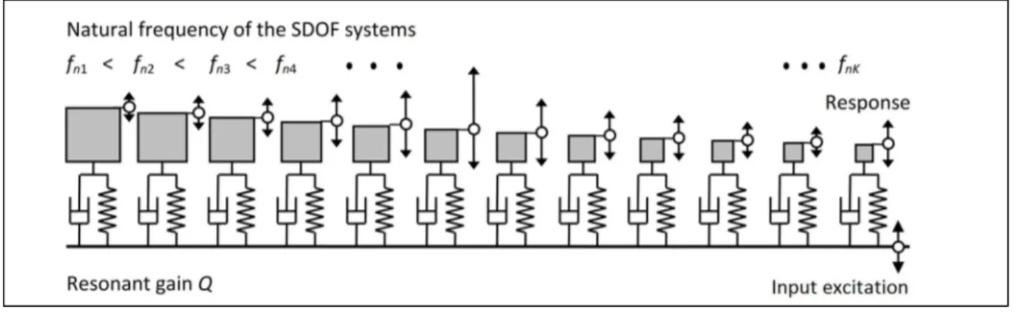
One of these approaches for the test tailoring is the Mission Synthesis. It represents the generic component with a series of linear Single Degree of Freedom (SDOF) systems, with a fixed damping ratio and the natural frequency that varies in the range of the component’s frequencies of interest. Then, the response of each SDOF system to the input (i.e. environmental) excitation is calculated. The response evaluation can be approached in the time domain, but in the case of very long signals, the calculations could have a too long duration. So, again for time and cost reasons, a frequency domain approach is usually preferred.

Once the SDOF response is calculated, the induced damage is quantified, under a number of approximations, by means of two functions. The Fatigue Damage Spectrum (FDS) quantifies the fatigue damage, while the Maximum Response Spectrum (MRS) quantifies the maximum stress. If the reason of the procedure is to preserve the fatigue damage, the original profile and the synthesized profile must have the same FDS. Usually, to avoid another type of damage, also the calculation of the new MRS is accomplished, in order to verify that the maximum induced stress will not pass the ultimate stress limit. Otherwise, if the purpose is the preservation of the shock damage, the new profile must have the same MRS of the real excitation.

It is generally assumed that the environmental vibration has random characteristics, that is the excitation has random values with a Gaussian probability distribution. Therefore, also the synthesized profile can be random, to preserve this property and make the test more realistic. However, in some special cases, the vibration does not follow a Gaussian distribution. In particular, if a rotating part is present, a so called “Sine-on-Random” vibration usually shows up (e.g. helicopters, engine-mounted components, …). The mechanical component is thus subjected to a random Gaussian excitation, superimposed to deterministic components, in the form of sinusoids, due to the rotor.

In order to perform accelerated tests, for feasibility and cost savings causes, a test profile which represents as much as possible the real environment but with a limited duration is needed. The purpose of this work is to investigate how to quantify the damage in presence of Sine-on-Random vibrations and, then, to find a way to synthesize a time reduced profile which preserves not only the fatigue damage but also the characteristics of the sinusoidal tones.

(7)

7

In [Chapter 1] a review of the Mission Synthesis procedure is presented.

In [Chapter 2] a model for the quantification of the damage with the classical time domain approach is introduced and validated in case of purely random vibrations. Therefore, it can be used as the reference in the following comparisons in presence of Sine-on-Random excitations. In [Chapter 3] different frequency domain methods for the damage calculation in case of Sine-on-Random vibrations are compared, with the aim to find the best one. Then, starting from the advantages of each method, a new procedure for the FDS calculation is proposed.

In [Chapter 4] a new method for the synthesis of a Sine-on-Random profile starting from a reference FDS is disclosed and its benefits over the synthesis procedure of a purely random profile are discussed.

(8)

8

Chapter 1 – Mission Synthesis

Almost all mechanical components are subjected to vibrational environments during their life cycle, and such environments have been shown to be damaging. Therefore, to reduce failure rates, it is essential to take these vibrational stresses into account at an early stage of the development of the components and to be able to design accurate tests to achieve this purpose. These tests must satisfy the following criteria:

- Be severe enough to ensure that, if the part survives the test, it can be safely assumed that it will do also in a real environment.

- Be sufficiently representative of the real environment to give enough confidence that if the unit fails during the test, it will fail also in real operating conditions.

Thus, a balance must be found between severity and accuracy. The test should give the developer the confidence that its severity guarantees to prevent failures that may occur under normal operating conditions, but at the same time it should avoid an overestimation of the damage that would lead to an expensive oversized component. So, the goal of the Mission Synthesis is to design the optimum test.

There are two main possible strategies to determine the test specifications:

- Testing in situ: this method consists in mounting the component to test on the source of vibrations and expose it to the actual working conditions. Such testing has obviously the advantage that it is highly representative of the real excitations. But in most cases due to cost, time and feasibility reasons it is highly impractical, if not impossible, to conduct that type of tests.

- Testing by simulation of conditions in a laboratory:

o Based on standards: using standard test specifications is useful when the component will be subjected to unknown conditions or in any case in which they are not easily measurable or assumable. However, standards are conservative by nature and, in general, they will lead to an overdesigned component, causing higher costs.

o Based on real environmental data: when the life cycle of the component is well known, a specification which closely simulates the real environment can be developed. In general, the risk of oversizing is diminished. On the other hand, the equipment will be designed for a specific life cycle. So, changes to the test specifications will require a new procedure. In addition, it is important that not only the specification respects the real environment but also that the actual testing does it.

In this scenario, the Mission Synthesis procedure lets to determine test specifications based on real environmental data [Ref. 1].

(9)

9

So, if the life cycle of the component is well acquainted, the first step is to break it down into a series of phases of known duration and loading conditions, called situations. Environmental data are necessary to evaluate each situation identified in the life cycle. In general, situations occur one after the other, in series, but parallel situations are also possible [Fig. 1.1].

Figure 1.1: Example of life profile of a component with situations in series/parallel

The determination of the simulated environment consists of three stages:

- The estimation of the equivalent damage potential of the real environment by the computation of the Maximum Response Spectrum (MRS) and Fatigue Damage Spectrum (FDS) functions.

- The possible application of a safety factor to consider all the uncertainties that are involved in the definition of the test specifications.

- The combination into one global test specification of all the individual situations and their equivalent damage potentials.

For the estimation of the equivalent damage potential by means of the FDS/MRS functions, a generic component is represented with a series of linear Single Degree of Freedom (SDOF) systems [Fig. 1.2], with a fixed damping ratio and the natural frequency that varies in the range of the component’s frequencies of interest. It will be shown that this simplification lets to reduce the problem of the damage quantification in finding the response of a linear SDOF system. Usually, the environmental vibration is given in the form of an acceleration and it corresponds to an excitation applied to the base of the system. Then, the elongation caused by the excitation can be calculated, in the form of the relative displacement response between the mass and the support of the SDOF system. The calculation can be done in the time or in the frequency domain.

(10)

10

Figure 1.2: the component is modeled as a series of SDOF systems

The Maximum Response Spectrum (MRS) is the maximum value of the relative displacement response over its duration, for each natural frequency of the SDOF system. Usually it is reported in the form of an acceleration, with a multiplication by the squared natural pulsation of the SDOF system. Due to the linearity of the system, if the material is linear, a linear relation between the maximum relative displacement and the stress peak inflicted to the system can be considered, so the MRS quantifies the maximum stress induced by the excitation and it is typically used to verify that it does not pass the ultimate stress limit of the material to avoid shock ruptures.

Calling a certain natural frequency of the SDOF system and the maximum value of the relative displacement response at that natural frequency, the MRS expression is:

= (2 ) ∙ ( ) [EQ. 1.1]

The Fatigue Damage Spectrum (FDS) function, instead, is used to quantify the fatigue damage caused by the excitation. In fact, after the calculation of the relative response displacement of the SDOF system, an estimation of the induced fatigue damage can be accomplished, thanks to some further assumptions:

- the fatigue relation Stress – Number of Cycles is described by the Basquin’s law: = where is the number of cycles to failure under stress of amplitude and and are constants characteristic of the material

- a linear relation exists between the maximum relative displacement and the peak stress inflicted to the system: = where is a constant of the material

- a method is used to count the peaks and the relative number of cycles (e.g. Rainflow Counting)

- the Miner’s linear accumulation rule for the damage is used: = ∑ where the total damage is given by the sum of the levels of damage .

Afterwards, an exponential proportionality between the fatigue damage and the relative displacement emerges and, at each frequency, the value of the FDS function is precisely this estimated fatigue damage. In particular:

(11)

11

= = = = ( ) = ( ) [EQ. 1.2]

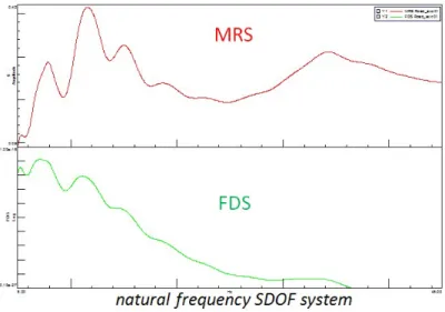
In the end, the FDS and MRS functions are usually represented by plotting the calculated values of the maximum response and the fatigue damage versus the natural frequency of the single degree-of-freedom linear system [Fig. 1.3]. The MRS and FDS expressions [EQ. 1.1], [EQ. 1.2] will be discussed in detail in [Chapter 2].

Figure 1.3: MRS, FDS examples

After their calculation and, if necessary, the application of the safety factor, the FDS and MRS functions for each situation have to be all combined in a single specification:

- Situations in parallel: in this case the equipment is subjected only to one of the parallel situations, so the combined specification is obtained by:

o The envelope of the MRSs o The envelope of the FDSs

- Situations in series, the combined effect will be:

o The envelope of the MRSs (to consider the higher peak stress) o The sum of the FDSs (to consider the cumulative fatigue damage)

Now, all the environmental situations are represented by a unique specification and the inflicted damage is fully described by its MRS and FDS functions. Then, accelerated qualification tests are usually preferred, for the purpose to keep them feasible and with limited costs. Thus, a new profile with a reduced time but the same amount of damage can be synthesized:

- In case the fatigue damage has to be preserved, the FDS of the new excitation has to be the same of the original one.

(12)

12

- In case the maximum stress has to be conserved, the MRS of the new profile has to be the same of the original one.

Also in the first case a check on the maximum stress of the synthesized excitation, represented by its MRS, has to be done in order to verify that the component to test will not incur in a different type of rupture, due to the passing of the ultimate stress limit.

The qualification test can now be carried out on the component in exam. Obviously, the better the test profile represents the environmental excitation, the more reliable the qualification test will be. Given that the Mission Synthesis method in case of Gaussian random vibrations is well known, it permits to synthesize a new test profile in the form of a Power Spectral Density (PSD) with the same induced damage of the environmental excitation but with a reduced duration, in order to perform accelerated qualification tests.

Thus, the aim of this work is to investigate the procedure in presence of the so called Sine-on-Random vibrations, sinusoidal contributions superimposed on a random excitation, looking for the best way to quantify the fatigue damage and, then, to synthesize a time reduced profile based on a target FDS that preserves as much as possible the characteristics (i.e. the deterministic components) of the original signal.

(13)

13

Chapter 2 – Random vibrations

The first step in the evaluation of different methods for the calculation of the damage inflicted by Sine-on-Random vibrations is to obtain a reference value for the comparison. This reference has been identified in the classical time domain approach for the calculation of the FDS and MRS. The idea is to compare the results with the frequency domain approach in the case of purely random vibrations and then, since the time domain model works with every timeseries, it can be used to compare the different frequency domain methods also in the case of Sine-on-Random excitations.

2.1. Time domain approach

Relative Displacement Response of a SDOF system

A generic component is modeled with a series of Single-Degree-of-Freedom (SDOF) systems, then the relative displacement response of each system to the excitation is calculated in the time domain and the response is eventually used to obtain the FDS and MRS functions. Therefore, the first passage in the procedure is the calculation of the relative displacement response of a SDOF system:

Figure 2.1: SDOF system

In [Fig. 2.1] ( ) is the displacement response of the system to the input displacement excitation ( ). It is worth noting that, in case of measured vibrations, the excitation is usually known in the form of acceleration ( ). Then, the relative displacement response is defined as:

(14)

14

( ) = ( ) − ( ) [EQ. 2.1]

The SDOF system is characterized by its parameters: mass , stiffness , and damping . So, it can be described by the natural frequency and the quality factor (or the damping ratio ):

= ₂1 [EQ. 2.2]

= _{2 =}1 √ [EQ. 2.3]

Given a SDOF system with fixed damping ratio and natural frequency, and the base acceleration input, the relative displacement response in the time domain is obtained with the Duhamel, or convolution, integral:

( ) = ℎ( − ) ( ) = − ( ) ( )sin ( − ) [EQ. 2.4]

Where ℎ( ) is the impulse response function of the system, is the natural pulsation and is the damped natural pulsation:

ℎ( ) = sin( ) [EQ. 2.5]

= 2 [EQ. 2.6]

= 1 − [EQ. 2.7]

There are different algorithms to compute the integral and calculate the relative displacement response, for example:

- The numerical integration of the Duhamel integral - The recursive filtering methods:

o Impulse invariant method (Kelly-Richman algorithm) o Ramp invariant method (Smallwood algorithm)

In fact, to avoid the numerical integration over the entire interval, a popular technique is to use a digital recursive filter to simulate the SDOF system and, using a sampled input, the output of the filter is assumed to be a gauge of the response. Being the input the measured environmental excitation, it is typically already given in a sampled form. Then, the recursive filtering approach consists in the calculation of the response ( + ), where is the sampling interval, with a

(15)

15

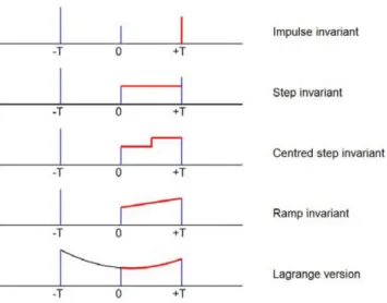
recursion formula using only the previous values of the response ( ) and the input signal in the time interval. Different approximations of the input [Fig. 2.2] in the interval [0, ] define different filter design methods. In particular, the impulse invariant method considers the input as an impulse at that instant, so the excitation is represented by a series of scaled impulses at each sampling time. But, at high values of the natural frequencies of the SDOF system, where high is related to the value of the sampling frequency of the input signal, this approximation leads to some errors, due to the possible interference of the impulse responses.

Figure 2.2: Different input approximations

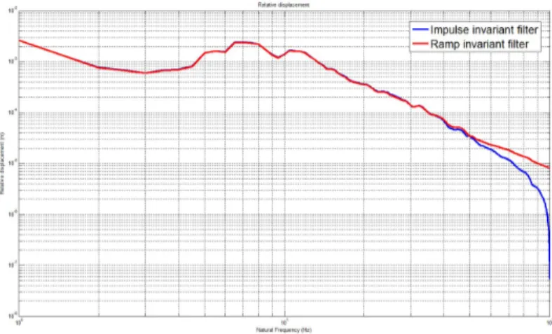
The problem has long been recognized [Ref. 2] and the ramp invariant method solves this issue approximating the input as a ramp between the instant of interest and the previous one. This leads, for the Smallwood algorithm, to better results also at high values of the natural frequencies [Fig. 2.3] and, for this reason, it was chosen in this work for the implementation.

The expressions of the ramp invariant filter ( ) and its coefficients are:

( ) = ₊+ ₊+ [EQ. 2.8] = −2 ( )_cos( ₎ _{[EQ. 2.9]} = ( ) _{[EQ. 2.10]} = 2 ( )_cos( _{) − 1 +} ( ) _{(2 − 1) sin(} _{) +} [EQ. 2.11] = −2 ( )_cos( _{) + 2 1 −} ( ) _{− 2} _{(2 − 1)} ( )_sin( ₎ [EQ. 2.12] = (2 + ) ( )₊ ( ) _{(2 − 1) sin(} _{) − 2 cos(} ₎ [EQ. 2.13]

(16)

16

So the response can be calculated with the following recursive formula, for each sample time :

= − − − − − [EQ. 2.14]

How to obtain the recursive filtering parameters, expressions [EQ. 2.8÷14], is detailed in [Ref. 2]. Given the modeling of the generic component as a series of SDOF systems, the procedure is repeated setting each frequency in the range of interest as natural frequency of the SDOF system and, then, calculating the response in the complete spectrum.

Figure 2.3: Relative displacement response – comparison between Impulse and Ramp invariant methods

Maximum Response Spectra (MRS)

Once the relative displacement response is calculated, the Maximum Response can be obtained taking the maximum value of the relative response displacement at a certain natural frequency, and multiplying it by the squared natural pulsation, to give the results in the form of acceleration:

= max ( ) [EQ. 2.15]

= (2 ) [EQ. 2.16]

Where ( ) is the calculated relative displacement response, is its maximum value and is the natural frequency of the SDOF system. Repeating the procedure for each natural frequency in the range of interest gives the complete MRS function [Fig. 2.4].

(17)

17

Figure 2.4: MRS calculation – comparison with Test.Lab

Fatigue Damage Spectra (FDS)

For the calculations of the FDS, once the Relative Displacement Response is obtained with the ramp invariant method, a peak counting algorithm is needed. The most popular one, due to his reliability, is the Rainflow Counting method, therefore it is the algorithm that has been chosen also in this work.

The algorithm basically consists in counting the cycles or the half-cycles of stress – time signals. In this case, the stress is represented by the relative displacement response of the SDOF. So, the result of the Rainflow Counting is the number of cycles of a certain magnitude of the relative displacement response peaks. The name rainflow comes from a comparison between the method and the flow of a rain falling on a pagoda. In fact, the procedure can be schematized as:

- Reduce the time history to a sequence of peaks and troughs.

- Imagine the time history as pagoda: rotate the figure, putting the starting time at the top. - Each peak is imagined as a source of water that falls down the pagoda.

- Count the number of half-cycles by looking for terminations in the flow occurring when either:

o It reaches the end of the time history

o It merges with a flow that started at an earlier peak or, in case of trough, it encounters a trough of greater magnitude

- Repeat the previous step for the troughs.

- Assign a magnitude to each half-cycle equal to the stress difference between its start and termination.

- Pair up the half-cycles of identical magnitude to count the number of complete cycles. Typically, there are some residual half-cycles.

Given the many different ways to implement the algorithm, it has been chosen to use the one described in the ASTM standard [Ref. 3]. After the calculations, it is possible to represent the result in a histogram with the number of cycles associated with each magnitude [Fig. 2.5].

(18)

18

Figure 2.5: Rainflow Counting histogram

Then, if the material is linear and given the linearity of the SDOF system, a linear relation exists between the relative displacement peaks and the stress peaks:

= [EQ. 2.17]

ℎ = ℎ

So, the number of cycles at a certain stress amplitude inflicted to the system is known. If the Stress-Number of cycle (S–N) curve of the material follows the Basquin’s law:

= [EQ. 2.18]

Where is the number of cycles to failure of the material under a stress of amplitude and and are constants characteristic of the material (in the literature their values are usually given for a test bar under sinusoidal stress). It has to be noted that, in the Rainflow Counting, the magnitude associated with each (entire or half) cycle can be referred to the range or the amplitude, with:

= ( − )

= ( − )/2

The choice does not influence the procedure, except for the parameters of the Basquin’s law [EQ. 2.18] that correlate the number of cycles to rupture at a certain stress. Given that in the S–N

(19)

19

curve [Fig. 2.6] the literature typically refers the stress to the amplitude, for coherence in this work the relative displacement amplitude has been taken as magnitude.

Figure 2.6: S-N curve

Then, knowing that the damage inflicted to the system by the application of one cycle of a certain stress is:

= 1 = [EQ. 2.19]

In the case of cycles of stress , the associated damage will be:

= = = [EQ. 2.20]

Now, given levels of damage induced by likewise peak amplitudes each one achieved in cycles, the total damage can be calculated considering the Miner’s linear rule of accumulation [Ref. 4]:

= [EQ. 2.21]

(20)

20

= = = ( ) = ( ) [EQ. 2.22]

Repeating the calculation of the fatigue damage, assigning each value in the range of interest to the natural frequency of the SDOF, leads to the complete FDS function [Fig. 2.7].

Figure 2.7: FDS calculation – comparison with Test.Lab

2.2. Frequency domain approach

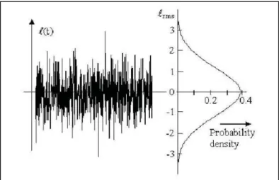
In the case of the frequency domain, if the random excitation has a Gaussian probability distribution of its values [Fig. 2.8], a statistical approach can be used. The procedure can be summarized as:

- Calculation of the Power Spectral Density (PSD) of the vibratory excitation.

- Calculation of the root mean squared (rms) values , , of the relative displacement, velocity and acceleration of the response of the SDOF system to the input PSD.

- Calculation of the mean frequency and the mean number of peaks per unit time. - Calculation of the irregularity factor of the response.

(21)

21

Figure 2.8: Probability density function (Gaussian) of instantaneous values of a random signal

Calculation of the response, peaks distribution

Assuming that the PSD of the excitation is available [Fig. 2.9], the first step is the calculation of the SDOF system response. Knowing the transfer function of the SDOF system ( ):

( ) = 1

(2 ) 1 − ₊ [EQ. 2.23]

Ref.

It is possible to calculate the rms values of the relative displacement, velocity and acceleration responses due to the input PSD with the expressions [Ref. 5]:

= _{4 ∙ (2 )}Q ∙ ( ) [EQ. 2.24]

= (2 ) _{[EQ. 2.25]}

= (2 ) _{[EQ. 2.26]}

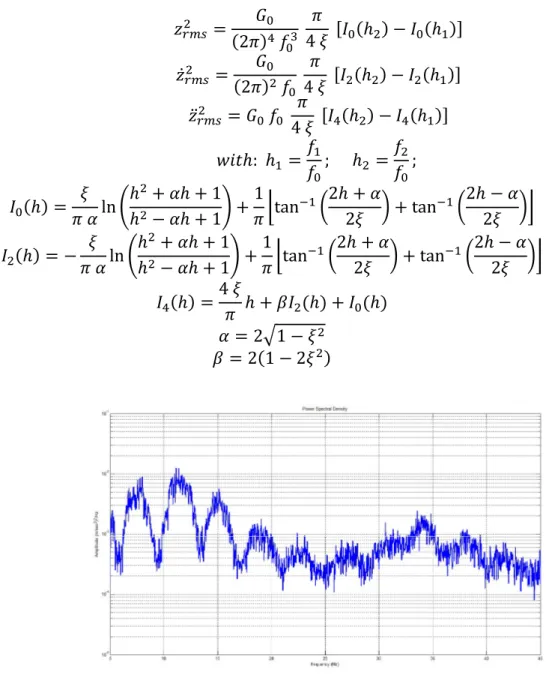
Where , , are the rms values of the relative displacement, velocity and acceleration responses to the PSD of amplitude . The expressions are obtained in case of white noise, but they give a good approximation also if the noise is not white, when the quality factor is rather high (the case of interest, narrow band scenario). Otherwise, the expressions for , , in case of a constant PSD between two frequencies are given in [Ref. 5]:

(22)

22 = (2 ) 4 (ℎ )− (ℎ ) [EQ. 2.27] = (2 ) 4 (ℎ ) − (ℎ ) [EQ. 2.28] = 4 (ℎ ) − (ℎ ) [EQ. 2.29] ℎ: ℎ = ; ℎ = ; (ℎ) = ln ℎ + ℎ + 1ℎ − ℎ + 1 +1 tan 2ℎ +2 + tan 2ℎ −2 (ℎ) = − ln ℎ + ℎ + 1ℎ − ℎ + 1 +1 tan 2ℎ +2 + tan 2ℎ −2 (ℎ) =4 ℎ + (ℎ) + (ℎ) = 2 1 − = 2(1 − 2 )

Figure 2.9: Random vibration – Power Spectral Density

Then, the expressions for the mean number of zero crossing per unit time with positive slope and the mean number of positive maxima per unit time of the response are [Ref. 6]:

=₂1 [EQ. 2.30]

=₂1 [EQ. 2.31]

Consequently, the irregularity factor of the response can be defined as the ratio of the average number of zero crossings per unit time with positive slope to the average number of positive maxima per unit time [Ref. 5]:

(23)

23

= [EQ. 2.32]

Following its definition, the parameter r is a measure of the width of the response. In fact, for a broad band process, the number of maxima is much higher than the number of zeros, tending to the limiting case where = 0. While in the case of a narrow band signal, the number of passages through zero is equal to the number of peaks, until the limiting case where = 1.

Since the narrow band scenario follows the case of the response to a SDOF system of rather high quality factor (or low damping ratio ), the second is the case of interest. In this case it is known that the probability density of the response peaks tends to the Rayleigh’s law [Fig. 2.10] [Ref. 6]:

= [EQ. 2.33]

Figure 2.10: Rayleigh probability density function

Fatigue Damage Spectra (FDS)

Thus, if the signal is stationary and Gaussian, it is possible to avoid the time-consuming direct peaks counting of the time domain approach. The probability density of the peaks in the response can be used instead. Precisely, if the probability to find the peak is known, the distribution of the fatigue cycles for the stress , comparable to a Rainflow Counting histogram, can be calculated using the equation:

(24)

24

Where is the duration. So, in a similar manner as the previous chapter [EQ. 2.20], the caused damage due to the stress is:

= = [EQ. 2.35]

Where is the number of cycles to failure under a stress . And, following the Miner’s rule [EQ. 2.21], it is possible to find the expression of the expected fatigue damage due to every stress

:

= ( )_{( )} [EQ. 2.36]

Now, applying the linear displacement – stress relation [EQ. 2.17] and the Basquin law [EQ. 2.18] leads to:

= [EQ. 2.37]

Then, the substitution of the found probability density of the peaks [EQ. 2.30] gives the expression for the FDS calculation:

= = [EQ. 2.38]

In this particular case, the following version is obtainable [Ref. 5]:

= = √2 _{Γ 1 + 2} [EQ. 2.39]

(25)

25

Where Γ is the gamma function. This expression is exact for perfectly narrow band responses ( = 1) but it has been shown [Ref. 5] that it gives a good approximation for > 0.567. It is used for the FDS calculation in [Fig. 2.11].

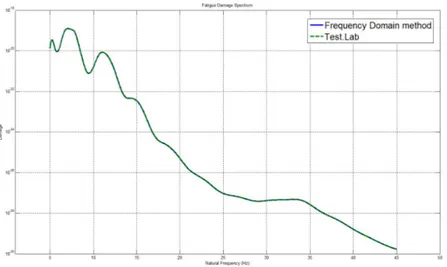
Figure 2.11: FDS calculation – comparison with Test.Lab

Maximum Response Spectra (MRS)

For the MRS calculation, from [EQ. 2.34] and knowing that a linear displacement – stress relation exists [EQ. 2.17]:

= [EQ. 2.40]

Assuming that the largest peak , over the duration , will be passed only once:

( ) = 1 [EQ. 2.41]

Thus, [EQ. 2.40] can be rewritten for the largest peak :

( ) = 1 [EQ. 2.42]

Given that the expression of the peaks distribution [EQ. 2.33] is known, the value of that satisfies the relation [EQ. 2.42] can be found iteratively.

(26)

26

= (2 ) [EQ. 2.43]

Otherwise, the simplified relation can be obtained [Ref. 1]:

= (2 ) 2 ln( ) [EQ. 2.44]

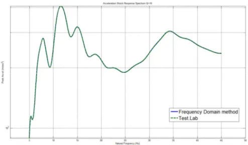
This expression is used for the MRS calculation in [Fig. 2.12].

Figure 2.12: MRS calculation – comparison with Test.Lab

A detailed discussion and the way to obtain the expressions for the probability distribution of the peaks and the FDS and MRS functions calculation [EQ. 2.33], [EQ. 2.39], [EQ. 2.44] are given in [Ref. 5], [Ref. 6].

2.3. Discussion

Both the methods implemented in MATLAB scripts show a very good correspondence with their respective LMS Test.Lab calculations. As a further validation, the time domain approach can be compared directly with the frequency domain approach in case of purely random vibrations. Thus, the MRS and FDS functions are computed for the same excitation, in the form of timeseries and corresponding PSD, with the two different methods.

(27)

27

Figure 2.13: FDS calculation – Time/Frequency domain comparison

Figure 2.14: MRS calculation – Time/Frequency domain comparison

In the case of the FDS calculation [Fig. 2.13], a very good correspondence in the fatigue damage estimation is shown, due to the good prediction of the peaks distribution of the frequency domain method. In [Fig. 2.14], instead, a not perfect correspondence emerges in the case of the MRS calculation. Considering that it takes into account only the maximum value of the response, a similar result was expected due to the statistical approximation of the frequency domain method. Therefore, given the match of the damage quantification between the time and the frequency domain approaches, the time domain model can be taken as the reference to compare the different frequency approaches also in presence of Sine-on-Random vibrations, for which equations shown in [Chapter 2.2] cannot be used.

(28)

28

Chapter 3 – Sine-on-Random vibrations

Many structural components in dynamic environments may experience both sinusoidal and random loadings at the same time. In fact, if a rotating part is present, its unbalancing typically generates a periodic excitation, in addition to the random noise produced by the rest of the environment. Therefore, a so called Sine-on-Random vibration is present: it is an excitation made of a deterministic contribution (i.e. sinusoidal tones), superimposed on a random signal.

An excitation of this kind can be represented with a PSD for the random part, plus the superimposed sinusoids in the form of accelerations at their own frequencies [Fig. 3.1].

Figure 3.1: Example Sine-on-Random profile

In order to calculate the induced damage, the method described in [Chapter 2.2] cannot be used. In fact, due to the presence of the sine tones, the Gaussian distribution of the signal is modified. This leads to a peaks distribution different from the case of purely random signals (Rayleigh distribution).

Thus, in this chapter, different approaches for the evaluation of the fatigue damage in the case of these Sine-on-Random profiles are compared, investigating the pros and cons of each one:

 Time domain approach: after obtaining a timeseries of the excitation, if not already available, the method described in [Chapter 2.1] can be used.

 Frequency domain approach:

o Sine-on-Random with “sufficiently spaced sinusoids”: in the particular case of a single sinusoid superimposed on a random signal, Rice [Ref. 7] found the probability density function of the envelope of the composed excitation. It can be used to

(29)

29

determine the peaks distribution, so a statistical approach for the damage calculation can be accomplished. An extension for multiple sinusoids is proposed by Lalanne [Ref. 1]: if the frequencies of the sine tones are sufficiently spaced, each sinusoid can be considered independently.

o Sine-on-Random with “not sufficiently spaced sinusoids”: the extension of the Rice probability density function in case of multiple sinusoids [Ref. 7] has to be numerically integrated to find the peaks distribution of the combined excitation. Then, the statistical approach for the damage calculation can be carried out.

o “Mixed approach”: the advantages of the two previous methods are summed up. The closed form expression for the sufficiently spaced sinusoids is normally utilized, while the numerical integration is computed only when necessary to avoid an underestimation of the damage.

As said, the need of a different method from the time domain approach is due to the long time necessary for the calculations in the case of very long signals. Nevertheless, due to its reliability, it is taken as the reference to compare the damage estimation of the frequency domain methods.

3.1. Sufficiently spaced sinusoids

Case of a single sinusoid

In a first instance, the simple case of a single sinusoid superimposed on a random excitation is considered. The signal can be written as:

( ) = (2 + ) + ( ) [EQ. 3.1]

Where , and are the amplitude, frequency ad phase of the sinusoid and ( ) is the random noise. In the case of a measured environmental vibration, the amplitude of ( ) is typically an acceleration.

The idea is to apply a statistical procedure similar to the frequency domain method in case of purely random vibrations. The difference is that, due to the presence of the sinusoid, in this situation the excitation does not follow a Gaussian distribution [Fig. 3.2], so the Rayleigh distribution cannot be used to estimate the peaks. The new peaks distribution has to be found, instead.

(30)

30

Figure 3.2: (single) Sine-on-Random signal and probability density distribution of instantaneous values

Calculation of the response, peaks distribution

The first step of the procedure is the calculation of the relative displacement response. In this case, the SDOF system can be considered subjected to the sinusoidal component and to the random part separately. For the calculation of the response to the random part, assuming it is given in the form of a PSD, the expressions [EQ. 2.24÷26] of [Chapter 2.2] are recalled:

= _{4 ∙ (2 )}Q ∙ ( ) = (2 ) z = (2 )

Where , , are the rms values of the relative displacement, velocity and acceleration responses to the random PSD of amplitude .

The response to the sinusoidal excitation is still a sinusoid, thus, its amplitude is equal to the maximum displacement response and it is given by the amplitude of the excitation and the known transfer function of the system.

= (2 ) 1 − ₊ [EQ. 3.2] = √2 [EQ. 3.3] = (2 ) _{[EQ. 3.4]} = (2 ) _{[EQ. 3.5]}

Where is the maximum value of the relative displacement response to the sinusoidal excitation. Consequently, , , are the rms values of the relative displacement, velocity and

(31)

31

acceleration responses to the sinusoidal excitation. The sine amplitude is considered an acceleration.

Thus, the rms values of the total displacement, velocity and acceleration responses , , have to take into account both the random and the sinusoidal signals. They are given by the expressions [Ref. 1]:

= + _{[EQ. 3.6]}

= + [EQ. 3.7]

= + [EQ. 3.8]

The mean number of zero crossing per unit time and the mean number of peaks per unit time are consequently modified [Ref. 1]:

= ₂1 [EQ. 3.9]

= ₂1 [EQ. 3.10]

Then, defining ( ) as the envelope of , a Sine-on-Random signal of the kind [EQ. 3.1], the probability distribution function of this envelope has been deducted by Rice [Ref. 7]:

P( ) = ∙ [EQ. 3.11]

with: ( ) = ₂ _{( !)}1

Where is the rms value of the random noise and is the Bessel function of the first kind of order zero.

(32)

32

Figure 3.3: Probability density function of the envelope of a (single sinusoid) Sine-on-Random signal

It is known [Ref. 8] that the probability density function of the envelope is the same of the peaks amplitude. Due to the linearity of the SDOF system, the response to a Sine-on-Random excitation has still the Sine-on-Random characteristics, thus [EQ. 3.11] can be used to estimate the peaks distribution of the response:

= ( ) = ∙ [EQ. 3.12]

Where is the peak amplitude of the response. So, it is possible to follow the same procedure of the statistical approach for purely random vibrations, but using the new probability distribution.

Fatigue Damage Spectra (FDS)

In the same way as the frequency approach for random vibrations [EQ 2.34], the peaks distribution can be used to estimate the Rainflow Counting:

= [EQ. 3.13]

Where is the duration and is the number of estimated cycle at the displacement amplitude .

(33)

33

= [EQ. 3.14]

After the substitution of the peaks distribution [EQ. 3.2], the expression for the fatigue damage becomes:

= ∙ [EQ. 3.15]

In this particular case of a single sinusoid, the integral above [EQ. 3.14] has a closed form solution [Ref. 8]:

= = √2 _{Γ 1 + 2} _{− 2,1,−} [EQ. 3.16]

ℎ: = [EQ. 3.17]

(∝, δ, x) = (∝) ( )_{( ) !} Where is referred as the hypergeometric function.

Maximum Response Spectra (MRS)

For the MRS calculation, a recursive research for the highest peak as in [Chapter 2.2] is possible. From expression [EQ. 3.13] assuming that the largest peak , over the duration , will be passed only once:

( ) = 1 [EQ. 3.18]

( ) = 1 [EQ. 3.19]

And knowing the expression for the peaks distribution [EQ. 3.12], the value of that satisfies the relation [EQ. 3.19] can be found iteratively. Thus, the MRS expression is:

(34)

34

Otherwise an approximated expression for the MRS calculation can be obtained [Ref. 1]:

= (2 ) 2 ln [EQ. 3.21]

In case:

> ~ 1000 ℎ: = ₂1

Where is solely the mean frequency of the random vibration as calculated in [Chapter 2.2], the following expression gives a better approximation [Ref. 1]:

= (2 ) √2 + 2 ln( ) [EQ. 3.22]

(35)

35

Figure 3.5: MRS calculation in case of single sinusoid – comparison with Test.Lab

The expressions [EQ. 3.16], [EQ. 3.12] are applied to the MRS and FDS calculations in [Fig. 3.4], [Fig. 3.5]. Their derivation is given in [Ref. 1].

Multiple “sufficiently spaced” sinusoids extension

Obtained the expressions for a single sine tone superimposed on a random signal, a first approach in case of multiple ( ) sinusoids was proposed by Lalanne [Ref. 1]. If the frequencies of the sine tones are sufficiently spaced, only the nearest sinusoid to the natural frequency of the SDOF system has relevance on the damage, while the others are negligible. This is due to the expression of the maximum relative response to a sinusoidal excitation: it assumes its greatest value in case of resonance (the sine tone frequency equals the system natural frequency), and it decreases going away from that frequency [Fig. 3.6].

(36)

36

In this particular case, the sinusoids can be considered independently, so after the calculations of the separate FDS functions of each sine tone plus the random noise, the complete spectrum is given by their envelope. The same procedure is applicable to the MRS.

= , , … , _{[EQ. 3.23]}

= , , … , _{[EQ. 3.24]}

The method is applied in [Fig. 3.7] for the FDS calculation and in [Fig. 3.8] for the MRS calculation.

(37)

37

Figure 3.8: MRS calculation - Spaced sinusoids method vs. Time domain approach

3.2. Not sufficiently spaced sinusoids

In the case the frequencies of the sinusoids are closer, the damage contribution of the other sine tones is not negligible. Therefore, the damage between the frequencies of two not sufficiently spaced sinusoids is influenced by both the sine tones and the previous method, which considers only one sinusoid at a time, will give an underestimation of the fatigue damage [Fig. 3.9].

(38)

38

In this case, a new statistical approach that takes into account all the sinusoids at the same time is necessary [Ref. 9]. In case of several sine tones superimposed on a random noise, the signal can be written as:

( ) = ( ) + (2 + ) [EQ. 3.25]

Where , , are the amplitudes, frequencies ad phases of the sinusoids and ( ) is the random noise.

Calculation of the response, peaks distribution

Again, due to the linearity of the SDOF system, the response has the same characteristics of the excitation. So, in case of an input of the kind [EQ. 3.25], if the PSD of the random part and the acceleration amplitudes of the sinusoids are known, the responses can be obtained with the expressions of the previous chapter [EQ. 2.24÷26], [EQ. 3.2÷3.5]:

= _{4 ∙ (2 )}Q ∙ ( ) = (2 ) z = (2 ) = (2 ) 1 − ₊ = √2 = 2 = 2

Where, again, is the response to the random part and is the response to the – ℎ sinusoid. In this case the rms values of the total relative displacement, velocity and acceleration responses

(39)

39

= + [EQ. 3.26]

= + [EQ. 3.27]

= + [EQ. 3.28]

The consequently modified mean number of peaks of the response per unit time is:

= ₂1 [EQ. 3.29]

If ( ) is the envelope of ( ), a Sine-on-Random signal as defined in [EQ. 3.25], the probability density function of has been obtained by Rice [Ref. 7]:

( ) = ( ) ∗ ( ) [EQ. 3.30]

Where is the rms value of ( ) and is the Bessel function of the first kind of order zero. The formula [EQ. 3.30] assumes that the random signal and the sinusoids are independent random variables, thus the sine frequencies have to be incommensurable.

Again, knowing that the probability distribution of the envelope is the same of the peaks [Ref. 8], and that, due to the linearity of the SDOF system, the response to a Sine-on-Random excitation has still Sine-on-Random characteristics, [EQ. 3.30] can be used to estimate the peaks distribution of the response:

= ( ) = ∗ [EQ. 3.31]

Where is the peak amplitude of the response taking into account all the sine tones. The effectiveness of the formula [EQ. 3.31] has been tested, verifying its accuracy in the prediction of the peaks distribution even in case of not respected assumptions, considering that typically the sinusoids of a Sine-on-Random vibration have multiple frequencies.

(40)

40

Fatigue Damage Spectra (FDS)

As seen in case of purely random vibration [EQ. 2.34] or a single Sine-on-Random signal [EQ. 3.13], the estimated number of cycles for a certain relative displacement amplitude, is given by:

= [EQ. 3.32]

Where is the duration.

Knowing the peaks distribution [EQ. 3.31], a comparison between the result of the Rainflow Counting in the time domain and the expected number of cycles from [EQ. 3.32] is possible [Fig. 3.10].

Figure 3.10: Rainflow Counting comparison with the predicted distribution

Also in the worst case, when the assumptions of the Rice formula are not fully respected (i.e. multiple frequencies) and when the response is not perfectly narrowband, it still gives a good approximation of the number of cycles, well describing the distribution in the tale where the induced damage is higher.

Then, with the same procedure in case of single sinusoid but the new probability density function [EQ. 3.31] and mean number of peaks [EQ. 3.29], the FDS expression can be derived:

(41)

41

The substitution of the expression of the peak distribution gives:

= = [EQ. 3.34]

Unfortunately, in this case a closed form solution is not obtainable. How to properly set the parameters for a numerical integration is shown in [Appendix A].

Figure 3.11: FDS calculation in case of not spaced sinusoids – comparison of the different methods

Thus, the expression [EQ. 3.34] solves the problem of the fatigue damage underestimation in case of not sufficiently spaced sinusoids [Fig. 3.11], but at the price of a numerical integration.

3.3. “Mixed approach”

The advantage of the first presented method is that a closed form expression for the fatigue damage calculation is obtainable. Unfortunately, it gives an underestimation of the damage in case of sinusoids with closer frequencies. This issue is solved by the second method, but two numerical integrations are needed. Then, the optimal solution can be the utilization of the closed form expression, with the implementation of the numerical integrations only when necessary, to avoid an excessive underestimation of the damage.

(42)

42

To decide when the numerical integrations are needed, a criterion has to be defined. From the previous chapters, it is known that there is an exponential relation between the fatigue damage and the relative displacement z:

= ∝ z

Now, the expressions for the calculations of the rms values of the total relative displacement response with the two different methods are recalled. In particular, in case of sufficiently spaced sinusoids, its expression considers only the highest sinusoidal response [EQ 3.8]:

= +

While in case of not sufficiently spaced sinusoids, all the sine responses are taken into account. Thus, the expression is [EQ 3.23]:

= +

So, after the calculation of the SDOF responses with the two different methods, it is possible to estimate the underestimation of the “method 1” and decide if the implementation of the “method 2” is necessary:

= (1 − )

1 − > ( ) →

(43)

43

3.4. Discussion

A closed form expression for the damage estimation in case of a single sine tone superimposed on a random vibration has been shown. Its application even in presence of multiple sinusoids is possible in case of sufficiently spaced frequency: only one sinusoidal response can be considered at a time (the closer to resonance), while the others are negligible.

Unfortunately, if the sine tones are not spaced, this method gives an underestimation of the fatigue damage. In fact, the other sine tones are not effectively negligible in that case.

The solution is the utilization of the probability density function of multiple sinusoids superimposed on a random signal. The new expression for the fatigue damage calculation solves the problem of the underestimation, but it requires two numerical integrations.

Thus, a “mixed” approach is proposed. It starts from the closed form formula to compute the damage. Then, if necessary, it corrects the underestimation computing the numerical integrations of the second method. It combines a proper damage estimation with a not excessive computational load.

Its application is shown in figure [Fig. 3.12].

(44)

44

Chapter 4 – Test profile synthesis

If a critical mechanical or electronic component will be subjected to a Sine-on-Random excitation during its operational life, a qualification test may be necessary to verify its endurance with respect to the induced fatigue damage. In order to conduct a qualification test, a new specification profile has to be synthesized. In particular, this profile has to be based on the real environment to be realistic, but at the same time its duration has to be limited for the test feasibility.

Assuming that the fatigue damage has to be preserved, the Fatigue Damage Spectrum of a certain excitation has been calculated (with one of the described methods) and then it will be used as the mission FDS to synthesize a new profile with the same damage but a reduced duration.

Some authors [Ref. 10], [Ref. 11] have suggested different methods in order to transform the amplitude of the sinusoids into narrowband PSDs and add them to the random part, therefore a new complete PSD is obtained. Nevertheless, a procedure to synthesize a real Sine-on-Random profile is still missing.

In this chapter, a new method for the synthesis of a Sine-on-Random profile is compared with the standard random Power Spectral Density (PSD) profile synthesis:

 Synthesis of a Random PSD profile: previously, a way to compute the Fatigue Damage Spectrum from a random Gaussian PSD was shown. By inverting the procedure, but varying the duration, it is possible to obtain a time reduced PSD profile from a mission FDS. This is the standard procedure for the profile synthesis.

 Synthesis of a Sine-on-Random profile: if the original excitation has the Sine-on-Random characteristics, a similar synthesized profile will be more advisable. Starting from the expression for the FDS calculation of a (single sinusoid) Sine-on-Random excitation described in [Chapter 3.1], it is possible to obtain a procedure for a Sine-on-Random profile synthesis. A parameter which represents the ratio between the amplitude of the sinusoids and the random part in the original environmental data is needed.

4.1. Random Power Spectral Density profile synthesis

It follows the method described in [Chapter 2.2]. Starting from a reference FDS and inverting the procedure, a purely random PSD is synthesized. A reduced duration will give a higher amplitude of the profile, but the same amount of damage.

The expressions [EQ. 2.24], [EQ. 2.39] for the computation of the rms value of the relative response displacement for an input PSD of amplitude and of the relative calculation are recalled:

(45)

45

= _{4 ∙ (2 )}Q ∙ ( )

= = √2 _{Γ 1 + 2}

Knowing that the mean number of zero crossing per unit time corresponds to the mean frequency of the signal and, in case of narrowband response, it can be set equal to the natural frequency of the SDOF system [Ref. 12]:

= [EQ. 4.1]

It is possible to obtain the PSD amplitude of the synthesized profile for a specified duration ′:

( ) =4 ∙ (2 ) = 4 ∙ (2 ) ∙ ( ) ′ √2 Γ 1 + 2

[EQ. 4.2]

In case of purely random vibrations, if the environmental excitation is given in the form of a PSD, the Mission Synthesis procedure of FDS calculation and PSD synthesis with reduced time is straightforward:

=

Where , are the amplitude and duration of the original PSD and , are the amplitude and duration of the synthesized PSD.

The parameters , have no influence, due to their simplification in the procedure (FDS calculation and specification synthesis). The Basquin coefficient , instead, affects the value of the synthesized PSD and its choice, from the literature or an experimental research, has relevance. It is already clear that this method is not optimum in case of Sine-on-Random excitations because it only aims at matching the fatigue damage, whereas the nature of the excitation is not considered: the synthesized profile has purely random characteristics and the deterministic part (i.e. the sinusoids) is not preserved.

(46)

46

4.2. Sine-on-Random profile synthesis

As seen in [Chapter 3.1] the fatigue damage in case of a single sinusoid superimposed on a random excitation can be calculated from [EQ. 3.16]:

= = √2 _{Γ 1 + 2} _{− 2,1,−}

ℎ: =

Considering the already seen expressions [EQ. 2.24÷26], [EQ. 3.3÷8] for the responses: = √2 = (2 ) = (2 ) = (2 ) = (2 ) = + = +

The mean number of peaks per second can be rewritten in function of the parameter:

= ₂1 = ₂1 +

+ =

+

+ [EQ. 4.3]

Thus, if , the ratio between the sine and the random amplitudes of the response, is known or obtainable, it is possible to invert the procedure and obtain a synthesized Sine-on-Random profile with a specified duration ′. In particular, the first passage is to obtain the responses given by the new profile:

′ =

′ √2 Γ 1 + 2 − 2,1,−

(47)

47

′ = ∙ ′ [EQ. 4.5]

Where ′ is the relative response displacement induced by the new random PSD and ′ is the relative response displacement induced by the new sinusoid. The duration ′ can be set at the desired value for the synthesized profile.

Now, recalling the expressions [EQ. 2.24], [EQ. 3.2]:

= _{4 ∙ (2 )}Q ∙ ( ) =

(2 ) 1 − ₊

They can be inverted and the amplitudes of the sinusoid ′ and of the random PSD ′ of the new profile can be obtained:

′( ) =4 ∙ (2 ) ∙ ′ [EQ. 4.6]

= (2 ) ∙ 1 − _{+ ∙ ′} [EQ. 4.7]

And the synthesized (single sinusoid) Sine-on-Random profile is obtained.

In case of several sinusoids superimposed on the random vibration, if the sine frequencies are sufficiently spaced, as seen in [Chapter 3.1] a similar extension is applicable: each sine tone is treated independently. The procedure can be schematized as:

- Considering a single sine tone superimposed on the random part, the method above is applied in order to obtain the synthesized Sine-on-Random profile.

- The procedure is repeated for each sinusoid.

- Then, only the minimum value for the random part between the different ones is taken [Fig. 4.1].

- The complete Sine-on-Random specification is composed by all the synthesized sinusoids and the “minimum” random signal.

(48)

48

Figure 4.1: Synthesis random component

In [Chapter 3.1] it has been shown that, if the sine tones are close, the FDS formula gives an underestimation of the damage due to the not negligible sinusoids. In the synthesis procedure, if the starting mission FDS is properly calculated (without damage underestimation), the procedure will overestimate the random part between the frequencies of the close sinusoids. In fact, considering only one sine tone at a time, the residual damage due to the neglected sinusoids (taken in account by the mission FDS but not by the synthesis formula) will be added to the random excitation, leading to a more severe synthesized profile. If the severity overestimation is seen as a further safety factor of the procedure, the error is acceptable.

4.3. Discussion

The advantage of the synthesis of a Sine-on-Random profile over a purely random PSD is that it does not simply attempt to match the reference FDS but it also better describes the peaks distribution of the original signal. As seen, in fact, the maxima of a Sine-on-Random excitation do not follow a Rayleigh distribution as in the case of the purely random vibrations.

Recalling the expression of the FDS [EQ. 1.2]:

(49)

49

It can be noticed that an exponential relation between the fatigue damage and the relative displacement peaks is present, with the Basquin coefficient as exponent. So, if the peaks distribution is well described by the synthesized excitation, the dependence on the accurate knowledge of the b coefficient during the mission synthesis procedure is reduced. Since this coefficient is usually taken from the literature, given the difficulty in the estimation due to its dependence on the material and the type of the excitation [Ref. 13], it is frequently a source of possible errors.

Consequently, it is clear that in case of Sine-on-Random environment, if a Sine-on-Random synthesized profile is less subjected to errors due to a possibly inaccurate choice of the b coefficient, it gives a strong advantage over the standard purely random profile synthesis.

4.4. Application example: helicopter data

Starting from real environmental data with Sine-on-Random properties, the two different synthesis methods are applied. The utilized data [Fig. 4.2] were measured on a helicopter whose rotor has the following characteristics:

 Fundamental frequency at 392 rpm (~ 6.53 ).  Blade passage at 32.65 Hz (five blades).

Figure 4.2: Sine-on-Random timeseries

Starting from the measured timeseries, the time domain approach of [Chapter 2.1] is applied for the FDS calculation [Fig. 4.3].

(50)

50

Figure 4.3: FDS from timeseries

Then, a PSD [Fig. 4.4] is synthesized with the method described in [Chapter 4.1].

Figure 4.4: random PSD synthesis

For the synthesis of a Sine-on-Random profile, instead, a relation between the original sine tone and the random excitation is needed before proceeding. Since the measured environmental data are in the form of a single timeseries (sum of the sinusoidal and random parts), some manipulations are necessary. The following procedure is followed:

(51)

51

- By knowing the fundamental frequency of the rotor, it is possible to extract the harmonic component from the signal (the “harmonic filtering” function implemented in Test.Lab has been used)

- The Fourier transform is applied to the extracted harmonic component, in order to find the amplitudes and the phases of the fundamental sinusoid and its harmonics.

- The residual part is the random component and the relative PSD is obtained.

- The sinusoids and the random excitations are applied to the SDOF system, in order to obtain the values rms values of the relative displacement responses [EQ. 2.24], [EQ. 3.2]. Therefore, the parameter is obtainable and the synthesis is possible. The extracted phases of the sinusoids are kept in the new profile, to preserve as much as possible the characteristics of the original excitation. In this case, the fundamental sinusoid and its 14 superior harmonics are considered [Fig. 4.5].

Figure 4.5: Sine-on-Random profile synthesis

In order to evaluate the two different methods, in a first instance, the duration of the synthesized profiles is taken equal to the original measured vibration. Then, a comparison between the original FDS and the FDSs of the synthesized profiles is carried out [Fig. 4.6]. In particular, a timeseries is derived from the synthesized profiles and the time domain approach is used, for the purpose of a comparison as much reliable as possible.

(52)

52

Figure 4.6: FDS comparison - Original profile, Sine-on-Random synthesis, Random synthesis (b=5)

During the Mission Synthesis procedure, the following value of the b coefficient, typical in case of electronic components [Ref. 13], has been used:

= 5

Now, if it is assumed that the real value of the b coefficient was different, the actual FDSs of the original signal and the synthesized profiles can be computed and compared. The examples with = 7 [Fig. 4.7], = 12 [Fig. 4.8] and = 3 [Fig. 4.9] show that, as assumed, the Sine-on-Random synthesis is more representative of the original environment. In fact, while the recalculated FDS of the Sine-on-Random profile is still close to the original FDS, the FDS of the random profile shows a distance from the reference. In particular, the example with = 3 is particularly significant. It highlights the possible severity underestimation of the purely random signal that will lead to an improperly qualification test.

(53)

53

(54)

54

Thus, in case the synthesized specification has the same duration as the original signal, it is confirmed that the synthesized Sine-on-Random profile is less sensitive to a possible not perfect knowledge of the Basquin coefficient b, compared to a purely random synthesis. The reason relies on the better representation of the peaks distribution of the Sine-on-Random profile. In fact, if a comparison between the Rainflow Counting of the original signal and the expected distributions with the Rayleigh (purely random synthesis) and Rice (Sine-on-Random synthesis) probability functions is shown [Fig. 4.10], it can be noticed that the Sine-on-Random specification is far more accurate in the peaks reconstruction.