Computational Fluid Dynamics analysis of heat transfer problems in heated channels with water at supercritical pressure

(1)

Università di Pisa

Facoltà di Ingegneria

Corso di Laurea Specialistica in Ingegneria Energetica

Computational Fluid Dynamics analysis of

heat transfer problems in heated channels with

water at supercritical pressure

Relatori

Prof. Ing. Walter Ambrosini

Em. Prof. J. Derek. Jackson

Dr. Shuisheng He

Dott. Ing. Nicola Forgione

Prof. Ing. Paolo Di Marco

Candidato

Marco Mucci

(2)

(3)

25 Settembre 2003 ⋯ 23 Aprile 2010 “A volte uno si crede incompleto

ed è soltanto giovane.” Italo Calvino

“Ogni volta che scopriamo nuove tecniche

spesso ci atteniamo stupidamente alle vecchie forme.” Pier Luigi Nervi

(4)

(5)

I

Abstract

The present work, partly carried out during a three month stage at the University of Aberdeen (UK), is aimed to investigate the heat transfer problem in heated channels with water at supercritical pressure. The analysis is performed with three different Computational Fluid Dynamics codes (SWIRL, an ―in-house‖ CFD code, FLUENT and STAR-CCM+, general-purpose CFD codes). The aim of this work is to evaluate the performances of different low-Reynolds number turbulence models in predicting mixed convection heat transfer of fluids at supercritical pressure, with particular attention to the features that are affected by the modifications of the turbulence field due to influence of flow acceleration and buoyancy.

Several simulations are performed and the predicted results are compared with the data obtained by the experimental facility in the Nuclear Engineering Laboratory at the University of Manchester. The simulated test section is 2 m long, with a diameter of 25.4 mm (1‖). Different operating conditions are imposed for water at 25 MPa, in both downward and upward flow.

Mainly, the analysis is conducted using the Yang-Shih turbulence model and the SWIRL CFD code in simple two-dimensional geometry. Results on a broad-spectrum of boundary conditions are achieved and a better understanding of the heat transfer behaviour was developed by the analysis of the dimensionless velocity and the dimensionless turbulent kinetic energy, for different axial locations along the pipe. Deterioration and enhancement phenomena are pointed out considering the ratio between the Nusselt number in the mixed convection flow and the Nusselt number of forced flow, while the effects of buoyancy are indicated by the Buoyancy parameter Bo*, introduced by Jackson, et al. (1979).

Some numerical aspects are also studied. The low-Reynolds number k-𝜀 turbulence models adopted in the work, are generally able to predict both heat transfer enhancement and deterioration phenomena even if, in some upward flow cases, wall temperature over prediction was obtained from the simulations, due to the large change in fluid properties when temperature reaches the pseudo-critical value. So, the predicted effect of buoyancy is much greater than suggested by a buoyancy parameter based on bulk temperature. Buoyancy and the consequent laminarization effects are the main reasons for the occurrence of deterioration in the considered experimental data, but other mechanisms also contribute to the occurrence of this phenomenon.

(6)

(7)

III

Acknowledgments

This thesis is the result of several months of intense research in direct contact with personalities involved in the project, whose contribution, in assorted ways to the research and the making of the thesis, deserve special mention.

First of all, this work would not have been possible without my family and “i Pisani”.

After this, I would like to express my deep and sincere gratitude to Prof. Walter Ambrosini, his understanding, encouraging and personal guidance have provided a good basis for the present thesis. I wish to express my warm and sincere thanks to Dr. Shuisheng He, whose advises gave me important guidance during my first steps at University of Aberdeen. For the same reasons, I am grateful to Prof. J. Derek Jackson for his important and effective support throughout this work although there have been few opportunities to meet together.

I wish to thank Dr. Nicola Forgione and Prof. Paolo Di Marco for their guidance on review and Dr. Medhat Sharabi that has provided assistance in numerous ways. Thanks also to the Cd-Adapco for the technical support provided and to the Università di Pisa and, in particular, to the Dipartimento di Ingegneria Meccanica, Nucleare e della Produzione, for the financial support, in the frame of to the International Academic Cooperation 2009-2010 between the Universities of Pisa, Manchester and Aberdeen.

(8)

(9)

V

List of Figures

Figure 1: Schematic P-T diagram ... 5

Figure 2: Water density trends (Sharabi, 2008) ... 6

Figure 3: Water specific heat trends as a function of Temperature (Sharabi, 2008) ... 7

Figure 4: Water specific heat as a function of Pressure (Sharabi, 2008) ... 7

Figure 5: Water saturation a Pseudo-critical line (Sharabi, 2008) ... 7

Figure 6: Water enthalpy trends (Sharabi, 2008) ... 7

Figure 7: Water thermal conductivity trends (Sharabi, 2008) ... 8

Figure 8: Water molecular viscosity trends (Sharabi, 2008) ... 8

Figure 9: Water thermal expansion coefficient trends (Sharabi, 2008) ... 8

Figure 10: Water Prandtl number trends (Sharabi, 2008) ... 8

Figure 11: Water property trends as a function of enthalpy at 25 MPa (Sharabi, 2008) ... 8

Figure 12: Heat transfer deterioration at various flow rates (Koshizuka, et al., 1995) ... 11

Figure 13: Overall picture of buoyancy-influenced heat transfer for upward and downward flow (Jackson, 2009c) ... 12

Figure 14: Relationship between Nusselt number and Grashof number (Koshizuka, et al., 1995) .... 13

Figure 15: Radial distribution of flow velocity ... 13

Figure 16: Radial distribution of turbulence energy ... 13

Figure 17: Radial distributions near the wall (Koshizuka, et al., 1995) ... 14

Figure 18: Supercritical pressure water test facilityat Simon Laboratories Manchester (from Jackson, 2009a) ... 17

Figure 19: Test section and power supply (Jackson, 2009a) ... 18

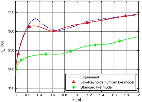
Figure 20: Comparison between inner wall temperature profile using Yang-Shih low-Reynolds number k-𝛆 model and Standard ―wall function‖ k-𝛆 model ... 23

Figure 21: Mesh adopted for the SWIRL code ... 27

Figure 22: Notation adopted for control volumes ... 28

Figure 23: Staggered mesh ... 28

Figure 24: Mesh adopted for FLUENT Code ... 32

Figure 25: Mesh adopted; STAR-CCM+ Code ... 36

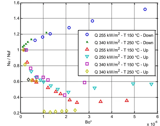
Figure 26: Watts experiments (Jackson, 2009a): Nusselt ratio versus Buoyancy parameter calculated by SWIRL using Yang-Shih turbulence model at x/L = 0.9 ... 41

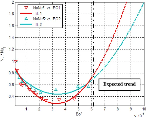
Figure 27: Watts experiment (Jackson, 2009a): Nusselt ratio versus Buoyancy parameter - trend lines ... 42

(12)

VIII

Figure 28: Watts experiments (Jackson, 2009a): Nusselt ratio versus Buoyancy parameter

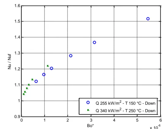
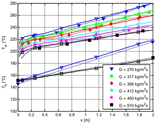
SWIRL code – YS turbulence model – downward flow ... 44 Figure 29: Comparison experimental (dotted line) and simulated (continuos line) inner wall and

bulk temperature; SWIRL code – YS turbulence model, Q = 255 W/m2, Tin = 150°C – downward flow ... 45 Figure 30: Nusselt ratio along the heated length; SWIRL code – YS turbulence model,

Q = 255 W/m2, Tin = 150°C – downward flow ... 45 Figure 31: Comparison experimental (dotted line) and simulated (continuos line) inner wall and

bulk temperature; SWIRL code – YS turbulence model, Q = 340 W/m2, Tin = 250°C – downward flow ... 46 Figure 32: Nusselt ratio along the axial line; SWIRL code – YS turbulence model,

Q = 340 W/m2, Tin = 250°C – downward flow ... 46 Figure 33: Radial velocity ratio profile; SWIRL code – YS turbulence model, Q = 255 W/m2,

Tin = 150°C - downward flow ... 47 Figure 34: Radial turbulent kinetic energy ratio profile; SWIRL code – YS turbulence model,

Q = 255 W/m2, Tin = 150°C – downward flow ... 47 Figure 35: Radial velocity ratio profile; SWIRL code – YS turbulence model, Q = 340 W/m2,

Tin = 250°C – downward flow ... 48 Figure 36: Radial turbulent kinetic energy ratio profile; SWIRL code – YS turbulence model,

Q = 340 W/m2, Tin = 250°C – downward flow ... 48 Figure 37: Watts experiments (Jackson, 2009a): Nusselt ratio versus Buoyancy parameter

SWIRL code – YS turbulence model – upward flow (selected cases) ... 49 Figure 38: Comparison of experimental (dotted line) and simulated (continuos line) inner wall

and bulk temperature; SWIRL code – YS turbulence model, Q = 255 W/m2,

Tin = 150°C – upward (1) ... 50 Figure 39: Comparison of experimental (dotted line) and simulated (continuos line) inner wall

Tin = 150°C – upward flow (2) ... 50 Figure 40: Comparison of experimental (dotted line) and simulated (continuos line) inner wall

Tin = 150°C – upward flow (3) ... 51 Figure 41: Nusselt ratio along the heated length; SWIRL code – YS turbulence model,

Q = 255 W/m2, Tin = 150°C – upward flow ... 51 Figure 42: Comparison experimental (dotted line) and simulated (continuos line) inner wall and

bulk temperature; SWIRL code – YS turbulence model, Q = 340 W/m2, Tin = 250°C – upward flow (1) ... 52 Figure 43: Comparison experimental (dotted line) and simulated (continuos line) inner wall and

bulk temperature; SWIRL code – YS turbulence model, Q = 340 W/m2, Tin = 250°C – upward flow (2) ... 52 Figure 44: Comparison experimental (dotted line) and simulated (continuos line) inner wall and

bulk temperature; SWIRL code – YS turbulence model, Q = 340 W/m2, Tin = 250°C – upward flow (3) ... 53 Figure 45: Nusselt ratio along the heated length; SWIRL code – YS turbulence model,

Q = 340 W/m2, Tin = 250°C – upward flow ... 53 Figure 46: Radial velocity ratio profile; SWIRL code – YS turbulence model, Q = 255 W/m2,

Tin = 150°C – upward flow (1) ... 54 Figure 47: Radial velocity ratio profile; SWIRL code – YS turbulence model, Q = 255 W/m2,

(13)

IX Figure 49: Radial turbulent kinetic energy ratio profile; SWIRL code – YS turbulence model,

Q = 255 W/m2, Tin = 150°C - upward flow (2) ... 55 Figure 50: Radial velocity ratio profile; SWIRL code – YS turbulence model, Q = 340 W/m2,

Tin = 250°C – upward flow (1) ... 56 Figure 51: Radial velocity ratio profile; SWIRL code – YS turbulence model, Q = 340 W/m2,

Tin = 250°C – upward flow (2) ... 56 Figure 52: Radial turbulent kinetic energy ratio profile; SWIRL code – YS turbulence model,

Q = 340 W/m2, Tin = 250°C - upward flow (1) ... 57 Figure 53: Radial turbulent kinetic energy ratio profile; SWIRL code – YS turbulence model,

Q = 340 W/m2, Tin = 250°C - upward flow (2) ... 57 Figure 54: Radial velocity ratio profile; SWIRL code – YS turbulence model – upward – cases

A: G~700 kg/sm2

... 59 Figure 55: Radial turbulent kinetic energy ratio profile SWIRL code – YS turbulence model –

upward flow - case A: G~700 kg/sm2

... 59 Figure 56: Radial velocity ratio profile; SWIRL code – YS turbulence model – upward flow-

case B: G~500 kg/sm2

upward flow - case B: G~500 kg/sm2

... 60 Figure 58: Radial velocity ratio profile; SWIRL code – YS turbulence model – upward flow –

case C: G~300 kg/sm2

upward flow - case C: G~300 kg/sm2

... 61 Figure 60: Comparison experimental (dotted line) and simulated (continuos line) inner wall;

SWIRL code – YS turbulence model, Q = 255 W/m2, Tin = 150°C, 200°C, 250°C, G = 284 kg/sm2 – upward flow ... 62 Figure 61: Radial velocity ratio profile and radial turbulent kinetic energy ratio profile; SWIRL

code – YS turbulence model, Q = 255 W/m2, Tin = 150°C, 200°C, 250°C,

G = 284 kg/sm2 – upward flow ... 62 Figure 62: Comparison between experimental and simulated inner wall temperature; SWIRL

code for different turbulence models, Q = 255 W/m2, Tin = 150°C – downward flow ... 63 Figure 63: Comparison between experimental and simulated inner wall temperature; SWIRL

code for different turbulence models, Q = 255 W/m2, Tin = 150°C – upward flow (1) .... 64 Figure 64: Comparison between experimental and simulated inner wall temperature; SWIRL

code for different turbulence models, Q = 255 W/m2, Tin = 150°C – upward flow (2) .... 64 Figure 65: Comparison between experimental and simulated inner wall temperature;

Q = 255 W/m2, Tin = 150°C – downward flow ... 65 Figure 66: Comparison between experimental and simulated inner wall temperature;

Q = 255 W/m2, Tin = 150°C – upward flow (1) ... 66 Figure 67: Comparison between experimental and simulated inner wall temperature;

Q = 255 W/m2, Tin = 150°C – upward flow (2) ... 66 Figure 68: Comparison between experimental and simulated inner wall temperature;

Q = 340 W/m2, Tin = 250°C, G = 392 kg/sm 2

– upward flow ... 67 Figure 69 Comparison between the inner wall temperature profiles obtained with different

meshes; STAR-CCM+ code, Lien turbulende model, Q = 340 W/m2, Tin = 250°C, G = 392 kg/sm2 – upward flow ... 68 Figure 70: Axial velocity and turbulent kinetic energy distributions (SWIRL code,YS

(14)

X

Figure 71: Nusselt ratio along the axial line; SWIRL code – YS turbulence model ... 71

Figure 72: Bulk velocity along the heated lenght ... 75

Figure 73: Bulk density along the heated length ... 76

Figure 74: Test section schematic for case 1 ... 78

Figure 75: Experimental data for case 1 ... 78

Figure 76: Test section schematic for case 2 ... 79

Figure 77: Comparison of experimental (dotted line) and simulated (continuos line) inner wall and bulk temperature; SWIRL code for different turbulence models, Q = 884 W/m2, Tin = 532°C, G = 1500 kg/sm 2_{– upward ... 80}

Figure 78: Comparison of experimental (dotted line) and simulated (continuos line) inner wall and bulk temperature; SWIRL code for different turbulence models, Q = 884 W/m2, Tin = 532°C, G = 1500 kg/sm2– upward ... 80

Figure 79: Velocity ratio profile and turbulent kinetic energy profile; SWIRL code for different turbulence models, Q = 884 W/m2, Tin = 532°C, G = 1500 kg/sm 2_{– upward ... 81}

Figure 81: Nusselt ratio along the heated length; SWIRL code for different turbulence models, Q = 400 W/m2, Tin = 250°C, G = 820 kg/sm 2_{– upward ... 82}

Figure 82: Velocity ratio profile and turbulent kinetic energy profile; SWIRL code for different turbulence models, Q = 400 W/m2, Tin = 250°C, G = 820 kg/sm 2_{– upward ... 83}

Figure 83: of experimental (dotted line) and simulated (continuos line) inner wall and bulk temperature; SWIRL code for different turbulence models, Q = 400 W/m2, Tin = 250°C, G = 892 kg/sm2– downward flow ... 84

Figure 84: Nusselt ratio along the heated length; SWIRL code for different turbulence models, Q = 400 W/m2, Tin = 250°C, G = 892 kg/sm 2_{– downward flow ... 84}

Figure 85: Velocity ratio profile and turbulent kinetic energy profile; SWIRL code for different turbulence models, Q = 400 W/m2, Tin = 250°C, G = 892 kg/sm 2_{– downward flow ... 85}

Figure 87: Nusselt ratio along the heated length; SWIRL code for different turbulence models, Q = 400 W/m2, Tin = 250°C, G = 380 kg/sm 2_{– upward ... 86}

Figure 88: Velocity ratio profile and turbulent kinetic energy profile; SWIRL code for different turbulence models, Q = 400 W/m2, Tin = 250°C, G = 380 kg/sm2– upward ... 87

Figure 89: Comparison of experimental (dotted line) and simulated (continuos line) inner wall and bulk temperature; SWIRL code for different turbulence models, Q = 400 W/m2, Tin = 250°C, G = 380 kg/sm 2_{– downward flow ... 88}

Figure 90: Nusselt ratio along the heated length; SWIRL code for different turbulence models, Q = 400 W/m2, Tin = 250°C, G = 380 kg/sm 2_{– downward flow ... 88}

Figure 91: Velocity ratio profile and turbulent kinetic energy profile; SWIRL code for different turbulence models, Q = 400 W/m2, Tin = 250°C, G = 380 kg/sm 2_{– downward flow ... 89}

(15)

XI

List of Tables

Table 1: Critical properties for common supercritical fluids ... ... 6

Table 2: Input conditions for upward flow ... ... 16

Table 3: Input conditions for downward flow ... ... 16

Table 4: Constants in the turbulence models ... ... 22

Table 5: Functions appearing in the turbulence models ... ... 22

Table 6: D, E and T terms ... ... 22

Table 7: Typical mesh detail (axial and radial) for SWIRL... ... 27

Table 8: Typical mesh detail (axial x radial) for FLUENT... ... 32

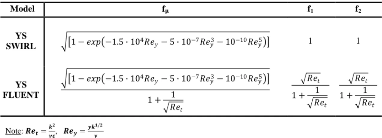
Table 9: SWIRL and FLUENT damping functions for the Yang-Shih turbulence model... ... 34

Table 10: Typical mesh detail (axial x radial); STAR-CCM+ ... ... 35

Table 11: Watts experiments (Jackson, 2009a): simulated ... ... 40

Table 12: Watts experiments (Jackson, 2009a): selected simulated cases ... ... 43

Table 13: Watts experiments (Jackson, 2009a): downward flow cases simulated ... ... 44

Table 14: Watts experiments (Jackson, 2009a): upward flow cases simulated ... ... 49

Table 15: Watts experiments (Jackson, 2009a): upward flow cases simulated at a same mass flux ... . ... 58

Table 16: Watts experiments (Jackson, 2009a): upward flow case simulated to compare different turbulence models ... ... ... 63

Table 17: Geometry and test parameters; Case 1 ... ... 78

(16)

(17)

XIII

List of Symbols

Roman Letters Bo* Buoyancy parameter D Pipe inner diameter [m] fA,R,λ Model functions fw Wall distance function fμ Damping function

g Gravitational acceleration 𝑚

𝑠2 G Mass flux _𝑠∙𝑚𝑘𝑔₂

Gk Gravitational production term Gr Grashof number

h Enthalpy _𝑘𝑔𝐽

k Turbulent Kinetic Energy 𝑚2

𝑠2 Nu Nusselt number Nu Nuf Nusselt ratio Pr Prandtl number Q Heat flux _𝑚𝑊₂ r Radial coordinate [m] R Time scale ratio Re Reynolds number

Sij second-moment closure term Sk Shear production term T Temperature [°C]

ut Friction velocity scale uε Kolmogorov velocity scale U, u Velocity component in the

x-direction

V, v Velocity component in the r-direction

x Axial coordinate [m] y+, Ry a-dimensional distance

Greek Letters α Heat transfer coefficient αt Eddy diffusivity β Thermal expansion _𝐾1 δij Kronecker delta ε Dissipation Rate of k 𝑚_𝑠₃2 λ Thermal conductivity _𝑚∙𝐾𝑊 μ (Molecular) viscosity _𝑠∙𝑚𝑘𝑔 ρ Density _𝑚𝑘𝑔₃ σT Turbulent Prandtl τk Kolmogorov time scale τt Characteristic time scale τij Reynolds stress tensor

(18)

XIV Subscript 0 Ideal b Bulk cr Critical e Effective f Forced pc Pseudocritical T Turbulent w Wall n, s,

e, w North, South, East, West grid point N, S,

E, W North, South, East, West surface

Abbreviations BWR Boiling Water Reactor

CFD Computational Fluid Dynamics IAEA

-CRP International Atomic Energy Agency – Coordinated Research Project RANS Reynolds-Averaged Navier-Stokes

(19)

1

Introduction

General Background

The largest industrial application of supercritical fluids in the energy sector is currently related to fossil-fired power plants where, in particular, water at supercritical pressure is used. The idea to use supercritical water steam to increase the thermal efficiency of fossil-fired power plants received increasing attention in the period from the 1950s-1980s in USA and USSR.

However, the first contributions to the study of the problems related to heat transfer with fluids at supercritical pressure started in 1930s with the investigation on free convection in fluids near the pseudo-critical temperature. The objective was to develop a new effective cooling system for turbine blades in jet engines (Schmidt, et al., 1946; Schmidt, 1960). Already in these studies, the advantages offered by single-phase thermosyphons with the intermediate working fluid at pseudocritical temperature were pointed out.

It is well known that, at supercritical pressures, fluids show thermal-hydraulic characteristics quite different from those of conventional sub-critical pressure conditions. In particular, the physical properties of fluids at supercritical pressure change significantly near the pseudocritical temperature, without any liquid-vapor phase transition; this feature, occurring in a narrow range of operating parameters, completely alters the turbulent flow structure, possibly causing even heat transfer deterioration.

In 2000s, the idea to use supercritical steam water combined with the Best Available Technologies (BAT) for fossil power plants received further attention (European Commission, Bref, 2006): for example the Circulating Fluidized Bed Combustion (CFBC) has established its position as utility scale boiler technology and it is ready to be operated with supercritical steam parameters and larger boiler sizes. In March of 2009, the 460 MWe supercritical CFBC boiler of Łagisza (Poland) has reached operation at full load. It was built by the Polish utility company Poludniowy Koncern Energetyczny SA together with the American energy utility Foster Wheeler Energia Oy Group. The Łagisza power plant is the first supercritical once-through CFBC boiler (BENSON) in the world with the operating temperature of 560 °C and operative pressure of 27,5 MPa (Venalainen, 2003).

Concerning the field of nuclear energy, in the ’60s some studies were carried out to investigate the possibility to use supercritical water as coolant in nuclear reactors. One of the advantages of this

(20)

2

proposal was the low coolant mass-flow rates needed for cooling the core due to the considerable increase of specific enthalpy at supercritical conditions. Using supercritical water, the efficiency of the modern nuclear plant could rise from the current figure of 33–35%, to ~40% or more, leading also to benefits in terms of decrease of the operational and capital costs by eliminating steam generators, steam separators, steam dryers, etc.

The Supercritical Water-cooled Reactor (SCWR) is one of the six candidates selected by U.S. DOE and Generation IV International Forum for the next generation of nuclear reactors (U.S. Department of Energy Office of Nuclear Energy, 2003). Obviously, the supercritical pressure water-cooled nuclear reactors can compete in terms of cost, safety and reliability with other types of power generation systems, even if the SCWR requires significant development of materials and structures due to the corrosive high-temperature supercritical water environment.

Additional applications of supercritical pressure fluids are the oxidation systems for waste processing (Zhou, et al., 2000), the use of carbon dioxide at supercritical pressure in a new generation of air-conditioning systems for cars and refrigeration systems (Pitla, et al., 1998) and the liquid hydrogen-oxygen fuelled rockets (Youn, et al., 1993). Frequently, supercritical fluids are used also to replace Freons and certain organic solvents in some industrial application.

Motivation for the present work

Computational fluid dynamics (CFD) uses numerical methods and algorithms to solve and analyze problems which involve fluid flows. In these years, major efforts are devoted to improving the performance and the speed of CFD models when applied to complex flow simulations; in this process, the need is felt for validating CFD codes and their performances on new applications to understand the accuracy offered in representing the addressed phenomena.

In particular, regarding supercritical fluids, most existing codes, including those used in present work, need to be extended with respect to their initial purpose and improved to model the peculiar phenomena observed in the behaviour of these fluids. So, appropriate predictive models for computing heat transfer to supercritical fluids need to be incorporated into the CFD codes and then need to be tested and validated.

The aim of the present work is to validate the capabilities of different codes and different turbulence models in predicting heat transfer enhancement or deterioration and wall temperature trends for particular operating conditions, using fluid at supercritical pressure in downward and upward flow through circular pipes. Because of the enhancement and deterioration of heat transfer, for supercritical flows it is necessary to have precise information in establishing the thermal limits reached within the system. Moreover, the difficulties in performing calculations are several due to the non-uniformity of thermal properties and the related numerical phenomena that this feature involve.

The validation of CFD codes is aimed at defining the extent at which they are capable to handle the relevant phenomena observed in flow systems. In particular, for nuclear applications, the design of a SCWR core requires a reliable database on the thermal hydraulic characteristics of supercritical water flows in proposed geometries and operation conditions. A lot of data has been accumulated for large tubes in the field of fossil-fired power plants operating at supercritical pressure; however, in the literature, the data for a narrow geometry, which is typical for the SCWR power plant, are limited and sometimes there are considerable differences in published data. The collection and evaluation of existing data, as well as conducting new experiments for specified geometry, is

(21)

3 necessary to establish accurate methods and techniques for the prediction of heat transfer in SCWR cores.

In support of efforts of member states in the area of SCWRs, the International Atomic Energy Agency (IAEA) started in 2008 the Coordinated Research Programme (CRP) on "Heat Transfer

Behaviour and Thermo-hydraulics Codes Testing for SCWRs" (IAEA, 2009). This IAEA CRP

promotes an international collaboration among IAEA Member States for the development of Supercritical Water-Cooled Reactors in the areas of thermo-hydraulics and heat transfer, including the collection of experimental data relevant to supercritical fluid behaviour as well as the development and testing of the associated computer methods. The two key objectives of this CRP are:

1- to establish a base of accurate data for heat transfer, pressure drop, blowdown, natural circulation and stability for conditions relevant to supercritical fluids;

2- to test methods for the analysis of SCWR thermo-hydraulic behaviour, identifying the code development needed.

The University of Pisa and the University of Manchester are two of the twelve institutions that participate in this CRP. The present work was developed during a four months period at the University of Pisa and three months period at the University of Aberdeen, in order to develop the work under the direct guidance of the foreign tutors of this thesis and to make use of a code, SWIRL, available at that Institution. The Universities of Pisa, Manchester and Aberdeen are involved in a trilateral co-operation programme which provided support for the student exchange programme.

Thesis outline

This work is subdivided into five chapters: after a general introduction on supercritical fluids and their thermal and fluid-dynamic characteristics (Chapter ‎1), a detailed description of the considered experimental facility (Jackson, 2009a) is proposed (Chapter ‎2). A description of the CFD codes adopted in the work (SWIRL, a ―in-house‖ CFD code (He, et al., 2003); FLUENT and STAR-CCM+, general-purpose CFD codes (FLUENT, 2005; Cd-adapco, 2009)) is then proposed, with attention to the adopted turbulence models (AKN (Abe, et al., 1994a), LS (Launder, et al., 1974), YS (Yang, et al., 1993) and Lien (Lien, et al., 1996)) (Chapter ‎3); the rationale at the basis of the different low-Reynolds number models and the different features introduced to extend their use are given particular attention.

A detailed analysis of the achieved results is proposed (Chapter ‎4), comparing the experimental value of wall temperature with that predicted by the different turbulence models selected and the different CFD codes used. Radial profiles of the dimensionless velocity (velocity over bulk velocity) and of the dimensionless turbulent kinetic energy (turbulent kinetic energy over the square of bulk velocity) are analyzed, for different axial locations along the pipe and for a selected number of significant cases in both downward and upward flow. Meanwhile, it is also proposed an analysis of the heat transfer behaviour trying to explaining the differences between the deterioration and the enhancement phenomena and between the buoyancy and the acceleration effects that characterize this kind of application. Finally, a summary of the main attained conclusions is provided and recommendations for future works are proposed.

In the appendices, some values of significant parameters useful for the data analysis (Appendix A) and the data obtained in additional simulations performed for the computational benchmark exercise ―Pipe with heating‖ proposed by the IAEA CRP (Appendix B) are reported.

(22)

(23)

5

Chapter 1.

1. Features of supercritical fluids

In this Chapter the main features of supercritical fluids are presented: physical, thermal and dynamic aspects are analysed and considerations on heat transfer are carried out.

1.1. Thermodynamic characteristics

The supercritical region of a pure fluid is shown in Figure 1 and, as defined in literature (Kirk, et al., 2007), it represents the area bounded by the critical pressure and critical temperature.

Figure 1: Schematic P-T diagram

The particular feature of supercritical fluids is that they change in a continuous manner from being liquid-like to gas-like as the temperature is increased over a specific value (pseudo-critical temperature Tpc). This unique attribute of supercritical fluids may be shown by the Figure 1:

the P-T diagram can be analyzed beginning from point A in the subcritical liquid zone. If the liquid is depressurized isothermally from point A to point E, the vapor pressure line is crossed meanwhile if the liquid takes the path line A–B–C–D–E, the fluid passes from a liquid phase to a gas phase and no meniscus is seen. Common applications of supercritical fluids operate near point C, where the density and diffusivity of the fluid is relatively high while the viscosity remains low. However, when heat takes place in this condition, extreme non-uniformities of physical and transport properties can be present.

Supercritical fluid region

(24)

6

Frequently the term compressed fluid is used instead of supercritical fluid. A compressed fluid is a more general expression to indicate fluid than can be a supercritical fluid, a near-critical fluid, an expanded liquid, or a highly compressed gas, depending on temperature, pressure, and composition.

Carbon dioxide is of particular interest. It has relatively low critical temperature (31 °C) and pressure (7.38 MPa); it is non-flammable, essentially non-toxic, and environmentally friendly especially when is used to replace Freons and certain organic solvents. Moreover, CO2 is the second least expensive solvent after water.

Water has an unusually high critical temperature (374 °C) owing to its polarity. Water at supercritical conditions can dissolve gases, e.g., O2 and no polar organic compounds. This phenomenon is interesting for oxidation of toxic wastewater and hydrothermal synthesis.

Many of the other supercritical fluids commonly available are listed in Table 1 with respective critical temperature, pressure and density; however, the ultimate choice for a specific application is depending on additional factors, e.g., safety, flammability, phase behaviour, solubility, and cost.

Table 1: Critical properties for common supercritical fluids (Kirk, et al., 2007)

SOLVENT Tcr [°C] Pcr [MPa] 𝛒cr [g/cm3] SOLVENT Tcr [°C] Pcr [MPa] 𝛒cr [g/cm3] Ethylene 9.3 5.04 0.22 Ammonia 132.5 11.28 0.24 Xenon 16.6 5.84 0.12 N-nutane 152.1 3.80 0.23

Carbon dioxide 31.1 7.38 0.47 N-pentane 196.5 3.37 0.24

Ethane 32.2 4.88 0.20 Isopropanol 235.2 4.76 0.27

Nitrous oxide 36.5 7.17 0.45 Methanol 239.5 8.10 0.27

Propane 96.7 4.25 0.22 Toluene 318.6 4.11 0.29

Water 374.2 22.05 0.32

In the following figures the main physical and thermodynamic characteristics of these fluids are shown as functions of temperature and pressure, in particular for water (data are taken from Sharabi, 2008). In a narrow temperature range, the density decreases sharply, in particular close to the critical pressure as it can be seen in Figure 2; so, the fluid changes gradually and without discontinuities from a high density-like liquid to a low density-like gas.

Figure 2: Water density trends (Sharabi, 2008)

Specific Heat has a different behaviour because the transition from liquid-like to gas-like fluid

is accompanied by a sharp peak, as it is shown in Figure 3. The temperature at which the specific heat reaches a maximum is called ―pseudo-critical temperature‖ and is identified by Tpc; the maximum specific heat decreases with increasing pressure (see Figure 4). Moreover, it is possible to note that the

(25)

7 locus of temperatures at which the specific heat at constant pressure reaches a maximum, (pseudo-critical line), is the extension of the saturation line in the super(pseudo-critical region (see Figure 5).

Figure 3: Water specific heat trends as a function of Temperature (Sharabi, 2008)

Figure 4: Water specific heat as a function of Pressure (Sharabi, 2008)

Figure 5: Water saturation a Pseudo-critical line (Sharabi, 2008)

Due to the previous considerations on specific heat, the enthlapy of supercritical fluids sharply increases with temperature close to the pseudo-critical temperature, as shown in Figure 6.

Figure 6: Water enthalpy trends (Sharabi, 2008)

In Figure 7 and Figure 8 the trends of thermal conductivity and of molecular viscosity are shown; they are quite similar except for the peak of thermal conductivity near the pseudocritical temperature, occurring when pressure is close to the critical one.

(26)

8

Figure 7: Water thermal conductivity trends

(Sharabi, 2008) Figure 8: Water molecular viscosity trends

(Sharabi, 2008)

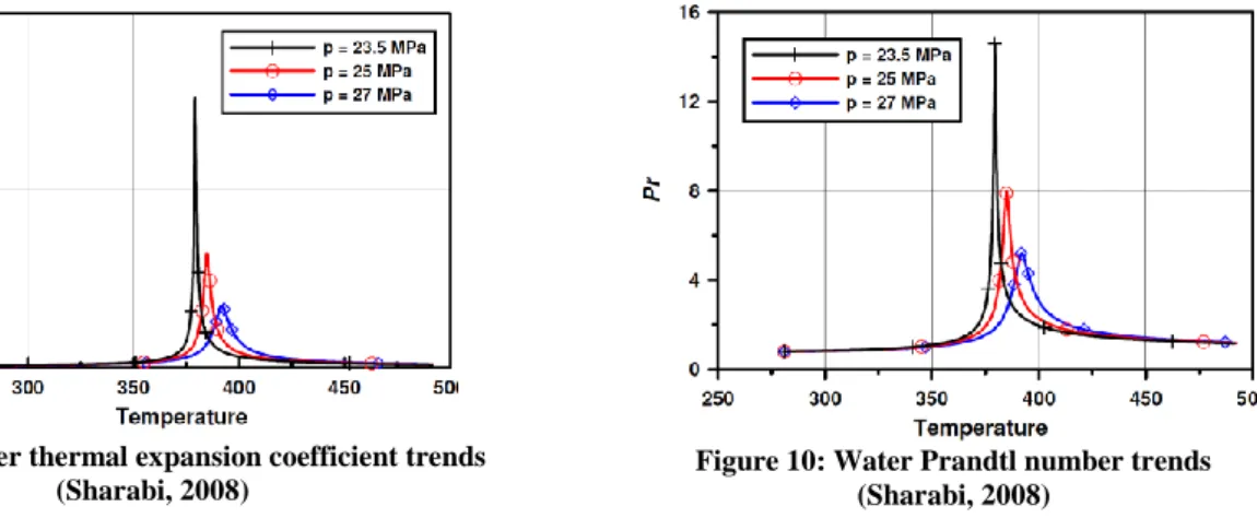
In similarity with the trend of the specific heat, the thermal expansion coefficient and the

Prandtl number have also a pronounced peak near the critical conditions (Figure 9 and Figure 10).

Figure 9: Water thermal expansion coefficient trends (Sharabi, 2008)

Figure 10: Water Prandtl number trends (Sharabi, 2008)

It is also interesting to analyze these properties depending on enthalpy as shown in Figure 11. Unlike the profiles dependent on temperature, in this case it is possible to note a smoother change of the trends across the critical conditions, due to the large internal energy gained by the fluid during the heating at these conditions.

(27)

9

1.2. Heat transfer characteristics

Heat transfer with fluids near the critical conditions is more complex than for ordinary fluids. In heat transfer applications involving supercritical fluids, the diffusion of heat can be strongly influenced by the variations of properties mentioned in Paragraph ‎1.1. In particular, the variation of density can affect turbulent production. This phenomenon is due to the influence of buoyancy or to the flow acceleration, both caused by heating. This can cause very significant localised distortions of the mean flow and turbulent fields, resulting in effects such as laminarization. In this case, it is important to decide the type of heat transfer occurring in the particular conditions, i.e., forced convection or mixed convection: under forced convection, buoyancy is considered insignificant, meanwhile under mixed convection the density changes are more significant.

To show this particular aspect, the results and conclusions of some studies published in literature reported and summarized (He et al., 2007; Song, et al., 2007; He et al., 2008; Sharabi, 2008; Jackson, 2009b).

1.2.1. Forced convection

In this kind of application, the velocity profile has the standard shape, flattened soon after the beginning of the heating under the influences of flow acceleration. This is due to expansion of fluid with increasing temperature. Thus, this mechanism does not show significant application problems related to the heat transfer and is simple to be simulated by CFD codes.

1.2.2. Mixed convection

1.2.2.1. Influence of buoyancy

In mixed convection, the effectiveness of heat transfer is affected by buoyancy. As discussed by He et al. (2007), buoyancy can modify turbulence by two different mechanisms, causing the enhancement or suppression of the turbulence production. So, it is possible to distinguish the direct (structural) effect, through buoyancy-induced production of turbulent kinetic energy, and the indirect (external) effect, through the modification of the mean flow. For mixed convection in a vertical channel, the indirect effect is normally the dominant one.

For downward flow (buoyancy-opposed flows in a heated passage), the influence of buoyancy causes the reduction of velocity near the wall, while it is possible to note an increase of it in other region of the tube. This modification of the mean flow field causes an enhancement of turbulence production and improves turbulent diffusion and heat transfer in general.

For upward flow (buoyancy-aided flows in a heated passage), the influence of buoyancy causes a flattened velocity gradient of flow with the exception of zone near the wall. So, in this way the turbulence production is reduced and the heat transfer is weakened. For these reasons it is easy to note that if buoyancy is progressively increased, by reducing the flow rate and/or increasing the heating rate, the impairment of turbulence production and the deterioration of heat transfer become more and more marked. Still in literature (McEligot, et al., 2004; He, et al., 2007; Sharabi, et al., 2009), it is usual to refer at this case with the expression laminarization of the flow: flows considered to be turbulent show heat transfer parameters as low as in laminar flows; in this way, with further increase of buoyancy influence, negative values of shear stress are generated in the core region. Thus,

(28)

10

turbulence can be produced directly there and the heat transfer improved. This happens immediately and it is followed by further distortions giving rise to an inverted M-shaped profile.

Moreover, in literature it is possible to find criteria for the occurrence of the laminarization phenomenon (Jackson, et al., 1979; McEligot, et al., 2004; Jackson, 2009b). In particular, a simple criterion to consider negligible the effect of buoyancy is provided by equation ‎(1.1).

𝑮𝒓_𝒃∗

𝑹𝒆_𝒃𝟑.𝟓_𝑷𝒓𝟎.𝟖< 3 ∙ 𝟏𝟎−𝟕 (1.1)

On the other hand, a criterion to consider negligible the effect of flow acceleration is provided by equation ‎(1.2). 𝑸_𝒃∗ 𝑹𝒆_𝒃𝟏.𝟔𝟐𝟓_𝑷𝒓 𝒃 < 2 ∙ 𝟏𝟎−𝟔 (1.2)

1.2.2.2. Influence of flow acceleration

Turbulent heat transfer in channels can also be significantly affected by flow acceleration caused by thermal expansion of the fluid due to strong heating as previously noted in Figure 9. As a fluid flows along a heated pipe, its bulk temperature and enthalpy increases while density falls; the mass flow is the same at all axial positions; so, the bulk velocity increases.

In this way, the velocity profile is modified determining the inhibition of turbulent production and turbulent diffusion.

(29)

11

1.2.3. Heat transfer deterioration

The deterioration phenomenon occurs when the pseudocritical temperature is reached.

In literature there are different methods to evaluate the deterioration: for example, it is possible to define the Deterioration ratio _𝛼𝛼

0 (see Figure 12), where α0 is the ―ideal‖ heat transfer coefficient (Koshizuka et al., 1995). The onset of deterioration is evaluated when this ratio is smaller than 0.3.

Figure 12: Heat transfer deterioration at various flow rates (Koshizuka, et al., 1995)

It is possible to note that the heat transfer coefficient monotonically decreases with increasing heat flux when the flow rate is large, while it abruptly collapses maintaining a constant value when the flow rate is small.

(30)

12

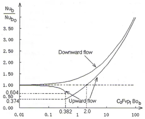
In literature (McEligot, et al., 2004; He, et al., 2008; Jackson, 2008; Jackson, 2009c) is also proposed to define the Nusselt ratio _𝑁𝑢𝑁𝑢

𝑓 as another equivalent method to evaluate deterioration, where Nu is Nusselt number in mixed convection and Nuf is Nusselt number in forced convection.

Analyzing the variation of the ratio with a parameter that takes in account the buoyancy effect is possible to understand the deterioration of heat transfer and also the enhancement phenomenon, as it possible to see in Figure 13. For this reason, this approach was used in the present work to analyze the heat transfer behaviour.

Figure 13: Overall picture of buoyancy-influenced heat transfer for upward and downward flow (Jackson, 2009c)

A Nusselt ratio greater than unity means that heat transfer is more effective than in forced convection and viceversa when the ratio is lower than unity. In Figure 13, it is possible to recognize that the heat transfer behaviour can change with the increasing of the effect of buoyancy. This can be done acting on the value of mass flux.

The above considerations about Figure 12 and Figure 13 suggest that there are various mechanisms of deterioration as function of flow rate.

(31)

13

1.2.3.1. Heat transfer deterioration at low flow rate

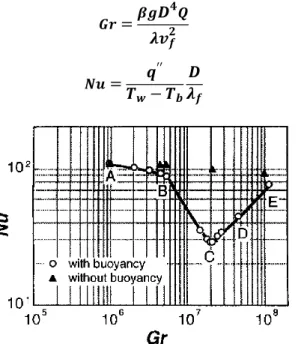
To understand this mechanism, it is possible to refer to Figure 14, where the relation between the Nusselt number and the Grashof number (related to the ratio of buoyancy to viscous forces) is shown.

𝑮𝒓=𝜷𝒈𝑫 𝟒_𝑸 𝝀𝒗𝒇𝟐 (1.3) 𝑵𝒖=_𝑻 𝒒′′ 𝒘− 𝑻𝒃 𝑫 𝝀𝒇 (1.4)

Figure 14: Relationship between Nusselt number and Grashof number (Koshizuka, et al., 1995) Flow rate G = 39 _𝒎𝑲𝒈𝟐_𝒔; Heat flux

𝑾

𝒎𝟐 : A = 100, B = 450, C = 550, D = 2000, E = 10000.

In Figure 14 it is noted that in the case with buoyancy, the Nusselt number keeps constant when the Grashof number is relatively low (forced convection); then, it shows a minimum value at Gr = 2 ∙ 107 and finally it increases again for larger Grashof number values (natural convection). The minimum point is suggested as the boundary between the two convection modes.

When the heat flux is large, the flow velocity increases near the wall and the profile becomes flattened, so that turbulence is reduced and heat transfer is deteriorated. Moreover, when the heat flux is even more increased after the minimum heat transfer point, the flow velocity profile is increasingly deformed and turbulent heat transfer is improved (see Figure 15 and Figure 16).

Figure 15: Radial distribution of flow velocity G = 39 _𝒎𝑲𝒈_𝟐_𝒔, Heat flux _𝒎𝑾_𝟐 : A = 100; B = 450; C = 550;

D = 2000; E = 10000 (Koshizuka, et al., 1995)

Figure 16: Radial distribution of turbulence energy G = 39 _𝒎𝑲𝒈_𝟐_𝒔, Heat flux _𝒎𝑾_𝟐 : A = 100; B = 450; C = 550;

(32)

14

1.2.3.2. Heat transfer deterioration at high flow rate

As shown in Figure 17, when the heat flux increases, the turbulence kinetic energy decreases near the wall. The kinematic viscosity increases and the Prandtl number decreases locally since the temperature is increased because of heating. A larger kinematic viscosity leads to a thicker viscous sub-layer, which reduces turbulence near the wall and heat transfer is deteriorated. Moreover, especially at high flow rates, the increasing of temperature determines the density decrease and the Prandtl number decreases with the density: smaller Prandtl number reduces the heat transfer amplyfing the effect due to large viscosity. At small Prandtl number, deterioration occurs only in upward flow and not in downward flow because the buoyancy and laminarization mainly govern the amount of deterioration. In this case, a sharp increase of wall temperature takes place: when heat flux is imposed, if the temperature at the wall is close to the pseudocritical value, the consequent change of fluid proprieties in the boundary layer determines the deterioration, since the resulting wall temperature increase tends to worsen deterioration.

Figure 17: Radial distributions near the wall (Koshizuka, et al., 1995)

(33)

15

Chapter 2.

2. Considered experiments

In this Chapter the natural circulation test facility used by M. J. Watts in his PhD study in 1970s is described. The study addressed both forced and mixed convection heat transfer using a vertical tube test section with upward and downward flow (Jackson, 2009a). These results are used to validate the computational models.

2.1. Natural circulation test facility

Hereafter, the most important features of the supercritical pressure water flow loop adopted by Watts in his PhD study (Jackson, 2009a), showed in Figure 18, are presented.

2.1.1. Basic design parameters

The basic design parameters adopted for the supercritical pressure water flow loop, used to achieve the experiments, were reported as follows (Jackson, 2009a):

- Design pressure: 310 bar.

This allowed performing tests at the critical pressure of 221.2 bar and beyond;

- Design temperature: 450 °C.

This allowed performing tests where fluid bulk temperatures can be either below or above the critical temperature of 374.15 °C;

- Test section sizes: a pipe with a diameter of 25.4 mm (1‖) and a heated length of 2 m.

The test section diameters were chosen to be similar to those in steam generators for supercritical pressure thermal power plants in the case of forced circulation boilers. The pipe length was limited by the height of the laboratory;

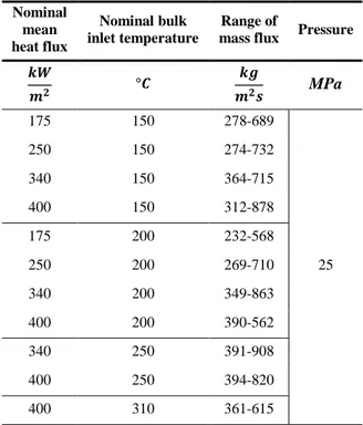
- Heat flux and mass velocity: many tests were performed, whose values of heat and mass flux are as shown in Table 2 and Table 3.

(34)

16

2.1.2. Test facility

Considering the selected design parameters, the closed arrangement layout and the natural circulation were adopted (Jackson, 2009a). In the nuclear engineering laboratory at the University of Manchester, as depicted in Figure 18, coolers could be located on the roof and the experimental area in the basement, with a vertical distance of 23 m between them. As said before, the vertical available test section was limited at 2 m by the height of the laboratory.

The test section was heated with ohmic heating, by alternating current supplied with two rectangular plates welded to the tube, as shown in Figure 19. Six transformers of 16 kVA were used, connected either in parallel or in series to obtain the most flexible arrangement. The cooler was located at the roof level and was capable to rejecting the equal amount of heat supplied by transformers. It used air cooling on the outside of the tube; so, the limiting heat transfer coefficient was related to air velocity.

The design approach for achieving downward flow in the test section required some care; in fact, for downward circulation it was possible to obtain a stable condition that once started should continue, using an auxiliary heater placed in the zone where the fluid has to rise. Once the correct circulation is achieved, it is possible to switch off the auxiliary heater and to gradually increase the ohmic heating until the desired value.

For each test performed, the test section outer wall temperature, the test section inlet and outlet water temperature, the test section inlet and outlet pressure and the test section inlet and outlet mass flow rate are accounted. The inner wall temperature profiles are derived from outer wall temperature values.

Table 2: Input conditions for upward flow Nominal mean heat flux Nominal bulk inlet temperature Range of

mass flux Pressure

𝒌𝑾 𝒎𝟐 °𝑪 𝒌𝒈 𝒎𝟐_𝒔 MPa 175 150 278-689 25 250 150 274-732 340 150 364-715 400 150 312-878 175 200 232-568 250 200 269-710 340 200 349-863 400 200 390-562 340 250 391-908 400 250 394-820 400 310 361-615

Table 3: Input conditions for downward flow Nominal mean heat flux Nominal bulk inlet temperature Range of

mass flux Pressure

𝒌𝑾 𝒎𝟐 °𝑪 𝒌𝒈 𝒎𝟐_𝒔 MPa 175 150 193-617 25 250 150 270-510 340 150 347-901 400 150 279-936 170 200 282-712 250 200 208-785 340 200 376-925 400 200 374-957 340 250 391-958 400 250 367-1011 400 290/310 330-966 400 310/320 569-834 430 280 215-624 450 300 375-1062 435 318 412-982

(35)

17

(36)

18

(37)

19

Chapter 3.

3. Numerical modelling approach

This Chapter reports the mathematical formulations of the general differential equations that govern transport and heat transfer phenomena involving fluid flow in turbulent conditions.

A brief description of the codes adopted in the study (SWIRL, an “in-house” CFD code, and FLUENT and STAR-CCM+, general-purpose CFD codes) is also reported.

3.1. Reynolds-Averaged Navier-Stokes Equations

The phenomena investigated in this work are analysed by the Reynolds-Averaged Navier-Stokes (RANS) Equations, along with the equations of energy conservation and continuity constituting a set of non-linear coupled, elliptic partial differential equations. To simulate turbulence transport other partial difference equations with different formulations and closure models are considered, with the aim to investigate the performance of different codes and turbulence models.

3.1.1. Governing equations

The governing equations are the steady turbulent flow equations of continuity, momentum and energy in a cylindrical coordinate system using the finite volume scheme (Patankar, 1980; Versteeg, et al., 1995). - Continuity equation 𝝏 𝝏𝒙 𝝆𝑼 + 𝟏 𝒓 𝝏 𝝏𝒓 𝝆𝒓𝑽 = 𝟎 (3.1)

It is possible to note that fluid density is under the sign of derivation to take into account its variation with pressure and temperature as seen in Chapter ‎1.

(38)

20 - U-momentum equation 𝝏 𝝏𝒙 𝝆𝑼𝟐 + 𝟏 𝒓 𝝏 𝝏𝒓 𝝆𝒓𝑼𝑽 = −𝝏𝒑 𝝏𝒙+ 𝝆𝒈𝒙 + 𝟐 𝝏 𝝏𝒙 𝝁𝒆 𝝏𝑼 𝝏𝒙 + 𝟏 𝒓 𝝏 𝝏𝒓 𝒓𝝁𝒆 𝝏𝑼 𝝏𝒓+ 𝝏𝑽 𝝏𝒙 (3.2) - V-momentum equation 𝝏 𝝏𝒙 𝝆𝑼𝑽 + 𝟏 𝒓 𝝏 𝝏𝒓 𝝆𝒓𝑽𝟐 = −𝝏𝒑 𝝏𝒓+ 𝝏 𝝏𝒙 𝝁𝒆 𝝏𝑽 𝝏𝒙+ 𝝏𝑼 𝝏𝒓 + 𝟐 𝒓 𝝏 𝝏𝒓 𝒓𝝁𝒆 𝝏𝑽 𝝏𝒓 − 𝟐 𝝁𝒆𝑽 𝒓𝟐 (3.3)

It is possible to note that the Reynolds stresses, resulting from the process of averaging the instantaneous Navier-Stokes equations, are assumed to be proportional to the mean rates of deformation by the turbulent viscosity μT, as suggested by the Boussinesq approximation. The

effective viscosity μe used in momentum equation, defined by μe = μ + μT (respectively molecular and

turbulent viscosity), implies that the viscous stresses are always considered, also when their effect is not negligible if compared with Reynolds stress.

- Energy equation (enthalpy based)

𝝏 𝝏𝒙 𝝆𝑼𝑯 + 𝟏 𝒓 𝝏 𝝏𝒓 𝝆𝒓𝑽𝑯 = 𝝏 𝝏𝒙 𝝁 𝑷𝒓+ 𝝁𝑻 𝝈𝑻 𝝏𝑯 𝝏𝒙 + 𝟏 𝒓 𝝏 𝝏𝒓 𝒓 𝝁 𝑷𝒓+ 𝝁𝑻 𝝈𝑻 𝝏𝑯 𝝏𝒓 (3.4)

- Energy equation (temperature based)

𝝏 𝝏𝒙 𝝆𝑪𝒑𝑼𝑻 + 𝟏 𝒓 𝝏 𝝏𝒓 𝝆𝑪𝒑𝒓𝑽𝑻 = 𝝏 𝝏𝒙 𝑪𝒑 𝝁 𝑷𝒓+ 𝝁_𝑻 𝝈𝑻 𝝏𝑻 𝝏𝒙 + 𝟏 𝒓 𝝏 𝝏𝒓 𝒓𝑪𝒑 𝝁 𝑷𝒓+ 𝝁_𝑻 𝝈𝑻 𝝏𝑻 𝝏𝒓 (3.5)

In both expressions of energy equations, σT is the turbulent Prandtl number, assigned to a

value of 0.9, as suggested by common practice with usual fluids.

It is possible to note that the energy equation can be written with two different formulations, in terms of enthalpy or expressed by temperature. Both are derived by the enthalpy transport equation (Kim, et al., 2010). Using the enthalpy formulation or the temperature formulation depends on the particular addressed problem: for example when problems with material interfaces are discretized, such as a solid-fluid interface that determines a discontinuities of enthalpy, but the temperature is continuous, the temperature formulation is very attractive because the temperature is directly obtained from the equation and heat transfer problems are simply solved.

Regarding the supercritical fluid could be better to use the enthalpy formulation because of the stronger variation of fluid properties with temperature near the pseudo-critical temperature, while the variation with enthalpy is smoother (see Figure 11). The temperature based expression can create severe numerical instabilities leading to convergence difficulties.

(39)

21

3.2. Adopted turbulence models

To simulate the flow field using Reynolds-Averaged two-equation models, two different transport equations are generally used to evaluate the local value of the turbulent kinetic energy and the integral turbulent length scale. In this work, the k-𝜀 turbulence model is used, where k is the turbulent kinetic energy and 𝜀 is its dissipation rate.

The standard k-𝜀 turbulence model uses ―wall functions‖ to simulate the viscous near-wall region, where the standard model is not valid due to the assumptions adopted in its derivation.

To better predict the phenomena occurring in this region, as an alternative it is possible to introduce low-Reynolds turbulence models that use viscous corrections to allow for integration through the viscous sub-layer.

In this work some low-Reynolds number eddy viscosity turbulence models are used. In particular those proposed by Abe, Kondoh and Nagano (AKN, Abe, et al., 1994), Launder and Sharma (LS, Launder, et al., 1974), Yang and Shih (YS, Yang, et al., 1993) and Lien, Chen and Leschziner (LIEN, Lien, et al., 1996). These models are commonly implemented in all general-purpose CFD codes.

The general equations for turbulence quantities in these models are:

- Turbulent Kinetic Energy (k)

𝝏 𝝏𝒙 𝝆𝑼𝒌 + 𝟏 𝒓 𝝏 𝝏𝒓 𝝆𝒓𝑽𝒌 = 𝝏 𝝏𝒙 𝝁 + 𝝁_𝑻 𝝈_𝒌 𝝏𝒌 𝝏𝒙 + 𝟏 𝒓 𝝏 𝝏𝒓 𝒓 𝝁 + 𝝁_𝑻 𝝈_𝒌 𝝏𝒌 𝝏𝒓 + 𝑷_𝒌+ 𝑮_𝒌− 𝝆𝜺 − 𝝆𝑫 (3.6) - Dissipation Rate (𝜀) 𝝏 𝝏𝒙 𝝆𝑼𝜺 + 𝟏 𝒓 𝝏 𝝏𝒓 𝝆𝒓𝑽𝜺 = 𝝏 𝝏𝒙 𝝁 + 𝝁_𝑻 𝝈_𝜺 𝝏𝜺 𝝏𝒙 + 𝟏 𝒓 𝝏 𝝏𝒓 𝒓 𝝁 + 𝝁_𝑻 𝝈_𝜺 𝝏𝜺 𝝏𝒓 + 𝑪𝜺𝟏𝒇𝟏 𝟏 𝑻 𝑷𝒌+ 𝑮𝒌 + 𝑪𝜺𝟐𝒇𝟐 𝝆𝜺 𝑻 + 𝝆𝑬 (3.7)

The expression of μT appearing in the above equation has the form

(40)

22

In addition, the expressions of Pk (Shear production) and Gk (Gravitational production) are given by: 𝑷_𝒌= 𝝁_𝑻 𝟐 𝝏𝑼_𝝏𝒙 𝟐 + 𝝏𝑽 𝝏𝒓 𝟐 + 𝑽 𝒓 𝟐 + 𝝏𝑼 𝝏𝒓+ 𝝏𝑽 𝝏𝒙 𝟐 (3.9) 𝑮𝒌 = −𝝆 ′𝒖′𝒈_𝒙= 𝜷𝝁_𝑻 𝑪𝟏𝒕 𝒌 𝜺 𝝏𝑼 𝝏𝒓+ 𝝏𝑽 𝝏𝒙 𝝏𝑻 𝝏𝒓 𝒈𝒙 (3.10)

in which gx is the acceleration due to gravity in the x direction, being respectively g or –g for

downward and upward flows.

Constants, damping functions and other terms depend on the particular selected model and they are reported in Table 4, Table 5 and Table 6. Damping functions and closure constants are used to incorporate the decrease of turbulence as predicted by equations adopted for high-Reynolds number turbulent flows far from the wall. All these expressions are based on comparison between numerical simulations and experiments.

Table 4: Constants in the turbulence models adopted in this work

Model C𝛍 C𝛆1 C𝛆2 𝛔k 𝛔𝛆

AKN 0.09 1.5 1.9 1.4 1.4

LS 0.09 1.44 1.92 1 1.3

YS 0.09 1.44 1.92 1 1.3

Table 5: Functions appearing in the turbulence models adopted in this work

Model f𝛍 f1 f2 AKN 1 + 5 𝑅𝑒𝑇0.75 𝑒𝑥𝑝 − 𝑅𝑒𝑇 200 2 1 − 𝑒𝑥𝑝 −𝑦∗ 14 2 1 1 + 0.3𝑒𝑥𝑝 − 𝑅𝑒𝑇 6.5 2 1 − 𝑒𝑥𝑝 −𝑦∗ 3.1 2 LS 𝑒𝑥𝑝 − 3.4 1 + 𝑅𝑒𝑇 50 2 1 1 − 0.3𝑒𝑥𝑝 −𝑅𝑒𝑇2 YS 1 − 𝑒𝑥𝑝 −1.5 ∙ 104_𝑅𝑒 𝑦− 5 ∙ 10−7𝑅𝑒𝑦3− 10−10𝑅𝑒𝑦5 1 1 Note: 𝑹𝒆𝒕=𝒌 𝟐 𝝂𝜺, 𝑹𝒆𝒚= 𝒚𝒌𝟏/𝟐 𝝂 , 𝒚 +₌𝒚 𝝂 𝝉𝒘 𝝆, 𝒚 ∗₌𝒚 𝝂 𝝂𝜺 𝟎.𝟐𝟓_{, 𝝉} 𝒘=𝒅𝑼_𝒅𝒚

Table 6: D, E and T terms

Model D E T AKN 0 0 𝑘 𝜀 LS 2𝜈 𝜕 𝑘 𝜕𝑥 2 + 𝜕 𝑘 𝜕𝑟 2 2𝜈𝜈𝑡 𝜕2_𝑈 𝜕𝑥2 2 + 𝜕2𝑈 𝜕𝑟2 2 + 2 𝜕2𝑈 𝜕𝑥𝜕𝑟 2 + 𝜕2𝑉 𝜕𝑥2 2 + 𝜕2𝑉 𝜕𝑟2 2 + 2 𝜕2𝑉 𝜕𝑥𝜕𝑟 2 𝑘 𝜀 YS 0 2𝜈𝜈_𝑡 𝜕 2_𝑈 𝜕𝑥2 2 + 𝜕2𝑈 𝜕𝑟2 2 + 2 𝜕2𝑈 𝜕𝑥𝜕𝑟 2 + 𝜕2𝑉 𝜕𝑥2 2 + 𝜕2𝑉 𝜕𝑟2 2 + 2 𝜕2𝑉 𝜕𝑥𝜕𝑟 2 𝑘 𝜀

(41)

23

3.2.1. Considerations on the adopted turbulence models

The two-equation heat transfer model is a powerful instrument to predict turbulent heat transfer phenomena. Even if some problems still remain unsolved, in the last thirty years several improvements were introduced in the formulation of turbulence models. Regarding numerical problems that characterize the present work, only recently it was possible to turbulent heat transfer mechanisms at the wall and in the core region with the same model and without changing model constants. This feature is very useful to perform simulations of all typical industrial applications involving fluid flows in pipelines, making possible to analyze the regions close to the solid walls or other interfaces, where the local Reynolds number is so small that viscous effects predominate over turbulence. In fact, due to the low value of the turbulence Reynolds number, the presence of the wall ensures that into a thin finite region of the flow, the process of production, destruction and transport of turbulence are not affected by molecular viscosity (Jones, et al., 1973).

A wall function is the set of mathematical relations used to obtain the boundary conditions for the continuum equation. To use these functions it is needed to make some considerations:

- many assumptions regarding the velocity, turbulence and other scales are done to simplify the approach;

- the turbulence models used are valid only outside the boundary layer (i.e., the boundary layer is not directly solved).

As said before, in CFD applications where the near-wall region is crucial, it is not possible to use wall functions to obtain reasonable predictions, as is possible to see in Figure 20 for the specific case considered in this work. So, it is preferred to adopt the low-Reynolds number models that are able to solve properly the viscous-affected region near the wall using additional damping functions.

Figure 20: Comparison between inner wall temperature profile using Yang-Shih low-Reynolds number k-𝛆 model‎and‎Standard‎“wall‎function”‎k-𝛆 model

The approach with low-Reynolds number models takes into account the near-wall region and viscous effects, thus a dense computational grid in the wall-normal direction is needed: the first near-wall cell-centre is located at y+ of 𝒪(1). Usually damping functions in terms of non-dimensional near-wall distance and local turbulence Reynolds number are introduced to take account the near-wall effects, in order to modify the eddy viscosity and some other terms in the model formulation. Unfortunately, no unique damping function can universally account for very different physical problems and different

0 0.2 0.4 0.6 0.8 1 1.2 1.4 1.6 1.8 2 150 200 250 300 350 x [m] T w [ °C ] Experiment

Low-Reynolds number k-e model Standard k-e model