Faculty of Mathematical, Physical and Natural Sciences
Linear response theory for complex
systems
Master degree thesis
Giancarlo De Luca
: Paolo Grigolini
July
Preface . . . vii
1 Complex systems power laws and subordination theory 1
. Characteristics of complex systems . . . .. Power laws . . . . Mesoscopic phenomena and stochastic processes . . . .. Stochastic processes: some definitions . . . . Subordination theory and renewal processes . . . .. Subordination theory . . .
2 Ergodicity, ergodicity breaking and non stationarity 25
. Boltzmann’s Ergodic hypothesis . . . . Mathematical theory of ergodicity and Brickhoff theorem . . . .. Invariant Measure . . . .. Ergodic measures and Birkhoff ’s theorem ergodic and invariant
version . . . . Ergodicity of time series . . . . Ergodicity breaking . . .
.. Toward a event driven ergodicity breaking: recurrence time for discrete random walk . . . .. Ergodicity breaking in sub diffusive system . . . .. Subordinated renewal processes . . .
3 Linear Response Theory 49
. Traditional linear Response theory . . . .. Static response . . . .. Dynamic Linear Response . . . .. Velocity Autocorrelation Function . . . . Stochastic Resonance . . . . Linear Response theory for complex systems . . . .. Event Driven Systems . . . .. The Onsager Principle . . . .. Linear Response theory for event driven Poissonian processes . . . .. Non poissonian event driven linear response theory . . . .. The Fluctuation-Dissipation theorem . . . .. Dichotomous non-poissonian case . . . .. Response to an harmonic perturbation . . .
.. Phenomenological Response to harmonic perturbation: The “Freud effect” . . . .. Liquid Crystals experiment . . . . Further consideration and conclusions . . . .. Fokker-Planck equation . . . .. Complexity Matching . . . .. Conclusions . . .
We shall present in this work a proposal for modeling perturbation on complex systems. In the chapter I we shall introduce the main mathematical tools and definitions of our model: Renewal processes. Our attempt to model the perturbation of complex systems will be limited to those for which a renewal perspective is allowed.
In chapter II we shall show, with the help of numerical simulations, that these systems exhibit a non stationary, thus non ergodic, behavior.
In chapter III we shall present our proposal for a perturbation theory of complex systems. Since Kubo’s fluctuation-dissipation theorem:
⟨A(t)⟩pert− ⟨A(t)⟩unpert= ε
∫
t χ(t − s)B(s)ds whereχ(t − s) = d
dsC(t − s) holds for stationary processes, we have to extend it in order to
use it for complex renewal systems.
In those cases perturbation can act either on the event generating operator (thus per-turbing the leading process without affecting the event occurrence time) or on the global interaction (then perturbing our waiting time distribution). The first approach, which we refer to as “phenomenological” gives χ(t, s) = d
dsC(t, s); the second one, which we call
“dynamic” givesχ(t, s) = −d
dtC(t, s). In the stationary case, both prescriptions lead to Kubo
theorem again.
We assert that the “dynamical” approach is the one which better describes our processes and then extend this theory to non dichotomous processes. In this case, besides the linear response term, a new term appears. If the perturbation is harmonic, A cos(ωt + φ), the linear response theory leads to a response of the following form:
⟨A(t)⟩pert− ⟨A(t)⟩unpert= εBR(t) cos(ωt + Φ)
withR(t) ∼ /t−µ andB and φ depending on the peculiar characteristics of the system . We then illustrate an experimental result on Liquid crystals dynamics that confirms our theory.
subordination theory
Answering a question like “what is complexity science?” is still a very hard task: complexity science is a very recent discipline and, in spite of an exponentially increasing number of results, it still lacks the support of a unifying theory, accepted by the majority of the scientists working in this field. The large variety of systems studied, the diversity of behaviors which are usually labeled as “ complex” and its interdisciplinary status have made it to be a very fast changing discipline in which many different approaches, of which each one has its pros and cons, coexists: there is not yet a commonly recognized foundations even if some typical behaviors are recognized.
As a discipline, complexity science suffers on account of difficulty of defining what a complex system is. A typical heuristic reply to this question may be a negative one: a system iscomplex if it is neither a completely deterministic one nor a completely stochastic one. Complex systems stands in a certain way between Newtonian physics (that is physics of large scales) and statistical and quantum physics (physics of small scales).
Although this definition is correct, it is too vague unsatisfactory and we would like to elucidate some specific behavior of complex systems
1.1 Characteristics of complex systems
This said, we would like to be able to give a more “positive” definition of complex system, and we would like to be able to give some property that we would label as “bookmarks” of complexity behavior (see [])
We want to identify three different types of behavior that can characterize a complex system:
Chaos As usually defined a chaotic system is a causal system with unpredictable evolution.
This is historically the first example of complex system.
Non linearity Non linear systems, that is systems whose outputs are not proportional to
their inputs, are another class of systems that exhibitcomplex dynamics (e.g. limiting circles, bifurcations, period doubling)
Self-organization and cooperation Complex systems like neural networks, scale free
complex networks, cellular automata, decision-making networks show some typical dynamics characterized by different form of self-organization, by the birth and death of coherent structures (patterns), and power law behaviors.
We shall be mainly interested in strongly cooperative systems whose evolution can be characterized by a renewal process.
We shall not consider in our discussion, any specific model, but rather we shall propose a generalized theory that may be applied whenever an event driven renewal description is plausible.
We then shall refer to some recent experimental evidences on liquid crystals [, ] which prove that an event driven description is possible in this case, and so we shall confront our theoretical proposals with some experimental results.
1.1.1 Power laws
In complex systems the emergence of power law is ubiquitous. Power Laws have been found to govern the occurrence time of large earthquakes [, ], to model financial markets behavior [], rains [] and many others.
Brain dynamics too seems to undergo an event power law distribution. Similarities be-tween Omori’s law for earthquakes and epileptic seizures distributions have been found [], Many complex networks too, like World Wide Web [] (see figure .), Social Networks, human dynamics (e.g. electronic correspondence [] and traditional one []) exhibit a complex topology characterized by a power law distribution of the degrees of nodes. Those networks, called scale-free complex networks [, ], lighten the nature of power law emergence in complex system.
Figure 1.1: A figure taken from [?] which shows the emergence of a power law distribution for real networks. The distribution function of connectivity for various large networks. (A) Actor collaboration graph withN= , vertices and average connectivity⟨k⟩ = . (B) WWW, N = , , ⟨k⟩ = . (). (C) Power grid data,N = , ⟨k⟩ = . The dashed lines have slopes (A) µ = . (B) µ = . and (C)µ=
While in fact purely random traditional complex network models (i.e. Erdős - Rényi graphs [], Watts-Strogartz small world []) are characterized by degree distribution
that is mainly poissonian, real-world complex networks, which have actually a very strong cooperative behavior, are actually better modeled by scale free model.
Power laws are in fact able to correctly model what has been calledsporadicity. Moreover with respect to poissonian power laws they allow rare events to occur with a higher and not negligible probability.
We consider it the only parameter which governs theuniversality class of system driven by a power law distribution, and experimental observation are able to determine the exponent µ.
Many complex physical systems have shown to exhibit a power law decay from a non-equilibrium: a recent example is provided by liquid crystals []. Then we are interested to analyze power law event driven processes as a model from which extrapolate theoretical predictions.
Let us point here that power laws are asymptotic. They can be useful to model a universal long term behavior but not the transient one which is strongly dependent on the microscopic details.
In order to facilitate calculations we have to make some assumptions on the form of the distribution we shall use. These assumptions will introduce biases that should not affect the asymptotic behavior of our results. The assumption done will influence the choice of these parameter without afflicting the asymptotic behavior.
In this chapter we shall present some functions that exhibits an asymptotic power law behavior. We shall use these function our calculations.
Mittag-Leffler Function derivative
Mittag-Leffler function [] has frequently been considered to extend the concept of expo-nential. To understand it we have digress a little and give a rapid introduction to Fractional derivation.
There are many ways we could extend the concept of derivation. Liouville’s guess on exponential function (i.e.Dαeax = aαeax),has been historically the first attempt to extend the concept of Derivative but soon Liouville was confronted to the problems of this definition (it was not a coherent definition). More then a century took to mathematicians to give a coherent theory.
A fractional derivative cannot be a local operator. For the derivative operator defined over a Lspace this is obvious, since it has to can be constructed by the mean of infinite
series of operator. But in general this is not obvious unless we use one of the many forms in which fractional Derivatives may be expressed, the Riemann-Liouville form.
Forq< we set [] and []
aD(q)t X(t) = Γ(−q)
∫
t a X(ξ) (t − ξ)q+dξ (.)and we extend this definition toα= q + n
aD(α)t X(t) = aD(q+n)t X(t) = −
dn dtn a
D(q−n)t X(t). (.)
Here the non locality of this operator is clear.
We want to introduce Mittag-Leffler function as a generalization of exponential functions (see []). Since we know that the exponential function is the solution of the equation ordinary kinetic equation
DtXi(t) = ciXi(t) (.)
Integrating (notice that integration according to . is nothing but D (−)
t operator) we
have:
Xi(t) − Xi() = ci D(−)t Xi(t) (.)
We can thus generalize this equation dropping indices and letting D(−)
t → D (−ν) t that is Xν(t) − Xν() = cνD (−ν) t Xi(t) (.)
This equation can be solved and we obtain
Xν(t) = Xν()cν ∞ ∑ k= (−)k(ct)νk Γ(νk + ) =Xνc ν()E ν(cνtν) (.)
We call the function :
Eν(t) = ∞ ∑ k= (−)k(t)k Γ(νk + ) (.)
theMittag-Leffler function.
As this derivation shows,Mittag-Leffler function is a kind of interpolating function be-tween exponential law and power law.
Let us consider now the function ψML(t) = − d
dtEα(λ
αtα). If we consider its Laplace
transform we obtain ˆ ψML(s) = − λαsα withα∈ [, ] (.)
Bochner’s theorem assures us thatψML(t) is actually a probability density function. Using Tauberian theorem ( [], cap V) for Laplace transform we have (µ= α + ):
ˆ
ψML(s) ∼ + λαsα (.)
and so fort→ ∞ we have
ψML(t) ∼
Γ(µ + )tµ (.)
obtaining an asymptotic power law.
0.2 0.4 0.6 0.8 1.0 yn 0.2 0.4 0.6 0.8 1.0 yn+1 Mannveille Map
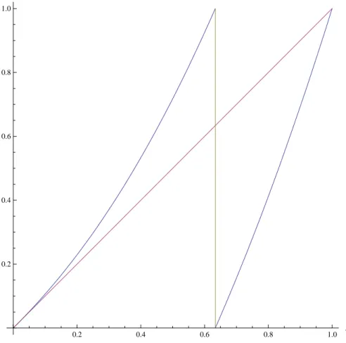
Figure 1.2: Manneville map for z= . α =
Manneville’s Map and Manneville’s distribution
In an article of [] Paul Manneville proposed a model for intermittent turbulence, which we shall call Manneville’s map
yn+= M(yn) = yn+ αyzn (mod ) (.)
withz > . This function is plotted in Figure ..
As Gaspard and Wang found in [] Manneville map dynamic has a very distinctive behavior
≤z ≤
normal dynamics (Gaussian Fluctuations (.)
≤z ≤
transient anomalous dynamics (.)
≤z anomalous dynamics (Lévy fluctuations) (.)
As we see from figure . forz= . dynamics of Manneville model is characterized by a certain form of clustering: long periodlaminar phases interrupted by chaotic burst.
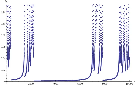
2000 4000 6000 8000 10 000 n 0.02 0.04 0.06 0.08 0.10 0.12 yn Manneville series
Figure 1.3: Manneville series for z = . a = x= .
After establishing the intermittent nature of y we aim to calculate its probability density function [], to do that we have to take a continuous time limit, by example considering the differential equation:
y′= αyz. (.)
the solutions of this equation is given by: α(τ− τ) =
∫
y y yzdy= − z ( yz− − yz− ) . (.) Thus, the time distance between two consecutive jumps (that is, by the structure of ., we sett= and y = ) is given by
ατ= − z ( yz− − ) . (.)
by inverstion of this equation we get:
y= ζ(τ) = (
( − z)ατ + )
/z−
. (.)
Since y∼ U(, ) we have
ψM(t) = d dt Prob(τ < t) = d dt Prob(y< ζ(t)) = d dt ( ( − z)t + ) z− = (µ(T + τ)− )Tµ−µ (.) where we have setµ= z
z− andT =(z−)α .
We can apply Gaspard and Weng analysis [] to this case and obtain:
µ≥ normal dynamics (Gaussian Fluctuations, finite mean and variance) (.) ≤µ ≤ transient anomalous dynamics (finite mean, variance not defined)
(.) ≤µ ≤ anomalous dynamics (Lévy fluctuations, mean and variance not defined)
(.) Thus, Manneville’s intermittency is governed by a power law. We shall see that Laplace Transform (see []) of probability density functions is of fundamental importance for our theory but in this case a closed form is not available. We have, in fact,
ˆ ψM(s) =
∫
∞ e−st(µ − )T µ− (T + τ)µ dt= (µ − )T µ−sµ−e−sTΓ( − µ, sT) (.)where Γ(x, α) =
∫
α∞ettx−dt is the upper incomplete Gamma function []. ψM(t) is a probability density function ˆ(ψ)M() = we can compute his asymptotic behavior for s → and obtainIf < µ < we can expand the function and obtain: ˆ ψM(s) ∼ − Γ( − µ)(sT)µ− (.) IF < µ < we obtain instead: ˆ ψM(s) ∼ + sT − µ −Γ( − µ)(sT) µ−= + s⟨t⟩ − Γ( − µ)(sT)µ− (.)
Lévy function
Lévy’s distribution is another function which can be used as asymptotic power law. Lévy introduced his distribution looking for [, ]
Definition 1.1.1(infinite divisible distributions). Let φX(t) be the characteristic function
of a probability distribution f(t) (i.e φX(t) = Eµ(eiωXwhereX∼ µ). A probability function is said to beinfinitively divisible if for any n there exists a probability measure ν whose characteristic function λn(t) satisfies
φX(t) = (λn(t))n.
Among all the infinite divisible distributions a particular class is of wide interest. To explore this point let us use
Definition 1.1.2(Stable distribution). A distribution is stable if it is stable under
convo-lution that is if, for anya,a,b,bthere exista, b∈ R , so that its characteristic function φX(t) satisfies:
φaX+b(t) = φaX+b(t)φaX+b(t)
If two random variablesXandXare distributed according to a stable distribution the
their sum (rescaled and translated) is also distributed with the same distribution.
The most widely known stable distribution is the Gaussian distribution. Levy and Kin-chine have shown that the only possible attractors of probability distribution are stable distribution and Levy has given a canonical representation theorem
Theorem 1.1.1(Lévy-Kintchine representation theorem). The most general form for the
characteristic function Lα,β(k) of a stable is given by
lnLα,β(k) = iγk − c∣k∣α( − β k ∣k∣ω(k, α)) (.) where ω(k, α) =⎧⎪⎪⎨⎪⎪ ⎩ tan(πα ) if α ≠ πln∣k∣ if α = (.) where γ is arbitrary, c> , α ∈ [, ], − < beta <
Sinceγ and c are scale factors, the do not contribute to the shape of the distribution. α and β instead determines the shape Lévy distribution. The first exponent is called the characteristic exponent since it governs the asymptotic behavior of the distribution, we have in fact
for < µ < The (bilateral) Laplace transform of the distribution can be calculated since
we have the characteristic function and expanding near origin we have Lα,β(is) = ˆψL(s) ∼ − ∣k∣α− β∣k∣α− k ω(k, α) we get that ψL(t) → ± ∣x∣+α forx → ±∞ (.)
for α= the function becomes a Gaussian distribution.
The β is called skewness parameter since it control the symmetry of the function. For β= we obtain symmetric Lévy function, for β = − The distribution in concentrated in the half line[γ, ∞]
1.2 Mesoscopic phenomena and stochastic processes
Phenomena usually studied by physicists have well defined physical scales. Newtonian dynamics, classical (equilibrium) statistical physics and general relativity investigates macro-scopical phenomena in which the fluctuations can be neglected, quantum physics inves-tigates microscopical phenomena in which quantum fluctuations are not negligible any more. Recent advances in technologies (e. g. molecules tracking) have enabled scientists to investigate phenomena whose typical scale are not large enough that fluctuations due to microscopical dynamic can be totally neglected and still not small enough that a complete quantum mechanical treatment can be set up. For these phenomena the name ofmesoscopic phenomena has been proposed.
The natural framework in which those systems are studied is that of stochastic processes. Stochastic processes can be seen as a kind of “microscopical phenomenological description” of the systems, that is, we take into account the microscopical dynamics through a fluctuating variable which describes it “phenomenologically”.
This approach is obviously not new to physics: it has been, indeed, widely used in those fields whichante tempora studied phenomena we could today define as mesoscopic (e.g. non equilibrium statistical physics, Brownian motions etc.). We want to point, nonetheless, that recent advances in experimental techniques have enabled us to study an extremely rich variety of new systems and phenomena which cannot be interpreted from within the usual perspective applied to those disciplines. New “interpretational” paradigm are needed to describe these new fundamental phenomena (and some, like self-organized criticality have yet been provided and have manifestated a powerful exegetic strength ).
1.2.1 Stochastic processes: some definitions
Usual mathematical description of probability is quite cumbersome, under certain aspects. Here we shall limit ourselves to state some definition a property needed further. As a reference books we have mainly used [] and [] (and also [], []).
Definition 1.2.1(Stochastic Process). Let L(X, µ, B) a probability space, a stochastic (or
random) process is collection of stochastic variables{Xt}t∈T parameterized over a setT and
assuming values in Rn
IfT = R then we shall call the process a continuous time stochastic process. If T = N then we shall call the process adiscrete time stochastic process
This definition enables us to translate every concept we already have on stochastic variables to stochastic processes
Definition 1.2.2(Finite dimensional distributions). Given a a stochastic process{Xt}t∈T
over the probabilityL(X, µ, B), for any finite dimensional set of indexes {t
, . . . ,tk} we
define we define the finite dimensional distributions of the process the sets of measures {µt,...,tk(F× ⋯ × Fk)} over R
nkdefined by
µt,...,tk(F× ⋯ × Fk) = Prob(Xt ∈ F∩ Xt ∈ F∩ ⋯ ∩ Xtn ∈ Fn) (.)
The mathematical definition of our process allows us to interpret them in tree different ways: either as random variables (i.e. measurable functions over our probability space Xt ∶ X → Rn) or as functions defined over the setT× X (i.e. instead of interpreting it like
Xt(F) we look at it as X ∶ (t, F) ∈ T × X → Rn). A third possibility is to interpret them as
model functions for physics problems.
Definition 1.2.3(Path). For any Fixed F ∈ B we call the function
fF(t) = X(t, F) (.)
apath of our process.
As usually done for any set of variables, we can define some statistical properties for our processes. Two statistical properties are particularly important :
Definition 1.2.4(Mean). Let{Xt}t∈T be a process on the probability spaceL(X, µ, B),
and let µtthe -dimensional distribution as defined in definition .. We call the function
µ(t) = E(Xt) =
∫
Xtdµt (.)themean of the process and
Definition 1.2.5 (Autocorrelation). Let {Xt}t∈T be a process on the probability space
L(X, µ, B) and let µ
t,s the -dimensional distribution as defined in definition . we
define the function
C(t, s) = E(XtXs) =
∫
XtXsdµt,s (.)theautocorrelation of the process.
Among the great variety of processes a particular class of continuous time processes are very important and are characterized by Markov Property
Definition 1.2.6(Markov Processes). Let{Xt}t∈T be a process on the probability space
L(X, µ, B), We say that the process is a Markov process if, for any set of indexes {t
, . . . ,tk−,s} ∈
R+k so thatt< t< ⋯ < tk−< s the process has the Markov Property
Prob(Xs ∈ Fs ∣ Xt
k− ∈ Ftk−∪ ⋯ ∪ Xt ∈ Ft) = Prob(Xs∈ Fs∣ Xtk− ∈ Ftk−) (.)
Using the definition of conditional probability and definition of finite dimensional distribu-tion we get the previous property translates
µs,tk−,...,t(G × Fk−× ⋯ × F) =
µs,tk−(G × Fk−) ⋅ µtk−,tk−(Fk−× Fk−) ⋅ . . . ⋅ µt,t(F× F)
µtk−(Fk−) ⋅ . . . ⋅ µt(F)
(.) that is the and dimensional distributions totally determines the process.
Ifµt,s(F, G) = µt−s,(F, G) the Markov process will be called time homogenous, otherwise time inhomogeneous.
Since we are interested in modeling physical systems we content ourselves to choosing R as basic space . We, moreover, will assume that the probabilities involved can be expressed in terms of their probability density functions (to be true with a slight abuse of notation we shall consider among those densities also the tempered distributions like Dirac’sδ(t)).
In the following, if nothing is otherwise expressed, we shall indicate the processes simply by Xtor even X(t) where no confusion is possible and the probability density function of our process will be simply denoted like p(x, t) = Prob(Xt ∈ [x, x + dx]). Conditional probability analogously will be written like p(x, t ∣ yt′).
Markov Chains
Among all Markov processes an important class shall be studied more accurately
Definition 1.2.7(Markov Chain). A Markov process{Xt} over a countable (of finite) subset
of R is called a Markov Chain.
Since the possible outcomes the stochastic process can give are countable we shall use a more comfortable notation. We label each possible outcome which we shall refer to asstate, with an integeri and denote the probability of the state i to occur at time t with πi(t).
We will call thetransition probability Wi j(t, s) the conditional probability Prob(i, t ∣ j, s). ObviouslyWi j(t, t) = δi jwhereδi jis the Kronecker symbol.
If Markov property holds we can write πi(t) = ∑
j
Wi j(t, s)πj(s) (.)
It straightforward to derivate some important properties like
Proposition 1.2.1(Chapman-Kolmogorov-Smoluchovski). For all i, j and for all s< u < t
the transition probabilities satisfies
Wi jt, s= ∑ k
Wik(t, u)Wk j(u, s) (.)
We shall show that under certain regularity hypothesis a differential system of equation can be obtained.
Let us assume that Wi j(t + dt ∣ t) = δi j+ Ki j(t) dt + o(dt) and π
i(t + dt) = πi(t) + d
dtπ(t) dt + o(dt
). We can thus write:
d
dtπi(t) dt = ∑j Ki j(t) dtπj(t). (.) If the series ofKi jpj(t) still converge we can take limits and obtain
d
dtπi(t) = ∑j Ki j(t)πj(t),
(.)
which we shall calltime inhomogeneous Master equation.
If the Markov Chain istime homogenous the transition probability will satisfy Wi j(t, s) = Wi j(t − s, ) and thus Wi j(t + dt, t) = Wi j(dt, ).
IfWi j(dt, ) → δi jat least linearly in dt we can take the limit for dt→ and we can write d
dtπi(t) = ∑j Ki jπj(t)
(.)
whereKi j= d
dtWi j(t)∣. Equation . is usually known in physics asmaster equation.
Since πi(t) are probability, we have to request that ∑iπi(t) = for every time. If
d
dt∑iπi(t) = ∑i d
dtπi(t) we have that ∑i∑jKi jπj(t) = . If we change the order of
summa-tion¹ we obtain that theKi j satisfy the request ∑
i
Ki j= . (.)
Under these conditions (Kii= − ∑i≠ jKi j) we thus restate the master equation in the form d
dtπi(t) = ∑j≠iKi jπj(t) − Ki jπi(t).
(.)
The physical interpretation of master equation is now clear. If we interpret the pi as the occupation probability of a statei, Ki jπj(t) measures the occupation growth of state i due to particles that leave the state j to go to the state i, Ki jπi(t) measures, instead, the decrease of occupation of state i due to particles that leave state i to go to state j.
A Markov chain is said to have reachedequilibrium if its probability distribution is time independent.
If our Markov chain satisfies a master equation an equilibrium exists if∑jKi jπj(t) = . If the states are infinite we cannot establish a priori if an equilibrium exists. If we are dealing with a finite state homogenous Markov Chain the existence of equilibrium is guaranteed. We have, in fact, thatKi jare the entries of a matrix K and theπi can be thought as the elements of a vector π. Since equation . says that one raw it a linear combination of the other ones, we have that Ker(K) contain at leat one possible equilibrium solution.
the hypothesis we have made are trivially true for finite dimensional Markov chains
Discrete time Markov Chain
The previous discussion cannot be carried out for discrete time Markov Chains since limits are not allowed. This is not a big deal. We shall repeat our discussion to obtain a similar result.
Probability transition will now depend on to discrete indicesWi j(n, m) with Wi j(n, n) = δi j. In this case Markov Property translates nicely since in the discrete case there is a “last
step before”, that is :
πi(n) = ∑ Wi j(n, k)πj(k) = ∑ Wi j(n, n − )πj(n − ). (.)
We can defineKi j(n − ) = Wi j(n, n − ) − δi jand restate the previous condition as πi(n) = ∑
j (δ
i j+ Ki j(n − ))πj(n − ), (.)
which is the discrete analog of inhomogeneous Master equation.
If the process it finite dimensional we can adopt a vector form that is a matrix(K)i j = Ki j and a vector π(n) whose components are πi(n). The discrete time master equation then become:
π(n) = π(n − ) + K(n)π(n − ). (.)
Thus
π(n) = Π(n)π() (.)
where Π(n) = ∏j(I + K(j)) is called the propagator of the system. For time homogenous discrete Markov Chain we have Π(n) = Π()n.
Coin tossing
Fair Coin tossing may be seen as a Markov Chain. There are only two states, we denote them + and -, and at each step the system can move to the state+ with probability / or in the state− with probability /.
The most general form the operator K fitting the constraint∑iKi j = is
K= ( a b
−a −b). (.)
In order for that the equilibrium to be(/, /) we must set: K= (/ −/
−/ / ). (.)
We notice that K+ K = . We refer to this throughout as a dichotomous process.
Dice throwing
A generalization of previous problem is that of a Markov chain in which the system hask states and at each time moves to one of those state with a given probabilityπk. We call π(n) the vector of probability at timen, πeqthe steady distribution and K the transition matrix previously defined, we have
π() = (I + K)π() = πeq (.)
and
π() = (I + K)π() = πeq (.)
thus yielding the matricial equations:
K+ K = (.)
and
K πeq = (.)
We shall refer to this throughout as multichotomous process.
Random Walk
Another important example of discrete Markov Chain is random walk. In this case we chose our transition probability to be constant and have
Wi j = pδi j−+ qδi, j + with p + q = (.)
The master equation then reads
πi(n) = pπi−(n − ) + qπi+(n − ) (.)
the solution is easily obtainable and has a typical Bernoulli distribution πi(n) = ( n
n− i)piqn−i (.)
1.3 Subordination theory and renewal processes
As we have earlier pointed out, we are mainly interested in systems which exhibit complex behavior characterized by the presence of abrupt transition (which we call “events”) between two or more state, with a power law distribution density of the time distance between two consecutive events.
A benchmark characteristic of those system it ageing, that is the system maintains a memory of the moment of preparation.
The theoretical frame which better suits the description of these systems is that of sub-ordination theory of renewal systems. A substantial treatment of this topic in advanced probability theory can be found in Feller’s work( []and []) and a general review on renewal theory can be found in Cox’ work []
We shall first illustrate Blinking quantum dots behavior as a prototype of the systems we are interested in.
Blinking quantum dots: a prototypical system
Quantum dots (nanocrystals of semiconductors) are intensively studied since they seem to promise great applications like light emissive diodes, solid state lighting, lasers. Investigation on their nature has pointed out some characteristic behavior: fluorescence intermittency [].
This intermittency, subsequently calledblinking, still has a non completely understood microscopical origin (even if many interpretation have been advanced) and constitutes a major problem to be solved to be able to use semiconductors nanocrystals at their best.²
Figure 1.4: A figure taken from [] which shows the typical blinking behavior of quantum dots
The behavior of the blinking is complex; that is, it cannot be described by a poissonian waiting time distribution. As shown in [] this typical behavior cannot be interpreted as a consequence of slow modulation of parameters, since non ageing is possible within the framework of this theory. Renewal subordination theory instead has, as a benchmark, that of showing ageing.
Figure 1.5: A figure taken from [] which shows the typical intensity over time behavior of quantum dots
Figure . shows a typical intensity over time fluctuation of blinking quantum dots. Anal-ysis of those data shows that the permanence time is a random variable which is roughly
recently a possible solution to this problem has been proposed [] but still it does not unveil the nature of this behavior
distributed like∼
tµ.
To model these systems we imagine that the interaction among units has the effect of creating abrupt transitions from one state to another. This is equivalent to assume that the process is modeled by a coin tossing Markov chain. The time between two tossings, due to complex interactions, is not constant any more but is distributed according to a power law.
This is the basic idea of subordination theory and we shall analyze it now.
1.3.1 Subordination theory
We start with a definition
Definition 1.3.1(Subordinated process). Let{Xn} be a discrete time stochastic process
defined over R, and{Tn}n>a discrete time stochastic process defined over R+. We defined
the subordinated process ofXn toTnthe continuous time processξ(t) defines ξ(t) =⎧⎪⎪⎨⎪⎪
⎩
Xift< T
Xn ifTn< t < Tn+
(.)
We shall call{Xn} the leading process and {Tn}n>thesubordination generating process. We want to point out that this is amathematical model. The only physical process is the result of subordinationξ(t) and both the leading process and the subordination generating process are phenomenological description of collective interaction.
Surely in certain cases we can give the leading process a microscopical interpretation, like the modeling of shocks in a ideal gas if we accept Boltzmann’s Stosszahlansatz. The waiting time distribution, in this case, will have to be inferred from the statistical properties of ideal gases.
Complex phenomena do not allow, usually, such a simple interpretation in terms of local microscopical vs. global macroscopical behavior, since both processes involved in subordination structure emerge from cooperative global interactions. The distinction is rather made in term of the effects both processes give rise to (i.e. the distinction we make is ana posteriori phenomenological one that enables us to propose a model).
Another fact that should be stressed is that subordination is a key mechanism to explore cooperative systems which could also not be simple fundamental physical systems. Studies in neural and social network have shown to exhibit this characteristic behavior (which happens to be tunable moreover).
Independent Increment Processes and renewal processes
The previous definition is rather general. We could choose assubordination generating process an arbitrary one. The first simplification we shall make is that of considering :
Definition 1.3.2(Independent increment processes). A stochastic process{Xt} is said
to be anindependent increment process if for any s < t < w < u Xt− Xs and Xu− Xw are independent variables.
The previous condition implies that the probability density function of the interval de-pends only on the time difference (i.e. Prob(Xt− Xs ∈ [x, x + dx]]) = f (x, t − s)). Among all independent increment processes we are particularly interested inrenewal processes
Definition 1.3.3(Renewal process). A discrete time independent increment process{Tn}
defined on R+is called arenewal process
The reason why this kind of processes are called renewal processes will be clarified in next section. We first point out the most important property of those systems.
A renewal process{Tn} is totally determined by only one distribution
ψ(t) = Prob(Tn+− Tn ∈ [t, t + dt]) = Prob(T− T∈ [t, t + dt]) = f (t, ) (.)
which in the contest of subordination theory we shall callwaiting time distribution.
The independent increment process condition enables us, in fact, to obtain all the other conditions immediately. If we define the events
A(t, n) = {Tn− T∈ [t, t + dt]} (.)
by the independent increment hypothesis those events are independent. In particular the event A(t, n) can be split recursively in this way:
A(t, n) = ⋃
t′ [A(t − t
′, ) ∩ A(t′,n− )], (.)
that is, we consider the probability of having the n-th element in[t, dt] as probability to find then− -th in t′ < t and that last interval has the length t − t′(obviously this works
becauseTn ∈ R+) we immediately write
ψn(t) = Prob(A(t, n)) = Prob(⋃ t′[A(t − t ′, ) ∩ A(t′,n− )]) =
∫
t ψn−(t′)ψ(t − t′) dt′. (.) If we consider the Laplace transform (for the mean properties look Appendix) of the waiting time distribution ˆψ(u) the Laplace transform of ψn(t)ˆ
ψn(u) = ˆψn(u). (.)
Renewal hypothesis: waiting time distribution as renewal failure time distribution
To clarify why discrete time positive valued independent increments processes are called renewal processes we have to think waiting time distribution as a failure time distribution. In its classical Monograph on Renewal Theory ( []) Cox gives a simple but insightful description of what a renewal process is.
Renewal theory is originally linked to the study of probabilistic problems connected with the failure and replacement of components. typical terminology could sound a little weird to a scientist’s ear, but we shall use it, for now, to let reader to easily find it in specialistic literature.
Let us then think to a robotized assembly line. It will work efficiently if all its components are working. But even the best constructed robot will endure soon or later some failure problems (due to wear e.g.). We now think that every time a robot fails it is immediately and completely restored in a perfectly working state. This is called therenewal hypothesis
For simplicity sake (and we are actually interested in these kinds of mechanism) we consider a single robot line.
We can model the failure probability of these robots as real positive random variable T called failure time. This failure time give rise to a failure time distribution f(t). The probability for the system not to break if calledsurvival probability and has the obvious expression
Ψ(t) = Prob(T > t) =
∫
∞
t f(t
′) dt′. (.)
We can construct a discrete time process setting{Tn} is the time of the n-th failure and renewal. This is, by construction, a discrete time positive values independent interval process as previously defined and now the reason why it’s calledrenewal process is clear.
Renewal hypothesis make us able to give a nice description of failure time distribution f(t)
Let us consider a key property of renewal processes calledfailure rate:
g(t) = lim
∆t→+
Prob(T ∈ [t, t + ∆t]∣t < T) ∆t
. (.)
Since Prob(T ∈ [t, t + ∆t]∣t < T) = Prob((T∈[t,t+∆t])∩T>t)
ProbT>t we get g(t) = f(t) Ψ(t). (.) By definition Ψ(t) = −d dtf(t). Therefore: g(t) = −Ψ′(t) Ψ(t) = − d dt log Ψ(t) (.)
integrating equation . and noticing that Ψ() = , we obtain Ψ(t) = exp(−
∫
t
g(t′) dt′). (.)
Therefore, a renewal-process occurrence time is completely characterized by its failure rate. Equation . enables us to make some analysis on g(t).
• g(t) = in this the mean failure rate is constant and we obtain Ψ(t) = exp(−gt) and subsequently f(t) = g exp(−gt): this is the case of Poissonian failure time distribution. This is the typical “ failure” mechanism in traditional physics (e.g. radioactive decay, usual statistical physics phenomena etc.)
• g(t) ∼ Atαwith α> In this case we get a probability whose queues are super
exponen-tially depressed∼ exp−Btα+/(α + )
• g(t) ∼ A ∗ tαwith < α < In this case we get sub exponential distribution which
asymp-totically give rise to what are called stretched exponentials distribution Ψ(t) ∼ exp(−Atγ/γ) withα+ = γ ∈ [, ]
• g(t) ∼ A/t In this case we get power laws in fact Ψ ∼ exp log(t−A)) = tA
• g(t) ∼ tα with α< − In this case we find the construction is impossible since it would
lead to immortality that is the f(t) is not normalized to
This analysis shows than that the power laws are a limiting case of failure time distributions that seem to correctly modelsporadicity.
We notice, moreover, thatg(t) is not constant so the failure rate, that is the probability of decaying, changes over time: the system is ageing in the sense that from an estimationg∗ ofg(t) we can get an estimation of the age (i.e. the time elapsed since last failure) of the system g−(g∗)
Specific choice of g(t) let us to derive the power laws we have already presented. If g(t) = r
+rt
we obtain Ψ(t) = (r+ t)−r/r. If we callµ = − r r
and T = rwe obtain back Manneville’s distribution ..
More complicated (i.e. non analytical) choices lead to Lévy and Mittag-Leffler distribu-tions.
The rate of event per unit time
Let us consider the random variable
N(t) = # events occurred in [, t] (.)
we may ask what is the mean number of event. This calculation is easily carried out if we notice that the probability of having n events before timet that is B(n, t) = {n events have occurred before time t} can be split using using .
Prob(B(n, t)) = Prob(⋃ t′(A(n, t ′) ∩ A(, t′)) =
∫
t ψn(t − t′)Ψ(t′) dt′ (.)and thus the mean is easily written out: H(t) = E(N(t)) ∑ n n Prob(B(n, t)) =∑∞ n=
∫
t nψn(t − t′)Ψ(t′) dt′ (.)Using Laplace transform we have :
H(u) = − ˆψ(t) u ∞ ∑ n=
∫
t n ˆψn =− ˆψ(u) u ψ(u) d d ˆψ(u) ∞ ∑ n= ˆ ψn(u) = u ˆ ψ(u) − ˆψ(u) (.) and thus H(t) =∫
t ∞ ∑ n= ψn(t′) dt′. (.) We can now define a crucial quantity for our renewal processesmean rate of events : R(t) = d dtH(t) = d dtE(N(t)) = ∞ ∑ n= ψn(t) (.)
Another way to understand what R(t) is, can be that of considering the event E = { an event occur at time t }. In can be easily be split into an union of independent event that is
Prob(E) = Prob(⋃
n
A(n, t)) dt =∑∞
n=
ψn(t) dt = R(t) dt. (.)
For Manneville power law, using Tauberian Theorem and asymptotic expansion . and . we write for < µ <
R(u) ∼ (uT)−µ Γ( − µ) (.) and thus R(t) ∼ Tµ−Γ( − µ)Γ(µ − ). (.) and for < µ < R(u) ∼ ⟨t⟩u + (uT) −µ Γ( − µ) (.) and thus R(t) ∼ ⟨τ⟩[+ Tµ− − µ tµ−]. (.)
Subordinated renewal processes
We can now completely analyze subordinate renewal processes. Our analysis is based on the seminal works of Montroll and Weiss on Continuous Time Random Walk (CTRW) [] .
Our end is to obtain the the distribution of the subordinated processπ(ξ, t).
The key idea is to consider that according to our definition, the to processes are indepen-dent. Since we know by hypothesis the distribution of the leading process p(x, n) and our waiting time distribution we have everything. In fact the pdf
p(ξ, t) dξ = Prob[(X∈ [ξ, ξ + dξ] ∩ no event occurred until t) ∪ ⋯
∪(Xn∈ [ξ, ξ + dξ] ∩ exactly n events occurred before timet ∪ ⋯]
(.) Since, by independence we can write
p(ξ, t) dξ = Prob(⋃
n (B(n, t) ∩ Xn ∈ [ξ, ξ + dξ) = ∑n
Prob(B(n, t))π(ξ, n) dξ (.) Now we have all the pieces of information needed to write (which sometimes known as Montroll-Weiss equation) p(ξ, t) = ∑∞ n=
∫
t ψn(t − t′)Ψ(t′)π(ξ, n) dt′. (.)This is the most general form Montroll-Weiss equation can take unless we make some other hypothesis on our system.
Generalized master equation
If{Xn} is a finite time homogenous discrete Markov Chain, adopting our shortcut notation ³ we can write: p(t) = ∞ ∑ n=
∫
t ψn(t − t′)Ψ(t′)Π()ndt′π(). (.)Taking the Laplace transform of both sides we write:
ˆ p(u) = − ˆψ(u) u ∞ ∑ n=(ψ(u)Π()) ndt′π(). (.)
Since both∣ ˆψ∣ and ∥Π()∥ are less than we can sum the geometrical series and considering that p() = π(), we have: ˆ p(u) = − ˆψ(u) u − ˆψ(u)Π()p(). (.)
Defining K= Π() − I and rearranging we obtain: uˆp(u) − p() = u ˆψ
− ˆψ(u)
K ˆp(u). (.)
Transforming back we obtain theGeneralized Master Equation d
dtp(t) =
∫
t
Φ(t − t′)Kp(t′) dt′, (.)
where the quantity Φ(t) is called memory kernel and is defined by its Laplace transform: ˆ
Φ(u) = u ˆψ(u)
− ˆψ(u). (.)
We thus see that subordination induces a loss of Markoviantity, that is, it introduces memory in the process.
Ageing
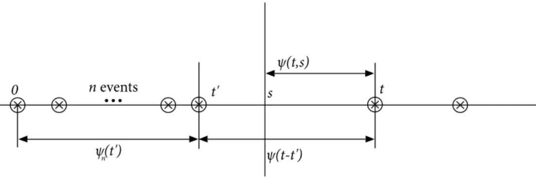
Renewal processes by derived by subordination are characterized by ageing. To see it let us suppose a renewal system is prepared at time , and our observation starts at times. Obvi-ously the first occurrence time is no more governed by our waiting time distribution. We have in fact (a graphical sketch can be found in picture .) to find the distribution the eventO= { the first observable event occur at time t given the system observation started at times}.
As usually we can split, for any (< t′< s < t this event as follows:
O= ⋃
t′ ⋃n (A(n, t
′) ∩ A(, t − t′)) (.)
we label states byj and consider the probability vector π(n) of π( j, n) and the vector p(t) of the probability p(i, t)
0 t' -t's t ψ(t-t') ψ(t,s) n events n
...
ψ(t')nFigure 1.6: A visual sketch of aged waiting time calculation
that is, by disjunction and independence we can write thewaiting time distribution of age s:
ψ(t, s) = Prob(O) =∑∞ n=
∫
s ψn(t′)ψ(t − t′) dt′= ψ(t) +∫
s R(q)ψ(t − q) dq. (.) We can associate thesurvival probability of age s integrating :Ψ(t, s) =
∫
∞ t ∞ ∑ n=∫
s ψn(t′)ψ(t′′− t′) dt′dt′′. (.)Changing the order of integration and using formula . we obtain:
Ψ(t, s) = Ψ(t) +
∫
s
R(t′)Ψ(t − t′) dt′ (.)
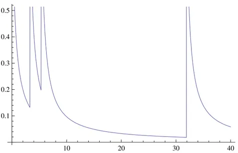
We can obtain directly this prescription considering the stochastic failure rate that is :
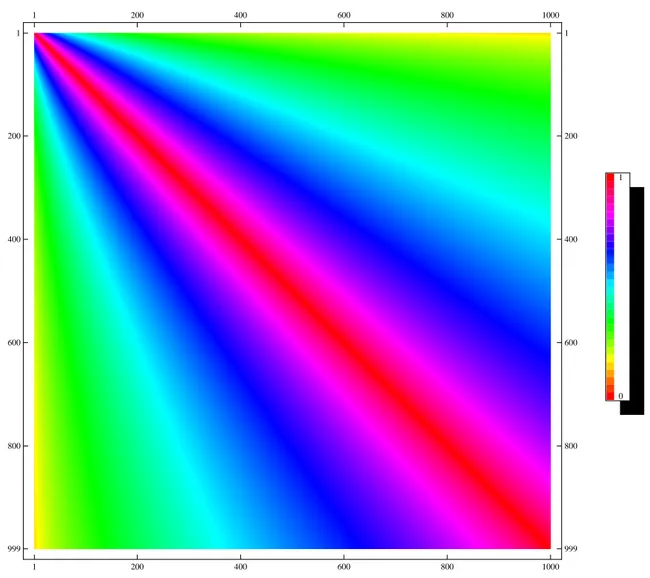
r(t) = g(t − ti) (.)
In a certain wayr(t) represents the failure rate of the entire process see figure . Remembering the definition of g we can write:
Ψ(t, s) = ⟨
∫
s δ(q) + R(q)e−∫qsr(τ) dτ ⟩ =∫
s (δ(q) + R(q))e −∫qsg(τ) dτdq= Ψ(s) +∫
s R(q)Ψ(t − q) dq (.)We want to point that for poissonian processes we have g(t) = r(t) = R(t) =
⟨t⟩ (.)
10 20 30 40 0.1 0.2 0.3 0.4 0.5
Figure 1.7: A simple example of r(t) corresponding to equation g(t) = +t
non stationarity
The aim of this chapter is to introduce the reader to the concept of ergodicity as it has been conceived by physicists and mathematicians and to analyze some physical phenomena which exhibit an “ ergodicity breaking’. It will be shown, in particular, that complex systems are likely to be considered “non ergodic systems”
2.1 Boltzmann’s Ergodic hypothesis
Theory of “irreversibility’ had always been a hard problem to deal with for physicists of XIX century. Clausius law, which had been proved by experiments, posed ha complicated problem. How can irreversibility arise from fundamental microscopical laws, which are time invariant?
It was not until the end of the century that a solution appeared, thanks to the work of Boltzmann.
Ludwig Boltzmann had yet began to organize his theories about irreversibility while building his kinetic theory. His H functional seemed, then, to provide a good mathematical instrument to show that irreversibility could be outputted by his kinetic theory but still he wasn’t able to link his “phenomenological’ theory to microscopical fundamental laws.
During the ’ and ’ of XIX century Boltzmann in his papers proposed hisErgodic Hypothesis as the foundations of his, then innovative, theory of irreversibility. The usual form under which ergodic hypothesis is stated nowadays is to be ascribed to Ehrenfest, who in a review of [], stated it :
Boltzmann-Ehrenfest’s Ergodic hypothesis A dynamical system during his evolution
will takeall the microscopical configurations compatibles with a given macroscopic state (i.e. a single trajectory will cover the whole phase space during his evolution) To be true Boltzmann never stated his hypothesis this way, but he limited himself in assuming a “uniform probability“ of phase space.
Conservative systems’ evolution is known to follow Liouville’s equation
∂tρ= L ρ (.)
whereρ(pi,qi) ∏idd piddqi is the measure on the phase space (MPS).
Liouville’s theorem warrants us that time evolution preserves phase space measure. Nor-malizing MPS we get a probability space. Thus for conservative systems, this probability is
invariant under time evolution. This mean that we can ”safely“ considertemporal means of a variable f : lim t→∞/t
∫
t f(x(t)) dt (.)Under Boltzmann-Gibbs frame, we “introduce” a measure of our ignorance of the effective initial conditions of the system by defining a new space, theGibbs ensemble, which is nothing but the set of infinite copies of the given dynamical system at fixed time, each one of which is the time evolute of one of all the possible compatible initial conditions. We associate a probability measure to each phase space configuration in the usual frequency limit way and use it to calculate averages.
Ergodic hypothesis is, roughly speaking, nothing but the assumption that MPS and Gibbs measure are the same that is, temporal mean and Gibbs average are the same.
As stated earlier, Boltzmann-Ehrenfest Hypothesis is proved to be false. The original Boltzmann hypothesis as been weakened and stated in a more “realistic” way:
Ergodic hypothesis (weak form) The set of values taken by a dynamical system is dense
in the set ofall the microscopical configurations compatible with a given macroscopic state.
Under this form, which has enabled mathematician to state and prove ergodic theorems, Ergodic hypothesis has been proved to hold for some dynamical systems but it is still not clear why it should be true for all. Moreover if warrants the existence of time and ensemble averages and their equivalence it has been shown that for an arbitrary observable the time needed to reach equilibrium is exponential in the number of elements of the system.
Most authors (i.e. Landau [] ) tend to diminish the importance of this hypothesis as a foundational hypothesis of Statistical physics and in recent years many examples of ergodicity breaking has been shown to exist.
We will show that the complex systems of our interest are non ergodic.
2.2 Mathematical theory of ergodicity and Brickhoff
theorem
Mathematicians have tried to establish a well founded theory of ergodicity, during the XX century and have succeeded in establishing very powerful results, which are linked to mathematical theory of dynamical systems. Before correctly stating the main, and most known result of this theory, we have to give some preliminary definitions (see also []).
As we have shown in the previous chapter, Boltzmann’s ergodic hypothesis allows us to associate to any system a probability space L(X, B, dµ) which describes how certain
microscopical configurations lead to a given macroscopical configuration. In this theory the macroscopical value of adynamical variable A is calculated as the mean⟨A⟩ =
∫
A dµ.Traditionally a statistical dynamical system is described mathematically by a flow from a metric space to another
Definition 2.2.1. Flow Let X be a metric space, we define a flow over X a collection of maps
{Tt∶ Tt∶ X → X} indexed over a given set I such that:
i. TtTs = Tt+s ii. T=
Generically mathematicians callergodic any asymptotic property of a dynamical system expressed by a flow. To find any connection with the main problem of statistical physics we confine ourselves to considertemporal means of dynamical variable f (i.e. a Lfunction of
dynamical variables)
The mathematical ergodic theory aims to analyze the temporal mean
¯ f = lim T→∞ T
∫
T f(Ttx) dt (.)and its relation withspacial mean
⟨f ⟩ =
∫
∞
f dµ (.)
One of the most fundamental question of mathematical theory of ergodicity is to assess when the temporal mean of f is equal to its space mean.
2.2.1 Invariant Measure
Before we continuing our discussion we have to consider some definitions
Definition 2.2.2 (Invariant measure). Let L(X, B, dµ) be a probability space. Then a
measure is said to beinvariant with respect to the flow T ∶ X → X if µ(A) = µ(T−A)
An obvious characterization of invariant measure is the following :
Lemma 2.2.1. A map T preserves µ if and only if
∫
f dµ=∫
T○ f dµ for all in L(X, (B), µ)A trivial generalization of the previous definitions can be obtained for flows
Definition 2.2.3 (Invariant measure). Let L(X, B, dµ) be a probability space. Then a
measure is said to beinvariant with respect to the flow Ttfor t inI if µ(A) = µ(T− t A) for
all t inI
From now on we shall considerI = N and so Tn = Tn. Obviously if a temporal mean exists we can confine ourselves to consider discrete flows. In this case invariance for flows is simply T invariance.
Let us state one of the most fundamental results of ergodic theory:
Theorem 2.2.1(Poincaré Recurrence Theorem). Let T∶ X → X be a measurable
transfor-mation on a probability space L(X, B, µ) preserving µ. Let A ∈ B so that µ(A) > ; then for
almost all points x ∈ A the orbit {Tnx}
n≥returns to A infinitely many often
Proof. Let us define the set
F = {x ∈ A ∶ Tnx /∈ A, n > } (.)
First we note that T−nA∩ T−mA = ∅, for n > m. Where it not, we would have for w ∈ T−nA∩ T−mA , Tmw ∈ F and Tn−m(Tmw) ∈ A contradicting our hypothesis. We can
thus write
∑
n
µ(T−nF) = µ(∪
nT−nF) ≤ (.)
butµ is T-invariant and so equation . can hold only if µ(F) =
2.2.2 Ergodic measures and Birkhoff’s theorem ergodic and invariant
version
A stronger property is needed to establish Birkhoff theorem
Definition 2.2.4 (Ergodic measure). Let L(X, B, dµ) be a probability space. Then a
measure is said to beergodic with respect to T ∶ X → X if for every set B ∈ B with B = T−B,
µ(B) = o µ(B) =
As previously we can characterize ergodic measure in a simple way
Lemma 2.2.2. A map T is ergodic with respect to µ if and only if for every f ∈ L(X, B, µ),
f = T ○ f implies f be constant.
Now we can state the first version of Birkhoff theorem
Theorem 2.2.2(Birkhoff theorem). Let f ∈ L(X, B, µ). If µ is ergodic then
lim N→∞ T N ∑ n= f(Tnx) =
∫
f dµ (.)for almost every x in X
This demonstration is quite technical and not very significant on a pysical point of view. Assuming without loss of generality that
∫
f dµ= , if it is not so we can substitute f withf −
∫
f dµ. The main idea of this demonstration is to show that the set defined: Eε(f ) = {x ∈ X ∶ lim sup N→∞ N ∣ N− ∑ n= f(Tnx) ∣≥ ε} (.)has null measure (i.e. µ(Eε(f ) = ). We first prove two sublemmas
sublemma 2.2.2.1. µ(Eε(f )) ≤ inf ∣f ∣dµε
Proof. Defining f = f+− f−where f+(x) = max(f (x), ) and f− = max(−f (x), ).
Obvi-ously∣ f ∣= f++ f−. Now we define EM ε (f+) = {x ∈ X ∶ ∃ ≤ N ≤ M, N− ∑ n= f+(T nx) ≥ εN} (.) and EM ε (f−) = {x ∈ X ∶ ∃ ≤ N ≤ M, N− ∑ n= f−(T nx) ≥ εN} (.) forM≥ . If we consider that: P− ∑ n= f+(T nx) ≥ εP−M ∑ j= χEM ε (f+)(T jx) (.) and P− ∑ n= f−(T nx) ≥ εP−M ∑ j= χEM ε (f−)(T jx) (.)
where we have bounded f from below by or ε. Thus, integrating both sides of . and .,we write:
∫
P−∑ n= f+(T nx) dµ(x) = P∫
f+dµ≥ ε(P − M)µ(E M ε (f+)) (.) and analogously:∫
P−∑ n= f−(T nx) dµ(x) = P∫
f −dµ≥ ε(P − M)µ(E M ε (f−)) (.) for allM≥ . WhenP→ ∞ we have:∫
f±dµ≥ εµ(E M ε (f±)) (.) and thus µ(Eε(f ) ≤ lim sup M→∞ µ(EM ε (f+)) + lim sup M→∞ µ(EM ε (f−)) ≤∫
f+dµ+∫
f−dµ. (.)Now we need to be able to control the size of the higher bound and to do this we can we prove this second lemma
sublemma 2.2.2.2. If
∫
f dµ= , then, for every δ ≥ there exists a function h ∈ L∞(X, B, µ)for which
∫
∣ f − (hT − h) ∣ dmu < δProof. Let S be defined by: S= {h ○ T − h ∶ h ∈ h ∈ L∞(X, B, µ)} (.) and theB B= {f ∈ L (X, B, µ) ∶
∫
f dµ= }. (.). We first show thatS is dense in B. Hann Banach theorem guarantees us we only need to show that every null functional onS is also a null functional on B.
As known for every functional α(f ) defined on L(X, B, µ), there exists a function
k ∈ L∞(X, B, µ) so that α(f ) =
∫
f ⋅ k dµ Now let us suppose that α vanishes on S thus∫
(h ○ T − h) ⋅ k dµ = if h = k we have k ⋅ (kT)k =∫
kdµWe can then write:
∫
(k○T−k)dµ=
∫
(k○T)dµ+∫
kdµ−∫
(k○T)k dµ = (∫
kdµ−∫
(k○T)⋅k dµ) = (.) We have thatk = k ○ T and so k must be constant by ergodicity hypothesis. We can thus write = k∫
f dµ=∫
f k dµ = α(f ) which proves the lemma.We can now proceed to prove Birkhoff theorem.
Birkhoff ’s theorem proof. As earlier done, we consider without loss of generality f ∈ B.
Let delta > . Using sublemma ... and choose h so that
∫
∣ f − (hT − h) ∣ dµ ≤ δ. Eε(f ) = Eε([f − (hT − h)] + (hT − h)) ⊂ Eε/(f − (hT − h)) + Eε/(hT − h)) and so:µ(Eε(f )) ≤ µ(Eε/(f − (hT − h))) + µ(Eε/(hT − h))). (.)
But∀x ∈ X we can write N ∣ N− ∑ n=(hT − h)(T nx)∣ = N ∣h(T Nx) − h(x)∣ ≤ ∥h∥∞ N (.) and soµ(Eε/(hT − h)) = . Using ... we have µ(Eε/(f − (hT − h))) ≤
∫
∣f − (hT − h) dµ∣ ε/ ≤ δ ε and thusµ(Eε/(f − (hT − h))) = which proves the result.2.3 Ergodicity of time series
It is a well known fact that Dynamical Systems like those considered in the previous section are in fact Markov Chains (see []).
In a certain way the Markov Chain perspective is nothing but a microscopical phenomeno-logical description of the effect of global dynamic of the system. Under this perspective we wonder how ergodicity is espressed in stochastic Process.
In the previous sections we have seen that ergodicity is roughly equivalent to say that the temporal means equal statistic means. Thus a single process we can express ergodicity as follows (see []):
Definition 2.3.1(Strict ergodic process). A stochastic process is ergodic if all his statistical
means can be calculated trough a single realization of the process
as above we can confine ourselves to considering a weaker form of ergodicity that is
Definition 2.3.2(Wide sense ergodic process). A stochastic process is ergodic in the wide
sense if if holds: ¯ Xt= lim T−>∞ T
∫
T −T X(t ′) dt′= E[X(t)] (.) and RXX(τ) = lim T−>∞ T∫
T −TX(t ′)X(t′+ τ) dt′= E[X tXt+ τ] (.)It is natural to wonder what is the equivalent concept of invariance in the language of stochastic processes. In this case too, little work is needed to translate concept:
Definition 2.3.3 ((Strictly) Stationary processes). A random process {Xt} is called a
(Strictly) Stationary process if his cumulative distributions
FXt...Xtn(xt. . .xtn) = FXt +τ...Xtn+τ(xt. . .xtn), (.)
for allti,τ∈ R
Usually weaker form of stationarity is required to get useful results, that is only the first and the second moment are stationary:
Definition 2.3.4(Wide sense Stationary processes). A random process{Xt} is called a
(Weak) Stationary process if its mean
E[Xt] = E[Xt+τ] = µ (.)
and its auto covariance (or autocorrelation)
E[XtXt+τ] = E[XXτ] = C(τ) (.)
For allt, τ∈ R
In a stationary process, thus, we can begin an observation at any time and we shall still be able to access to all the information on the process.
As shown in the previous chapter, ergodicity is a stronger property than invariance: the same holds for ergodic and stationary processes.
Proposition 2.3.1. Ergodicity in the wide sense implies stationarity in the wide sense
Proof. The proof is almost trivial. In fact the limit exists equation . reads E[X(t)] = lim T−>∞ T
∫
T −TX(t ′) dt′= µ (.) and . reads E[XtXt+ τ] = lim T−>∞ T∫
T −TX(t ′)X(t′+ τ) dt′= R XX(τ). (.)Thus proving that a process (or a dynamical system)is not stationary is the same as showing that it is not ergodic.
But stationarity does not imply ergodicity. To see it letU a random variable with mean µ. Let us consider the process defined as follows:
Xt=⎧⎪⎪⎨⎪⎪
⎩
U ift= X ift>
. (.)
By construction this is a stationary process but it is clearly non ergodic. In fact⟨Xt⟩ = µ but ¯Xt= U.
2.4 Ergodicity breaking
When coming to “Ergodicity breaking ” many physicists think to usual critical phenomena. Second phase transition have, in fact, have provided very rich experimental ground upon which physicists have built a very well founded theory (see []). Typically, in those systems, ergodicity breaking is explained as a consequence ofspontaneous symmetry breaking at a certain critical temperatureTc(e.g. Curie Law for magnetization).
Similar but slightly different systems are those which undergo critical dynamics. In this case the system is thought to be in a non equilibrium state and expected to regress to equilibrium during his time evolution. In a totally ergodic system regression to equilibrium should occur with a precise an fixed “mean regression time” which is nothing but the “time correlation length”.
When the system is near a critical point this happens to be false and the more the system is near the critical point, the more the “time correlation length” of the system grows: system exhibit what is calledcritical slowing down.
Yet the simple and rough Van Hove model [] had shown it , and the models further pro-posed by Kawazaki in the late sixties [] and to the work of Höhenberg and Halperin [] [] who managed to give a Renormalization Group description of critical dynamics have con-firmed it.
All these theories have shown that the typical characteristic behavior of a system near a critical point satisfies what is calleddynamical scaling hypothesis, that is, the typical time behaves like:
![Figure 1.1: A figure taken from [?] which shows the emergence of a power law distribution for real networks](https://thumb-eu.123doks.com/thumbv2/123dokorg/7343058.92216/10.892.198.717.623.833/figure-figure-taken-shows-emergence-power-distribution-networks.webp)
![Figure 1.4: A figure taken from [] which shows the typical blinking behavior of quantum dots](https://thumb-eu.123doks.com/thumbv2/123dokorg/7343058.92216/23.892.239.625.291.483/figure-figure-taken-shows-typical-blinking-behavior-quantum.webp)