Scuola di Ingegneria Industriale e dell'Informazione
Corso di Laurea Magistrale in Ingegneria Chimica
3D IMMERSIVE DYNAMIC SIMULATION:
THE AG2S™ PROCESS CASE
Relatori: Prof. Flavio Manenti, Prof. Simone Colombo
Correlatore: Dr.- Ing. Erik Esche
Tesi di Laurea Magistrale di:
Filandro Amoroso
Matr. 833674
A coloro i quali han sempre creduto in me, a tutti i docenti che hanno arricchito il mio bagaglio personale di conoscenze e competenze, ma anche insegnato importanti lezioni di vita. In particolare ai miei relatori di tesi, i professori Colombo e Manenti, che hanno creduto in me permettendomi di collaborare ad un progetto ambizioso ed interessante, ricco di nuove sfide e competenze da acquisire, offrendomi anche la possibilità di realizzare parte del lavoro in un’università estera, un’avventura da me tanto desiderata in passato ed ancor più apprezzata ora che si è conclusa. Un ringraziamento anche ad Erik Esche, persona fantastica che ha reso il mio lavoro alla TU Berlin fruttuoso e stimolante. Infine, un ringraziamento a tutta la mia famiglia che mi ha permesso di realizzare il mio sogno di bambino, quello di conoscere il mondo attraverso le sue leggi.
INDEX
INDEX ... 1
FIGURE INDEX ... 5
TABLE INDEX ... 10
ABSTRACT ... 11
1. IMMERSIVE DYNAMIC SIMULATION: instruments and goals ... 13
1.1 HOW TO CREATE AN IMMERSIVE DYNAMIC SIMULATION ... 14
1.1.1 Intergraph® Smart3D ... 15
1.1.2 Simsci™ Dynsim ... 15
1.1.3 MOSAIC ... 16
2. THESIS OBJECTIVES AND FUTURE STEPS ... 17
3. 3D MODELING: INTERGRAPH® SMART 3D ... 21
3.1 SMART 3D WORKSPACE ... 21
3.1.1 Task grid ... 22
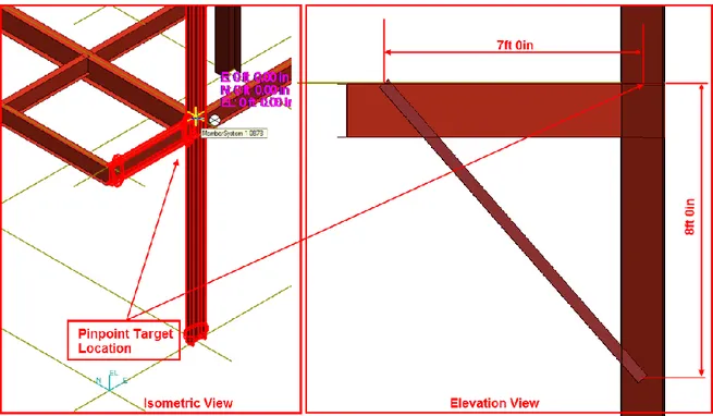
3.1.2 PinPoint ... 23
3.1.3 Structural System task ... 24
3.1.4 Equipment task ... 25
3.1.5 Piping task ... 27
3.2 SMART 3D MODELING OF THE LABORATORY ... 28
3.2.1 Preliminary studies ... 29
3.2.2 Structural system realization ... 31
3.2.3 Equipment realization ... 31
3.2.4 Piping realization ... 38
3.2.5 3D model complete ... 41
4. BEFORE PROCESS SIMULATION: REACTION KINETIC ... 45
4.1.1 Goal of the process ... 45
4.1.2 Reaction description ... 46
4.2 THEORETICAL RESULTS: DSMOKE ... 46
4.2.1 How to find kinetic data ... 46
4.2.2 DSmoke introduction ... 47
4.2.3 DSmoke general features of the kinetic model ... 48
4.2.4 The reactor models and AG2S™ operating conditions ... 51
4.2.5 DSmoke results ... 52
4.3 SIMPLIFIED KINETIC SCHEME FOR SIMULATIONS ... 59
4.3.1 Reasons and structure of the simplified kinetic scheme ... 59
4.3.2 Regression code: C++ and BzzMath© library ... 60
4.3.3 Regression code: manage DSmoke using C++ ... 62
4.3.4 Regression results ... 69
5. DYNAMIC SIMULATION SOFTWARE: DYNSIM ... 80
5.1 STEADY STATE VS. DYNAMIC SIMULATION ... 80
5.2 LABORATORY MAIN COMPONENTS ... 81
5.2.1 Sources ... 81
5.2.2 Fluximeters ... 81
5.2.3 Reactor and furnace ... 83
5.2.4 First trap: sulfur recovery unit ... 84
5.2.5 Second and third traps: H2S removal ... 85
5.3 DYNSIM™ WORKSPACE ... 86
5.3.1 Workspace components: Unit of Measure and Chemistry ... 86
5.3.2 Workspace components: Icon Palette ... 88
5.3.3 Workspace components: Instance tree ... 90
5.3.4 Workspace components: Engineer toolbar ... 91
5.4.1 First section: before reactor components in Dynsim ... 92
5.4.2 Reactor section introduction ... 96
5.4.3 Initial reactor design: PFR in Dynsim ... 96
5.4.4 Complete reactor design: PFR in Dynsim ... 97
5.4.5 Last section: post reactor equipment ... 101
5.5 COMPLETE PROCESS SCHEME AND RESULTS IN DYNSIM ... 105
6. MOSAIC: A NEW MODELING, SIMULATION AND OPTIMIZATION ENVIRONMENT ... 111
6.1 INTRODUCTION OF MOSAIC ... 111
6.2 DISCOVER THE POTENTIAL OF MOSAIC IN IMMERSIVE SIMULATION 112 6.3 REPLACING PROCESS WITH MOSAIC: SIMULATION ENVIRONMENT 113 6.3.1 MOSAIC environment: general overview ... 114
6.3.2 MOSAIC environment: notation ... 116
6.3.3 MOSAIC environment: equations ... 118
6.3.4 MOSAIC environment: interfaces ... 118
6.3.5 MOSAIC environment: connectors ... 119
6.3.6 MOSAIC environment: ports and streams ... 119
6.3.7 MOSAIC environment: equation systems ... 120
6.4 AG2S™ PROCESS IN MOSAIC ... 121
6.4.1 The reactor in MOSAIC ... 121
6.4.2 Reactor model evaluation ... 127
6.4.3 Reactor model results ... 131
6.4.4 Reactor model: discretizing the equation system ... 135
6.4.5 Natural cooling before the first trap ... 142
6.4.7 The second and third traps in MOSAIC ... 148 6.4.8 Building the complete process in MOSAIC: creating ports ... 154 6.4.9 Building the complete process in MOSAIC: connecting ports with streams
161
7. RESUME AND FINAL CONSIDERATIONS ... 167 REFERENCES ... 170
FIGURE INDEX
Figure 1 – Smart3D home screen ... 21
Figure 2 – radial grid ... 22
Figure 3 – rectangular grid ... 22
Figure 4 – example of PinPoint command usage to create a complex beam structure ... 23
Figure 5 - structural system editor bar ... 24
Figure 6 – example of structural system application with the presence of grids... 24
Figure 7 – example of vertical vessel equipment ... 25
Figure 8 – example of designed equipment with preview ... 25
Figure 9 – shapes catalog with preview... 26
Figure 10 – complex piping example ... 28
Figure 11 – plant of the laboratory realized in Autocad® ... 30
Figure 12 – frontal prospectus of the laboratory ... 30
Figure 13 – particular of the reactor outlet in Autocad® ... 32
Figure 14- particular of the reactor outlet in Smart3D ... 32
Figure 15 – particular of the reactor inlet in AutoCad™ ... 33
Figure 16 – particular of the reactor inlet in Smart 3D ... 33
Figure 17 – workspace explorer: reactor ... 34
Figure 18 - workspace explorer: reactor_2 ... 34
Figure 19 – metallic trap model with AutoCad™ ... 35
Figure 20 – metallic trap model with Smart 3D ... 36
Figure 21 – flask trap model with AutoCad™ ... 37
Figure 22 – flask trap model with Smart 3D ... 37
Figure 23 – fluximeters section and inlet of the reactor on Smart 3D... 39
Figure 24 – workspace explorer: piping ... 40
Figure 25 – front panoramic overview of 3D laboratory ... 41
Figure 26 – Top panoramic overview of the laboratory on Smart 3D ... 42
Figure 27 – right panoramic overview of the laboratory on Smart 3D ... 43
Figure 28 – left panoramic overview of the laboratory on Mosaic ... 44
Figure 29 – DSmoke structure ... 48
Figure 30 - conversion of H2S for 10 l/h of volume flowrate ... 52
Figure 32 - conversion of H2S for 20 l/h of volume flowrate ... 53
Figure 33 - mass fraction of H2S for 20 l/h of volume flowrate ... 54
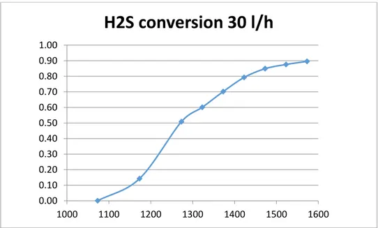
Figure 34 - conversion of H2S for 30 l/h of volume flowrate ... 54
Figure 35 – mass fraction of H2S for 30 l/h of volume flowrate ... 55
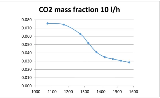
Figure 36 – conversion of CO2 for 10 l/h of volume flowrate ... 56
Figure 37 – mass fraction of CO2 for 10 l/h of volume flowrate... 56
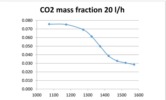
Figure 38 - conversion of CO2 for 20 l/h of volume flowrate ... 57
Figure 39 - mass fraction of CO2 for 20 l/h of volume flowrate ... 57
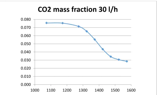
Figure 40 - conversion of CO2 for 30 l/h of volume flowrate ... 58
Figure 41 - mass fraction of CO2 for 30 l/h of volume flowrate ... 58
Figure 42 – C++ code. BzzNonLinearRegression initial data ... 61
Figure 43 - C++ code. Regression command ... 61
Figure 44 – kinetic scheme initializing, regression parameters... 62
Figure 45 – kinetic scheme initialization, writing kinetic file ... 63
Figure 46 - kinetic scheme creation ... 63
Figure 47 – DSmoke input data for regression ... 64
Figure 48 – compiling file.dat for DSmoke ... 66
Figure 49 – simulation Run file ... 67
Figure 50 – reading the results in .DTM file ... 67
Figure 51 – finding the results of the .DTM file ... 68
Figure 52 – assigning y of the model ... 69
Figure 53 – H2S comparing conversion 10 l/h ... 72
Figure 54 – H2S comparing concentration 10 l/h ... 72
Figure 55 H2S comparing conversion 20 l/h ... 73
Figure 56 - H2S comparing concentration 20 l/h ... 73
Figure 57 - H2S comparing conversion 30 l/h ... 74
Figure 58 - H2S comparing concentration 30 l/h ... 74
Figure 59 – CO2 comparing conversion 10 l/h ... 76
Figure 60 – CO2 comparing concentration 10 l/h ... 76
Figure 61 - CO2 comparing conversion 20 l/h ... 77
Figure 62 - CO2 comparing concentration 20 l/h ... 77
Figure 63 - CO2 comparing conversion 30 l/h ... 78
Figure 65 – Brooks® Instrument fluximeter used in the laboratory ... 82
Figure 66 – Brooks® Instrument set point controller ... 82
Figure 67 – Swagelok plug valve used in the laboratory ... 83
Figure 68 – reactor shape in AutoCAD ... 83
Figure 69 – tube furnace Carbolite® Gero series ... 84
Figure 70 – Dynsim™ workspace ... 86
Figure 71 – example of thermodynamic choose in Dynsim ... 87
Figure 72 – icon Palette: base equipment ... 88
Figure 73 – example of Instance tree... 90
Figure 74 – example of Simulation Status Panel ... 91
Figure 75 – example of Snapshot Panel ... 91
Figure 76 – N2 source modelling ... 92
Figure 77 – choice possibility using ‘connector’ ... 94
Figure 78 – fluximeter reproduced in Dynsim ... 94
Figure 79 – pre-reactor section in Dynsim ... 95
Figure 80 – example of one element of PFR reactor in Dynsim ... 97
Figure 81 – Feeds and products configuration of the reactor ... 98
Figure 82 – ‘Reactions’ tab in the AG2S™ process ... 98
Figure 83 – Reaction Data Set ... 99
Figure 84 – Reaction data ... 100
Figure 85 – PFR reactor in Dynsim ... 100
Figure 86 – External inputs in the utility exchanger ... 102
Figure 87 – user defined orientation of drums in Dynsim ... 103
Figure 88 – user defined orientation example ... 103
Figure 89 – complete process scheme in Dynsim ... 105
Figure 90 – trend of N2 flowrate in 30 l/h case ... 105
Figure 91 – Reactor dynamic window ... 106
Figure 92 - H2S conversion results at 10 l/h ... 107
Figure 93 - H2S conversion results at 20 l/h ... 108
Figure 94 – H2S conversion results at 30 l/h ... 108
Figure 95 - CO2 conversion results at 10 l/h ... 109
Figure 96 - CO2 conversion results at 20 l/h ... 109
Figure 98 – MOSAIC workspace ... 115
Figure 99 – notation tab structure ... 116
Figure 100 – MOSAIC different groups of symbols ... 117
Figure 101 – example of equation ... 118
Figure 102 – example of an equation system ... 120
Figure 103 – ‘Simulation’ evaluation section... 127
Figure 104 – ‘Indexing’ in ‘Simulation’ section ... 128
Figure 105 – instantiated reactor system ... 129
Figure 106 – specification window ... 129
Figure 107 – particular of notation description in ‘variable specifications’... 130
Figure 108 – import section in ‘Specifications’ window ... 130
Figure 109 – code generation ... 131
Figure 110 – massive fractions of H2S vs reactor temperature, 10 l/h ... 132
Figure 111 - massive fractions of H2S vs reactor temperature, 20 l/h ... 133
Figure 112 - massive fractions of H2S vs reactor temperature, 30 l/h ... 133
Figure 113 - massive fractions of CO2 vs reactor temperature, 10 l/h ... 134
Figure 114 - massive fractions of CO2 vs reactor temperature, 20 l/h ... 134
Figure 115 - massive fractions of CO2 vs reactor temperature, 30 l/h ... 135
Figure 116 – orthogonal collocation notation... 136
Figure 117 – orthogonal discretization equations... 136
Figure 118 – collocation matrix... 137
Figure 119 – index matching in discretization transformation ... 138
Figure 120 - state variable determination in the discretization transformation ... 138
Figure 121 – reactor system discretized ... 139
Figure 122 – dampening factor in the discretized reactor ... 139
Figure 123 – temperature results after the natural cooling section ... 144
Figure 124 – ports and streams configuration ... 155
Figure 125 – notation of the interface ... 156
Figure 126 – interface creation ... 157
Figure 127 – connector between reactor and stream ... 157
Figure 128 – connector between stream and natural cooling ... 158
Figure 129 – connector between natural cooling and stream ... 158
Figure 131 – printed natural cooling section ... 161
Figure 132 – entire process equation system ... 162
Figure 133 – edit internal streams ... 162
Figure 134 – internal streams creation: output port ... 163
Figure 135 – flowsheeting of the entire process in MOSAIC ... 164
TABLE INDEX
Table 1 – kinetic parameters results after data regression ... 70
Table 2 – Dz finite elements of the complete reactor evaluation ... 142
Table 3 – example of first trap results ... 147
Table 4 – atomic matrix for the second trap system ... 149
Table 5 – example of trap 2 results... 151
Table 6 – complete results for trap 2 and trap 3 at 10 l/h ... 152
Table 7 complete results for trap 2 and trap 3 at 20 l/h ... 153
ABSTRACT
Abstract in italiano
La Simulazione Dinamica Immersiva in 3D può rappresentare un nuovo approccio nella formazione degli operatori in ambito industriale o di laboratorio. Tramite la formazione immersiva in 3D gli operatori possono infatti sperimentare differenti scenari di lavoro, incluse simulazioni di incidenti, con il valore aggiunto della perfetta riproducibilità delle simulazioni ed in completa sicurezza. Inoltre, sarebbe possibile introdurre all’interno delle simulazioni un sistema di valutazione delle performance degli operatori, in modo da avere diretto riscontro dell’efficacia della formazione. Questo lavoro di tesi si propone di gettare le basi per la realizzazione della simulazione dinamica immersiva di un esempio reale applicativo, producendo il modello ingegneristico in 3D e la simulazione dinamica del processo sperimentale di laboratorio AG2S (Acid Gas To Syngas) ed analizzando il potenziale dell’ambiente di simulazione MOSAIC (realizzato presso l’università TU Berlin) come fulcro di gestione del processo di virtualizzazione. Il processo AG2S sperimentato presso il Politecnico di Milano si propone di produrre Syngas, gas combustile commercialmente di valore, a partire da gas acidi quali la CO2 e l’H2S, prodotti di coda
provenienti dalla desolforazione di Syngas da carbone, potenzialmente dannosi e/o tossici per l’ambiente e per l’uomo. La scelta di un esempio applicativo reale in scala di laboratorio simboleggia inoltre la volontà di realizzare il progetto al fine di consentire la formazione di operatori non solo di processi industriali, bensì anche di laboratorio.
Abstract in inglese
The 3D Immersive Dynamic Simulation can be a new approach for industrial and laboratory operators training. With an immersive 3D training the operators could experience different work scenarios, including accidents, with the added values of complete safety and perfect reproducibility of the simulations. Besides, it could be also possible to assess the operator performances during the simulation, in order to have a better evaluation of the training efficacy. This thesis work lays the basis for the 3D immersive simulation realizing of a real application, producing the 3D model and the dynamic simulation of the AG2S (Acid Gas To Syngas) lab scale process, and analyzing the potential of MOSAIC simulation environment (realized at TU Berlin University) as HUB of the virtualize process. The AG2S process wants to produce Syngas, combustible gas commercially valuable, starting from acid gases like CO2 and H2S, tail gases from the
desulphurization of coal Syngas, potentially dangerous and/or toxic for humans and environment. The choice of the lab scale case of study symbolizes even the possibility to perform the 3D immersive simulations not only for the industrial operators, but also for the laboratory operators training.
1. IMMERSIVE DYNAMIC SIMULATION:
instruments and goals
The final goal of this project is to realize an Immersive Dynamic Simulation of a chemical process. An immersive simulation of the process can be useful to reproduce the operators training in a virtual 3D environment. The potential of the immersive simulation is to reproduce an environment that gives similar ‘sensations’ of the real plant to the operators, in order to realize a training where they feel ‘immersed’ exactly in the plant.
With an immersive 3D training the operators could experience different situations as they are in the plant, but with the added values of complete safety and perfect reproducibility of the simulation. With this kind of training, the operators could be tested in all the possible scenarios of the plant, including also accidents with a proper simulator. Besides, it could be also possible to assess the operator performances during the simulation, in order to have a better evaluation of the training efficacy.
This work is focused on the creation of a first example of Immersive Dynamic Simulation. For this purpose a chemical process with a new experimental laboratory at the ‘Politecnico di Milano’ university is selected to be reproduced in the immersive 3D environment. The selected process is the AG2S (Acid Gas To Syngas), licensed by professor Flavio Manenti.
In this first chapter a brief introduction of the principal components to be used in order to realize the immersive dynamic simulation is presented.
1.1 HOW TO CREATE AN IMMERSIVE DYNAMIC
SIMULATION
An immersive dynamic simulation is the result of a very complex harmonization between different instruments:
3D reproduction of the plant. This is the starting model which contains all the equipment in their real position in plant and with the same dimensions and engineering characteristics like temperature and mechanical resistance or construction material.
Process Dynamic Simulation. The plant has to be dynamically simulated to reproduce, during the operator training simulation, its real behavior depending on the operator’s actions.
3D virtualization of the process. Thanks to specific software the 3D model and the dynamic simulation are used as inputs to ‘virtualize’ the plant. In this phase all the textures and lighting effects to the 3D are applied to produce a good immersive effect of the virtual plant.
Generalizing language software. This work also tries to generalize the input that 3D virtualization software has to receive. As regards 3D plant models, there is a worldwide usage (more than 80%) of Intergraph® Smart3D; but in dynamic simulations contest, there is not prevailing software. This is why it could be very useful putting an ‘interface’ environment between the dynamic simulation software and the virtualizer which is able to ‘generalize’ the output of the dynamic simulation to produce a standard input for the 3D virtualization of the process, whatever the dynamic simulation software used.
This master thesis work is focused on the creation of all the elements needed for the 3D virtualization of the real application chosen, the AG2S™ process, creating the 3D plant reproduction and the process dynamic simulation; besides, in the last part of the study one possible way to generalize the dynamic simulation inputs to virtualization software is presented.
The most important software used in the thesis project are listed and described in the following.
1.1.1 Intergraph® Smart3D
The 3D model of the plant is realized with Intergraph® Smart3D.
This program is released on 2014, from the consolidation of SmartPlant® 3D, SmartMarine® 3D and SmartPlant® 3D Materials Handling Edition, and it’s a design software specifically tailored for plant, offshore, shipbuilding metals, mining and bulk material handling industries. It employs an engineering approach of the 3D model: every equipment, slab, piece of architecture has not only dimension characteristic, but even other engineering proprieties, like construction material, temperature and pressure resistance.
Every piece of the plant has a collocation in the huge database provided by Smart® 3D, in which there are piping, reactors, heat exchangers, typical chemical process equipment, and all the civil components used to produce the substructure of the plant, like girders, beams, columns, electric components, and also some choices of architectural buildings.
Intergraph® Smart 3D enables also to introduce new equipment in database if they are not already present.
1.1.2 Simsci™ Dynsim
The Dynamic Simulation of this work is made with Simsci Dynsim.
Dynsim is a dynamic process simulator that enables to design and operate a process plant including the control system design and improve process yield reducing the capital investment costs. It includes a big database for chemical compounds that could be even expanded, and models for the most important chemical process utilities, like reactors, heat exchangers, valves and process controls.
With Dynsim it’s possible to simulate the dynamic behavior of the plant, from the turn on to the shut off, with a manual or an automated control system. This software is able to calculate the behavior of fluids in piping, thermodynamical equilibrium in flashes, rate of reactions in PFR, CSTR and non-ideal reactors, it can simulate also furnaces, distillation columns and other complex equipment.
1.1.3 MOSAIC
Mosaic is the program chosen to try to convert the output of whatever dynamic simulator into a standard input to the virtualization software.
Mosaic is a modeling, simulation and optimization environment. Based on a LaTeX-style entry method for algebraic and differential equations, systems can be built and used for simulations. Besides, Mosaic provides an automatic code generation for numerous simulation and optimization environment, like Matlab, Ampl, Modelica, gProms, and solvers interfaced via C++, Fortran, Python and others.
Thanks to its ability to convert languages and its open structure to model systems of equations, Mosaic could be able to receive an output from the dynamic simulator and convert it in a generalized input for the virtualization software.
The general overview of the project is illustrated; in the next chapter few considerations are reported to better explain the thesis work objective but also to introduce the future completions to this first step toward the final goal.
2. THESIS OBJECTIVES AND FUTURE STEPS
The previous chapter presents the main instruments used in this thesis work, excluding with DSmoke which will be described in the following chapters. At the beginning of the thesis project the results to achieve have been fixed; the most important results to reach were the 3D modelling of the studied process, the dynamic simulation complete of a new simplified kinetic scheme for the reactions considered, and finally a deep analysis on the MOSAIC simulation environment and the study of its potential in the Immersive Dynamic Simulation project. All these goals are reached during the long path of this thesis work, with alternation of successes and failures, unexpected problems and sudden great progress. The final result of all the efforts and gratifications of this master degree thesis is presented in the next chapters. The chosen order of description reflects the effective chronology in which the different arguments have been faced: the first section of the thesis regards the 3D model of the process, in the second section all the kinetic regression and dynamic simulation problems are addressed, and in the last section the study of MOSAIC environment is reported using the AG2S™ process as an example to show the most important characteristics of this program. In conclusion, the thread which connects all arguments and instruments used in this thesis work, very different each other, is exactly the
AG2S™ process, which acts as useful example to show all the most important
characteristics of the software used, and provides the first real challenge for the Immersive Dynamic Simulation project, which could embrace not only the industrial chemical processes, but also the lab world, in a completely new perspective of which this thesis work is the perfect symbol. In fact, the usage of industrial software i.e. Intergraph® Smart 3D or Simsci Dynsim to perform a laboratory scale 3D model and dynamic simulation has been a big challenge, but the potential of Immersive Dynamic Simulation in the lab scale is as big as in the industrial scale, because the possibility to train the operators before going the laboratory is a real need, which in the university world is settle with the usage of global safety trainings; lots of times the training for the specific activity to do in the laboratory is very lacking, and it needs more consideration. Using the Immersive Dynamic Simulation for the laboratory activities means to ensure the safety and the right working of the operators, training them for their specific mansions and certifying the learning level before allowing the access in the work place, at the cost of producing the engineer 3D model and the dynamic simulation of the laboratory. The same concept can be extended to the
industrial work, where even more attention is taken on the safety and performances of workers, and where industrial simulators and 3D models are still available to be used for the Immersive Dynamic Simulation, so the problem is focused mostly on the standardization of the simulator output and on the connection with the virtualizer. This thesis work has the presumption to guarantee the prerequisites for finding the right solutions in both the situations, with a double focus on the industrial scale and the lab scale. The perfect representation of the double valence of this project is the usage of industrial engineer software like Intergraph® Smart 3D and Simsci Dynsim to reproduce a lab scale process like the AG2S™ process. In this way it’s possible to verify the difficulties and opportunities in the 3D immersive dynamic simulation in both the scenarios, as in the industrial case the need to standardize the output of dynamic simulation trying to use MOSAIC environment, but also the lab scale problems like the actual 3D model restrictions in terms of dimensions and availability of lab scale process components.
Despite the large number of topics addressed in this thesis work, the Immersive Dynamic Simulation project has to face lots of other problems; the first problem is the visual rendering of the 3D model in order to create a realistic texturing and lighting of the components. This operation can be made only after the 3D model creation, and probably inside the virtualizer in order to enable a dynamic changing of lighting and shadows depending on the operator position; at this point this kind of problems are not considered, but in the development of the project this will be a crucial aspect to guarantee the operator immersion in the simulation space, and people with other skills are needed to reach a good result. The 3D environment with the Smart3D structure has to be rendered in order to obtain realistic coloring, shading and reflection effects of the equipment; texturing must be accurate and reflect the real conditions of the components, including fouling and rusting, because the operator must perceive the immersive environment like the real one, with all its imperfections. This is necessary because the worker is trained to specific operations to be done in the workplace, and must associate the actions done during the immersive training as the real acts to do subsequently in the real plant, and the effectiveness of that association is strongly dependent on the correspondence of not only shape, dimensions and position of equipment, but also their textures.
Another problem to be faced hereafter is the linking between all the different software necessary to perform the immersive simulation. The connection between the 3D model and
the dynamic simulation must be the task of the virtualizer, but how to send the information from this software and receive and manage them into the virtualizer is another important future object of study. The integration with MOSAIC can be a solution to standardize the output of the dynamic simulation, but even in this case the way to send and receive information must be deepen. In the MOSAIC section of this thesis work the potential but also the limits of this simulation environment will be presented, and it’s possible to anticipate already in this introductory chapter that the biggest problem at now it’s the real-time communication in MOSAIC, which is not expected in the current version of the software. Even without the mediation of MOSAIC, the connecting process between different software preserves its intrinsic difficulty, and people with specific informatics skills are required to get it possible.
The greatest charm and complication of the 3D Dynamic Immersive Simulation project is the necessity to really high and various competences, which go from the engineering world with dynamic simulation, 3D model and language flexibility knowledge, to 3D rendering and texturing, informatic design and data exchange complexity which are designer, architectural and informatic competences.
The current state of the project is focused on the engineering contributes, which are the preliminary necessary steps to provide all the required data to start including the other competences. In this case the engineering work is the fundamental substrate over which building the artifices to reach the final goal. But, even within only the engineering contribute of the project, the competences required are really various; the 3D model production, a completely new skill to be learned, the dynamic simulation of the process flanked to the generation of a regression code using a mathematic library, and finally the discovery of a totally new simulation environment, with specific language and model construction rules, are an incredible challenge to be performed by a single person, but also an amazing personal enrichment. The possibility to see the entire process with different points of view has been a beautiful opportunity which enables to further understand the complexity and beauty of the engineering world. Even if the huge amount of the new competences to be learned seemed prohibitive, each difficulty has been overcome step by step, and the thesis work results are very satisfactory.
These considerations conclude the introduction section of this work; in the next chapters the whole thesis work is presented and depth, from the beginning to the final results, starting from the 3D modeling of the process.
3. 3D MODELING: INTERGRAPH® SMART 3D
As written in the introduction, Intergraph® Smart 3D is the software chosen to produce the 3D modeling of the laboratory. The choice was made because of the ‘engineering approach’ of the program, with the possibility to insert not only geometric proprieties of the process components, but even lots of different characteristics which are representative of the equipment and which can be useful in the virtualizing phase. In the next chapter the principal components of the Smart 3D workspace are presented.
3.1 SMART 3D WORKSPACE
The workspace represents the model data. Smart 3D operates through ‘tasks’, which can be selected in the home screen.
Different ‘tasks’ operates with different parts of the plant. The main tasks used in this work are: - grid - piping - equipment - structural system
3.1.1 Task grid
During the construction of the 3D model, there is the need of a reference system; this could be global (which follows original coordinate system) or relative (following a coordinate system determinate by the user).
For this scope the grid task is useful to create reference planes in the workspace. In this way it’s easier to place the objects in the right position, using a local reference instead of the global which can be uncomfortable in lots of cases.
Figure 2 – radial grid
In this work grids are used to define the three planes of the chemical laboratory, i.e. the main plane with the fume hood base, and the two planes which support fluximeters and micro gc.
3.1.2 PinPoint
Another very important instrument of Smart 3D to change the local coordinate system is PinPoint command.
This command enables to select every point of the workspace defining it as the origin of new relative coordinate system. As Smart 3D recognizes crossing point between objects, axes of the structures and middle point of the planes, it’s possible to choose one of these crucial points as the PinPoint. In this way it’s possible to create complex equipment or architecture with beams in an easy way.
3.1.3 Structural System task
The structural system task is dedicated to the creation of slabs, walls, columns, beams, and all the others objects with structural functions.
Smart 3D database contains many types of construction components, differentiating by section shape, dimensions and material proprieties with European and ASTM standards.
Figure 5 - structural system editor bar
With structural system task, it’s possible to create all the civil components of the plant. It is also possible to connect or split axis, to insert stairs and railings, in order to reproduce the real supporting system.
3.1.4 Equipment task
The equipment task is able to reproduce the chemical process components of the plant; in particular it models reactors, heat exchangers, pumps and compressors, distillation columns, tanks and vessels, but also safety showers and electrical or architectural components.
Figure 7 – example of vertical vessel equipment
It’s possible to use defined equipment ( symbol), which is present in database; to help to choose the right designed equipment from the many possibilities available in the system database, it’s also provided a preview that contains a schematic illustration of the equipment reporting its most important components with an identifying symbol.
Figure 8 – example of designed equipment with preview
It’s often possible to modify dimensions of the designed equipment to create it like the real one, but this type of modeling has some restriction. In fact every nozzle dimension, length
of a piece of equipment or diameter of the component, has to respect the limiting minimum and maximum programmed values.
For these reasons, in the equipment task it’s also provided a ‘place not designed equipment’ section ( symbol). Even in this case, the choice of the equipment in the database is mandatory, but it’s only a way of the system to assign the non-designed component in a subgroup, for example in this thesis work we chose ‘complex horizontal vessel’ as subgroup of the laboratory reactor.
After the choice of the non-designed equipment subgroup, it’s possible to start modeling the equipment. To produce a highly customized solid different shapes are available ( symbol); they can be added or subtracted in a global solid ( symbol) which could represent the entire equipment or only a part of it. Also for the available shapes there is a special catalogue in which is present their preview.
Figure 9 – shapes catalog with preview
Differently from the designed equipment, shapes are completely modifiable in all their dimensions without any limiting value (but they must be real dimensions, negative numbers are not allowed). For some of the shapes present in the database, it’s also possible to modify angles between sides to produce particular piece of equipment; during the laboratory modeling this special characteristic is used in particular pieces of the reactor.
Shape can be added ( symbol) or subtracted ( symbol) using the ‘place a solid’ tool, which is the way of the system to recognize as a unique solid the combination of single shapes. This type of system structure leads to the fact that shapes can have only dimension
characteristic, while material proprieties, T and P resistance and all the others parameters are associated to the solid. This could be a problem when equipment is composed by pieces with different proprieties, like for example the tube furnace of this thesis work. In that case, it’s necessary to produce different solids for the metallic base of the furnace and the refractory tube.
Thus, producing equipment with ‘place a solid’ tool enables to model a totally customized equipment, but it requires obviously much time in respect to ‘place a designed equipment tool’.
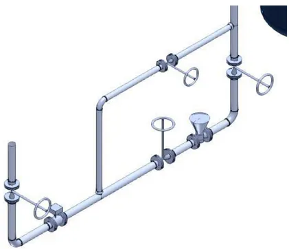
3.1.5 Piping task
The piping task enables to create in the 3D model all the components concerning pipelines, i.e. not only piping but even valves, flanges, taps, nozzles and special components like fluximeters.
In the following the actions that can be performed in the Piping environment are presented: Create and route a pipe run: it’s possible to create pipe run, extend an existing one, and route a pipe run to or from nozzles and equipment inlets or outlets;
Insert splits: it’s possible to insert splits into the pipeline. It could be useful to divide a pipe run into sections by placing a set of flanges, a union component, or to move one block of the pipeline without modifying the other parts.
Insert pipe components and custom instruments or specialty items: it’s possible to insert pipe components to create sophisticated pipe layouts that divide, branch and convey fluids between equipment. This is the case of fluximeters used in the laboratory modelling. Add taps on pipe components: it’s possible to add taps to standard components such as caps, instruments, orifice flanges, and valves.
Besides pipelines can be characterized by lots of proprieties:
- Design and Operating Maximum and Minimum Temperature - Design and Operating Maximum and Minimum Pressure
- Surface Treatment and Coating: interior and exterior surface treatment, cleaning requirement, auxiliary treatment requirement, interior and exterior coating area and type, coating color
- Insulation and tracing: insulation purpose, material, thickness, temperature, tracing requirement, type
- Responsibility: party responsible for cleaning, design, fabrication, installation, painting, requisition, supply, delivering, testing on
Figure 10 – complex piping example
3.2 SMART 3D MODELING OF THE LABORATORY
In this master thesis project Smart 3D is used to model the AG2S™ laboratory at the ‘Politecnico di Milano’ University.
The laboratory is an experimental unit for the AG2S™ process, which wants to produce syngas (CO and H2) from tail gases containing H2S and CO2, undesirable products. A
3.2.1 Preliminary studies
The main components of the laboratory to be 3D modelled are:
Structural elements:
- all the support planes, specifically the fume hood base and the fluximeters and microgc supports;
- the wall behind the fume hood;
Equipment:
- base of the fluximeters; - tubular furnace; - glass reactor; - microgc; - metallic trap; - flasks trap; Piping:
- piping from the inlet of the fume hood to the fluximeter; - piping from the fluximeter to the reactor;
- piping from the reactor to traps and to microgc; - piping between traps;
- outlet piping which end in the fume hood top.
The 3D model is realized in collaboration with Intergraph® Company, the provider of Smart 3D software. The company organizes three tutoring sessions to help the laboratory 3D modeling. A preventively 2D CAD of the little plant is requested by Intergraph to provide specific help with the laboratory modelling. In the following the 2D CAD work realized for Intergraph is reported.
Figure 11 – plant of the laboratory realized in Autocad®
Figure 12 – frontal prospectus of the laboratory
It’s possible to see all the components listed previously. In particular the most complex pieces of equipment are reported with different colors to facilitate the comprehension of the CAD: fluximeters are realized in violet, the furnace in red, the first trap in orange and the reactor in light blue. All the pipelines are realized in dark blue while other components of the project are grey. It’s also possible to see all the quotes of the laboratory components, which are reported in [mm].
After the 2D CAD creation, the 3D modelling part can begin with a specific tutorial made by Intergraph.
3.2.2 Structural system realization
The first part of the 3D realization is dedicated to the structural scheme of the laboratory. The use of grids is useful to create three planes over which construct the slabs that represents the structural elements.
To create the elements, the ‘Slab’ command ( symbol) is used, which enables to create horizontal supports with variable thickness and material proprieties. To position the slabs the grids previously created are used.
Also the wall behind the fume hood is created using ‘Structural System’ task. After the creation of grids and slabs, it’s possible to choose a reference plane to create a wall of which position is linked to it using the ‘Wall’ command ( symbol). This is perfect to produce the laboratory wall, because it must be placed in correspondence of the previously created slab. In the general overview section (3.2.5) it’s better explained the way to reproduce walls in Intergraph® Smart 3D.
3.2.3 Equipment realization
After the structural system, equipment components are created. This is the main part of the work, because unfortunately Smart 3D database doesn’t contain any equipment of the laboratory. In fact, Intergraph® Smart 3D is programmed for the creation of industrial plant 3D models, while in this work is used for a laboratory scale 3D modeling. In equipment section the designed components have a larger order of magnitude of ‘Minimum and Maximum Values’ to be assigned in respect to the laboratory real dimension; besides, the reactor section is highly customized to respect the experimental requirements. The only way to model equipment section too little and customized to be created with ‘designed equipment’ tool is to produce it using shapes and solids.
For every different diameter section of the reactor, it’s necessary to create a couple of conical or cylindrical shape: the first shape represent the real section of the reactor, the second one has to be subtracted to create the effective void, otherwise the reactor would be like a full glass component without any correspondence to reality. Another difficult of the equipment, and in particular reactor, modelling, comes from its peculiar shape. The outlet part of the reactor is the most difficult to reproduce, because it contains very complex
conical sections with rotation angles, the worst shape to reproduce in Smart 3D. It can be possible to notice them in the figures below:
Figure 13 – particular of the reactor outlet in Autocad®
Figure 14- particular of the reactor outlet in Smart3D
In both the figures the outlet of the reactor is represented, including the junctions to the two pipelines exiting it: at the left, the pipeline that goes to the traps, on top the pipeline to the microgc analysis.
In the following figures the inlet part of reactor reproduced in AutoCAD and Intergraph® Smart 3D is reported. It’s possible to observe the same modelling difficulties of the outlet part, with lots of different diameters sized components which have to intersect themselves without interpenetration of corps. These specific fittings for the reactor is clearer in the AutoCAD™ representation, but they are perfectly reported even in the 3D model; in the virtualization software, it will be possible to ‘clothe’ the Smart 3D project with specific textures which can reproduce the reactor glass transparency. In this way, also the covered components in the reactor 3D model will be observable like in the AutoCAD™ project.
Figure 15 – particular of the reactor inlet in AutoCad™
Before passing to the trap equipment, it can be interesting to observe the model scheme database through the ‘workspace explorer’ tab. In particular in the figure below the model scheme database of the reactor is reported.
Figure 17 – workspace explorer: reactor
Figure 18 - workspace explorer: reactor_2
In these figures it’s easily recognizable the schematic structure of Smart 3D system. The first object to define is the ‘not designed equipment’, which in this case is: Reattore. Then it’s possible to create a solid, Reattore-Shape-0001, associated to the designed equipment. In this case it’s necessary only one solid because all the reactor components have the same proprieties. After the solid definition, shapes ( ) can be created. Every
shape can be added or subtracted from the solid to eventually create the reactor model; the plus or minus symbol near every shape describes the shape function within the solid. It’s interesting to observe that are necessary about 60 shapes only for the reactor model, a huge number derived from the highly customized form to be reproduced.
After the reactor realization other equipment has to be modelled. In particular, the most complex pieces to be created are the traps, which in the real laboratory are used to remove sulfur and H2S residuals from the product flow. The first trap is a metallic cylindrical
component with a tube section for the product flow, and a shell section for the cooling water that must lower the temperature of the process outlet. The reproduction of the first trap is illustrated in the figures below:
Figure 20 – metallic trap model with Smart 3D
It’s possible to distinguish, in particular in 3D model of the trap, the tube and shell sections realized with the adding and subtractions of different shapes to compose the concave part filled with water and the internal part for the process flow.
The other traps used in laboratory are simple flasks filled with a solution of NaOH and NaOCl used to separate H2S by the product. The biggest one, which receives the outlet
flow of the metallic trap, is reported in the following page. The other trap has the same construction modality but with different dimensions.
Figure 21 – flask trap model with AutoCad™
Figure 22 – flask trap model with Smart 3D
The equipment section is defined. There are other equipment components like the junctions of every piping, some little part of fluximeters and microgc, but they are created using few shapes and they can be observed in the final general view of the laboratory, without a
3.2.4 Piping realization
Piping is the final section to be produced. All the other components must be created and placed in their real positions; in this way it’s possible to create a realistic path of pipelines which should correspond to the real one.
Intergraph® Smart 3D, as seen before, provides dedicate piping section. It’s possible to produce pipelines with complex paths, choosing the right angle of curvature of tubes. The system can calculate if the imposed angle is feasible for the chosen pipeline, in particular in respect to its physical proprieties reported in database. If an unfeasible angle of curvature is chosen for the tube, Smart 3D suggests a welded section to reproduce the same trajectory of the original intent, but using three different tube parts in order to preserve the real feasibility of the 3D model.
Piping section is also used in this work to produce fluximeters, which are managed by the system as ‘special equipment’ linked to the pipelines. The link between piping and fluximeters is evident during the creation of these components. In fact, Smart 3D enables the creation of ‘special equipment’ only with the presence of a pipeline that can be connected to the fluximeter. It’s impossible to model a fluximeter without the creation of its referring pipeline.
In the laboratory 3D model, ‘Piping’ task is used to produce fluximeters that must control the process flowrate to the reactor, and all the pipelines associated to the fume hood, from the inlet of the fluximeters to the outlet to the top of the fume hood. In the case of AutoCAD™ project, it’s not necessary to model pipelines with their specific thickness, because that is only a preliminary work to decide together with Intergraph ® Company the best way to model the laboratory. Obviously it’s very important to model in AutoCAD all the equipment with their real dimensions and in their real positions.
In the figure below the fluximeters section and inlet reactor pipeline are reported. As previously mentioned, only Smart 3D pictures are illustrated.
Figure 23 – fluximeters section and inlet of the reactor on Smart 3D
It’s possible to observe that, in this 3D project, different colors belong to different system sections. In fact, the red beams construction is produced with ‘Structural System Task’, while the grey pipelines and fluximeters are created with ‘Piping Task’; at last, the reactor, furnace, pipeline fittings, shut-off valves and also the support of the fluximeters are made by ‘Equipment Task’, so they’re represented in blue color. The only exceptions are the structural components like walls and slabs, which system produces in standard grey color.
It’s interesting to report a section of the workspace explorer of pipelines:
Figure 24 – workspace explorer: piping
In this way it’s possible to observe the system characterization of piping: in the main ‘Piping Flussimetri’, all the pipelines that go from and to fluximeters are included. Every pipeline is then decomposed to the single pipes that form the entire object. In this way Smart 3D is able to produce automatically pipelines with specific curvatures, assembling single pipes which compose the final result.
It’s also interesting to observe that, as said before, fluximeters are considered as a special piping object. In the figure above the three fluximeters ‘pipelines’ are reported: they consist of the special object ( symbol), and the two pipes which are connected with the fluximeter.
3.2.5 3D model complete
With the piping realization the 3D model of the laboratory, as regards the fume hood, is complete. The environment around the fume hood, which includes the laboratory room, the external structure of the fume hood and all the elements linked to them, will be created in collaboration with Architectural Department of Politecnico di Milano using laser scanning technique to produce a points cloud. This cloud can be imported in Intergraph® Smart 3D to produce a substructure of the environment which enables to easily reproduce it in the workspace.
In this section it’s possible to appreciate the overview of the laboratory 3D model created on Intergraph Smart 3D.
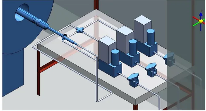
Figure 25 – front panoramic overview of 3D laboratory
In this front overview are visible the most important components of the laboratory. From the left to the right there is the microgc, under it there are the three traps, then the reactor, furnace and finally the fluximeters over their structural support. It’ also observable the ending pipeline, which starts from the last trap and go to the top of the fume hood, where the outlet flows can be aspirated.
Figure 26 – Top panoramic overview of the laboratory on Smart 3D
In the top overview of the 3D model the positioning of the laboratory components is better observable. It’s also possible to recognize the three different pipelines of H2S, CO2 and N2,
entering the fume hood and going to the fluximeters. In the panoramic overview is also highlighted the complex placing of all the equipment, due to the necessity to use an already available fume hood in the laboratory room chosen for the experimentation; in fact in this picture it seems that furnace interpenetrates the fluximeters structure, but it’s possible to see in the front overview and even in the following pictures that furnace is above the fluximeters table without interpenetration problems. Because of the fact that laboratory is not completely assembled during the AutoCAD and 3D production, one of the crucial aspect of this work is to discuss and realize the positioning of all the laboratory components. This is the final result of the preliminary study, which satisfies space optimization and safety criteria.
Figure 27 – right panoramic overview of the laboratory on Smart 3D
In the right panoramic overview is more evident the three-dimensionality of the model. Besides, it’s possible to better observe the wall behind the fume hood: because of the Intergraph® Smart 3D options for wall structures, it’s allowed to place a wall only under, above or in the middle of the reference plane chosen. In this case the reference plane is the base of the laboratory, and the wall has different heights in the below and above sections in respect to the table. In fact, as seen in the picture, the above section of the wall is taller than the below section. For this reason, to produce this part of structural system, a unique wall component isn’t sufficient, because none of the three alternatives to place the structural part is valid: choosing under or above the plane configuration, the entire wall would be placed in a wrong way, but also with the middle plane configuration, real dimensions would not be respected. The only way to reproduce faithfully the wall on Smart 3D is creating two wall parts, the first placed below the reference plane, and the second above it. Observing with attention the figure 25 is recognizable the particular structure of the wall.
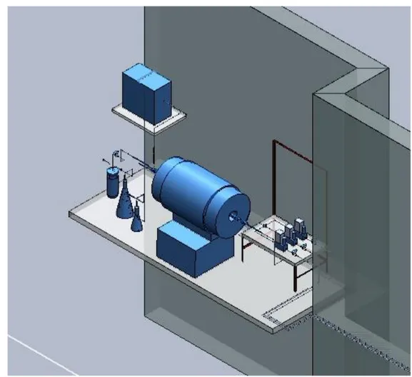
Figure 28 – left panoramic overview of the laboratory on Mosaic
At the end, the left panoramic overview is presented.
It results very similar to the previous one, but it’s better to appreciate the exiting section of the reactor and the three traps linked with piping.
4. BEFORE PROCESS SIMULATION: REACTION
KINETIC
4.1 AG2S PROCESS DESCRIPTION
At this point, only the laboratory structure is presented because of its importance in the 3D modelling. Before approaching the dynamic simulation, it’s instead necessary to deepen the description of the AG2S™ process, and in particular to the reactions involved, in order to find good kinetic data.
Having good kinetic data of the reactions is a crucial point to obtain good process simulation. Unlike the thermodynamical data, which are available with good reliability for the majority of the components, kinetic data for specific reaction are really difficult to find. The reason is that no global laws to theoretically find them are known, so experimental data regression is needed. In the next paragraph description of the reactions involved, and the way used in this project to find kinetic data are presented. This preliminary work occupied a good part of the whole project, due to the difficulty to obtain satisfying results.
4.1.1 Goal of the process
The AG2S process is an innovative system to threat carbon desulfurization tail gases. Collaboration between SOTACARBO and POLIMI (Politecnico di Milano) is started to study the oxi-reduction reaction between H2S and CO2 to produce syngas composed
mainly by CO, H2 and steam. The reaction is done at very high temperature in gas phase,
and has the very interesting capacity of producing syngas, a valuable product, from H2S
and CO2, which are respectively toxic and dangerous substances. This technology could be
very useful in gasification plants where is still present a capture line of the acid gases, and so the AG2S process could be applied to reduce the pollutants emission and at the same time increase the syngas production.
4.1.2 Reaction description
Tail gases coming from desulfurization solvent regeneration consist of H2S, the main
component, CO2, CO, COS and other organosulfur compounds. The AG2S process wants
to convert these components into syngas, thanks to the oxi-reduction reaction below:
2𝐻2𝑆 + 𝐶𝑂2= 𝐻2+ 𝐶𝑂 + 𝑆2+ 𝐻2𝑂
The reaction is then able to neutralize the H2S present in the tail gases, as other conversion
process currently used, but has the advantage to valorize the hydrogen potential of the molecule converting it into H2. Besides, another crucial point is the oxidizing compound
chosen: in this reaction CO2, another dangerous acid gas, is used instead of the common air
or oxygen technology.
The theoretical results of this process show a great potential for lots of applications, with very good yields at high temperature. Obviously, before starting an industrial application of a new technology, it’s necessary to have experimental validation of the theoretical results; only after very good experimental data collection it’s possible to begin the scaling up of the process until becoming industrial application. The laboratory is built for this reason, to validate the theoretical results and proceed to the scaling up of the process.
4.2 THEORETICAL RESULTS: DSMOKE
4.2.1 How to find kinetic data
In the introduction of this chapter the difficulty to find kinetic data is presented: there aren’t theoretical laws to find reaction velocities without experimental support, and it follows that only two ways are possible to obtain kinetic data: organizing an experimental laboratory to find them, or using the available literature.
Obviously, getting data from literature is extremely cheaper and faster than organizing an experimental session; otherwise, often literature is lacking of data, because the reaction kinetic is related to the components involved and the reaction conditions, which are not only temperature, pressure and inlet flowrates and compositions, but also the presence of
catalysts and their composition. In this huge amount of possibilities, it’s really hard to find a relating process in literature of which use the kinetic data. This is valid expecially in the present case, where a new process is studied.
But, even in the case of experimental choice, a preliminary kinetic study is needed to prepare the pilot laboratory. It’s easy to understand that the experimental studies would need a series of equipment, at first the reactor, which has to be designed in all their dimensions to, in case, commission their construction or use those still available. However, focusing on the reactor, and expecially in a PFR (plug flow reactor) used in this project, the length needed to complete the desired reaction in the specific range of conditions chosen is extremely dependent on the rate of reactions involved, in other words, on the reactions kinetic. It’s so evident that to start a pilot work to find good kinetic data of the studied reactions, preliminary theoretical study of the reaction environment is necessary. In particular, good preliminary kinetic data are needed to have a good design of the laboratory which will be responsible for validating them with experimental results. Besides, having good preliminary reaction rates is very useful to study different possible new processes without the high cost of the experimental sessions, to discard the worst options and deepen the best ones. This is the case of AG2S™ process, studied only theoretically and now ready to an experimental validation of the results.
But, as written before, the reaction process is new, so there aren’t available data in literature, and the kinetic is no obtainable using a theoretical law like in thermodynamic. So how is it possible to obtain good preliminary reaction rates for the process studied? This is the role of DSmoke.
4.2.2 DSmoke introduction
DSmoke program is the software used to get the theoretical results of the AG2S™ process. Developed at the Politecnico di Milano, it allows the simulation of a sequence of different reactors eventually coupled with mixers or splitters. The program accepts only sequential schemes of reactors, i.e. in series or in parallel, but no recycle streams are allowed.
The structure of DSmoke is presented in the figure below:
Figure 29 – DSmoke structure
The first step required by DSmoke is to provide as input data the kinetic scheme and the thermodynamic data of the system. In this way the internal DSmoke interpreter can generate the kinetic model used in the simulation program. At this point, the user has to specify the operating conditions of the process to proceed to the simulation. DSmoke is now ready to calculate the output values of the process.
Several parts of this package are directly taken from the experience developed in the pyrolysis and combustion modeling at Politecnico di Milano.
4.2.3 DSmoke general features of the kinetic model
As seen before, to provide the kinetic model necessary to the simulation, DSmoke requires thermodynamic data and the kinetic scheme. As regards the first requirement, the program has been developed to work with thermodynamic data in the form used in the NASA chemical equilibrium code: seven polynomial coefficients for each different temperature range to fit specific heat, enthalpy and entropy. Temperature ranges are two, low temperature (<1500K), and high temperature (>1500K).
The thermodynamic characterization of the system follows the expressions below: 𝑐𝑝 𝑅 = 𝑎1+ 𝑎2𝑇 + 𝑎3𝑇 2+ 𝑎 4𝑇3+ 𝑎5𝑇4 𝐻0 𝑅𝑇 = 𝑎1+ 𝑎2 2 𝑇 + 𝑎3 3 𝑇 2+𝑎4 4 𝑇 3+𝑎5 5 𝑇 4+𝑎6 𝑇 𝑆0 𝑅 = 𝑎1𝑙𝑛𝑇 + 𝑎2𝑇 + 𝑎3 2 𝑇 2+𝑎4 3 𝑇 3+𝑎5 4 𝑇 4+ 𝑎 7
Therefore, for each species 14 coefficients must be introduced. Coefficients 1 to 7 refer to the upper temperature interval, while coefficients 8 to 14 are for the lower temperature interval.
In DSmoke program the thermodynamic data are already available for most of the chemical engineer interesting species, and in particular for the AG2S™ process. These data are taken from two different sources, the ‘Chemkin’ (Kee et al., 1994a, 1994b)
‘thermodynamic Data Base and the Benson’s group additivity estimation method’ (Benson,
1976).
As for the thermodynamic data, DSmoke requires default structure of chemical reaction rate expressions. The forward rate constants are expressed in the following Arrhenius temperature dependence:
𝑘𝑓,𝑗 = 𝐴𝑓,𝑗 𝑇𝑛𝑓,𝑗 exp (−𝐸𝑎𝑐𝑡𝑓,𝑗
𝑅𝑇 )
Where Af,j is the pre-exponential factor, nf,j is the temperature exponent and Eactf,j is the
activation energy of the forward kinetic constant. These data must be specified directly in the kinetic input file.
The reverse rate constants are related to the forward rate constants through the equilibrium constants. They are calculated by the DSmoke interpreter using the kinetic input and the thermodynamical data without the need to specify them in the required files.
𝑘𝑟,𝑗 = 𝑘𝑓,𝑗/𝐾𝑒𝑞,𝑗
This equation guarantees the thermodynamic consistency of the system at the equilibrium condition, where the global reaction rates must be zero.
The equilibrium constant (Keq,j) is obtained from the thermodynamical proprieties of the
components using the following expression:
𝐾𝑒𝑞,𝑗 = 𝑒𝑥𝑝(∆𝑆𝑗
0
𝑅 − ∆𝐻𝑗0
𝑅𝑇 )
In DSmoke there is also the possibility to introduce third body and fall-off reactions.
With the thermodynamic input and the chosen kinetic, DSmoke generates the kinetic model thanks to the interpreter; in this way all the reactions will have the forward and reverse kinetic constants, ready to be simulated in the specific operating conditions chosen in the following step.
In the AG2S™ process hundreds of elementary reactions are reported in the kinetic input, to reproduce the kinetic model of the system. As written before, there is no possibility to theoretically forecast the kinetic data of the reactions; all the reactions data inserted in the kinetic input of the preliminary simulation of the process are present in the DSmoke database. This huge database, taken mainly from the experience developed in pyrolysis and combustion, contains lots of elementary steps kinetic data. The global reaction of the
AG2S™ process is then divided in all the elementary steps which lead to the final products,
considering also the alternative ways that all the compounds and radical species present in the reactive system could get. In this way the kinetic input can be produced using backdata of different reactions previously studied, choosing all the elementary reactions which could occur in the actual reaction system. This work mode offers also the possibility to increase the accuracy of the model subsequently including other elementary reactions not considered in the first time, without changing the other data. In lots of applications the results of this method are consistent to experimental data with high accuracy; however, the huge number of reactions considered during the simulation can be even a negative aspect where a fast response of the simulator is needed. This is the case of the immersive simulation, where a real-time dynamic simulation is necessary to provide a good experience to the user. In the Dynsim simulation realized for the AG2S™ laboratory, it can’t be possible to introduce all the reactions considered in the DSmoke simulation. This leads to the necessity of a new simplified kinetic scheme production, which will be discussed in the next chapter.