Dendroclimatic analysis in the Adamello-Presanella Group (Central Italian Alps)

(1)

Università degli Studi di Pisa

Dipartimento di Scienze della Terra

Scuola di Dottorato di Ricerca in Scienze di Base Galileo Galilei

Programma di Scienze della Terra

XXIII Ciclo 2008 – 2010

Dissertazione Finale

Anna Coppola

Dendroclimatic analysis in the Adamello-Presanella Group

(Central Italian Alps)

Tutore:

prof. Carlo Baroni

Co-tutore: dott. Giovanni Leonelli

Referees: prof.M. Pelfini

prof. A. Carton

Direttore della Scuola

prof. Fabrizio Broglia

Presidente del Programma

(2)

Abstract

Inter annual or inter decadal climate reconstructions in the subarctic region and in high-mountain environments suffer from the absence of suitable long instrumental climate records. Annual tree-rings, along with other annually resolved natural archives, are widely used as proxies in high resolution paleoclimatology.

A temperature signal-loss has been reported in tree-rings width and density records from several temperature-limited environments since the mid-20th century, revealing a decreasing attitude of tree-ring parameters in tracking increasing instrumental temperatures.

In this study we carried out a dendroclimatic analysis on a data set of five European larch ring-width chronologies in the Adamello-Presanella Group, in the Italian Central Alps. We intended to evaluate the dendroclimatic potential of the high-elevation conifer vegetation to be used as a climate proxy, assessing the stability over time of the climate/tree-ring growth relationship.

The dendroclimatic analysis was performed by means of correlation function and response function analysis, which allowed identifying climate parameters mainly involved in rings growth. For capturing the dynamical variability of climate signal in the five tree-ring width chronologies, and to verify the stability over time of tree-tree-rings/climate relationship, moving correlation function and moving response function analysis have been used. Moreover, to test the efficiency of the tree-rings dataset for climate reconstruction purposes, we conducted a reconstruction of JJ temperature for the 1596-2004 time period.

The analysis of climate/tree ring growth relationships, producing results that are consistent with the more recent dendroclimatic studies in the Alpine Region, confirmed the presence of a common climatic signal for conifers living at the timberline ecotone.

From the monthly climatic analysis a strong positive influence of early summer (JJ) temperatures on the tree growth emerged, with June mean temperature showing the highest positive correlation. Influence of mean monthly precipitation revealed to be quite irrelevant, although we found that the five chronologies are significantly negatively correlated to June mean precipitation.

European larch confirms in this study to be a highly climate-sensitive species, with summer temperature representing the main limitig factor at the treeline. Nevertheless, a temporal instability in growth/climate response is noticeable, that means a general decreasing trend in tree-rings climate sensitivity.

(5)

Non-stationary relationships with climatic parameters may cause some concerns in tree-ring based reconstructions, which usually presume a stable response of tree-rings to climate change. The reconstruction of 1595-2004 JJ mean temperatures we performed is statistically valuable, but shows higher proficiency in describing high frequency than low frequency early mean summer temperature changes.

Overall, a decreasing skill of European larch at the treeline in the Adamello-Presanella Group in tracking increasing instrumental temperatures appears. We also found that extremely warm conditions, such as the heat wave of summer 2003, do not produce a linear response on larch tree-ring growth. Moreover, from the moving correlation analysis emerged a probable effect of a growing season lengthening on larch tree-ring growth.

(6)

1 Introduction

Human society and all the biotic and abiotic systems are strictly linked each other and their relationships are influenced by natural environment conditions. Such conditions vary continuously over time and climate plays an evident strategic role in controlling their complex driving mechanisms.

It has been widely demonstrated that in recent times climate is rapidly changing, and that it has been changing in the past (Bradley & Jones, 1992; Bradley et al. 2003; Houghton et al 1990, 2001). For these reasons a more and more large interest has been addressed by the scientific community to investigate past natural climate variability.

Detailed reconstructions of past climate and past climate variability are important tasks both in natural and human sciences. Paleoclimatic researches provide strategic bases of knowledge from which estimate future climate scenarios, their geographical extent and frequency.

Inter annual or inter decadal climate reconstructions in the subarctic region and in high-mountain environments suffer from the lack of long instrumental climate records, often caused by the existence of a few proficient meteorological stations. It appears then clear how valuable could be the presence of natural archives such as annual tree-rings that, along with other annually resolved climate proxies, are often able to provide centennial to millennial climate-sensitive chronologies. Actually climatologists‘ interest has been recently widely turned to Dendrochronology and to the various possible applications of this Science in past climate reconstructions. The relationship of Dendrochronology with the broader field of Climatology has been then consolidated and tree-ring based reconstructions of climate are at present extensively cited in all the intergovernmental climate reports (IPCC 2001, 2007).

It is widely known that tree-rings have characteristics that make them excellent sources of paleoclimatic information. For their intrinsic structure and natural physiology, they actually operate as proxies of past climate variability: it is possible to date tree-rings at their precise calendar year with a very high degree of confidence, and it has been widely accepted a linear effective correlation between tree rings from extreme environments and climate variables (Fritts, 1976, Fritts et al. 1991; Hughes et al. 1982). Moreover, tree-ring variability often presents a common signal at a large (regional) scale and, year by year, thanks to the progressive increase in the number of accessible chronologies in databases, a larger network of tree-rings data is becoming effectively available worldwide.

(7)

Since the earlier Fritts‘ studies, and especially in recent decades, a rapid improvement of dendroclimatic methodologies and applications has been developed (Hughes et al., 1982; Schweingruber, 1988, 1996; Cook and Kairiukstis, 1990; Dean et al., 1996), leading to a wider use of tree rings in the reconstruction of diverse aspects of past climate at local, regional and global scale (e.g. Briffa et al. 1988a,b, 1992; Mann et al. 1998, 1999; Wilson & Luckman, 2002, 2003).

In the area of global climate change research, mountain and, specifically, alpine environments attract a wide interest. These environments actually include some of the more fragile ecosystems in the Earth, both for the presence of glacial systems suffering for the recent warming trend, and for the presence of numerous vegetal and animal endemism, that are currently changing their distribution and relative abundance (Carrer et al; 1998; Theurilliat & Guisan, 2001; Grace, 2002; Pauli et al. 2003; Grabherr et al 2010).

In recent studies a loss of climate sensitivity in conifer at higher latitudes has been detected (Briffa, et al. 1998a,c; Vaganov et al., 1999; Barber et al. 2000; Jacoby et al. 2000). In the European Alps evidences of a similar decrease in climate/tree-growth correlation was found for several conifer species at the upper treeline (Büntgen et al 2006a; Carrer et al., 1998; Carrer & Urbinati, 2006; Leonelli et al. 2009). This sensitivity change is problematic, but it does not seem to be a general feature over the entire Alpine Arch. Several authors developed dendroclimatic high-elevation proxy-based summer temperature reconstructions with tree-ring chronologies that expressed no sensitivity decrease in the recent period (Wilson & Topham, 2004; Frank & Esper 2005b, c; Büntgen et al. 2006b; Büntgen et al. 2008).

This study has the purpose to carry out a dendroclimatic analysis on a data set of five high-elevation temperature sensitive tree-ring chronologies, coming from five different sites of the Adamello-Presanella Group, in the Italian Central Alps.

The Adamello-Presanella Group is place to one of the largest glacial systems of the entire Alpine Arch and constitutes a well-defined unit within the Italian Central Alps, being separated from the surrounding mountain ranges from broad and deep valleys.

Due to the peculiar geographical characteristics of this Alpine Group, in this study we intend to explore the dendroclimatic potential of the present high elevation conifer tree vegetation to be used as a climate proxy, assessing the stability over time of the climate/tree-ring growth relationship.

(8)

2 Study area

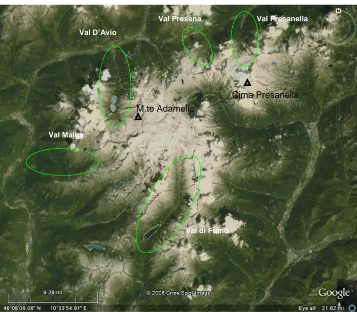
The Adamello-Presanella Group lies in the Southern sector of the Central Italian Alps (Rhetian Alps, 45° 54‘-46° 19‘ N; 10° 21‘-10° 53‘ E), covers an area of more than 1100 Km2 and hosts peaks exceeding 3500 m in elevation. The major peaks of the group are Cima Presanella (3557 m), Monte Adamello (3538 m) and Monte Carè Alto (3463 m) (Fig 2-1).

Other important massifs surround the Group: the Ortles-Cevedale Group to the North of the Val di Sole and Val Camonica, the Brenta dolomitic massif to the East of the Giudicarie Valley, and the Orobie Alps to the west of Val Camonica.

(9)

The Adamello-Presanella Group hosts about 100 glacial bodies, mostly lying in the northern and central sectors of the group; the Adamello Glacier, the widest glacier of the entire Italian Alps, develop on the summit area of the massif. The surface of the Adamello Glacier was 18,13 km2 in 1983 (Baroni & Carton, 1996), reduced to 17,24 km2 in 2003 (according to the analysis of the ASTER satellite image scanned on the 20th of June 2003; Ranzi et al. 2010). The glacialism is the morphogenetic phenomenon that most of all has contributed to the shaping of the landscape in the area. The numerous valleys descending from the central massif show a typical alpine morphology, with deep glacial troughs characterized by the succession of basins and steps, glacial shoulders, cirques, arêtes and horns (Fig. 2-3). In all the valleys glacial deposits of the major late glacial phases and of the LIA are present. Mass wasting and periglacial landforms are also common geomorphologic features scattered on the entire massif (Baroni et al., 2004).

Fig. 2-2. Administrative borders in the study area. Map scale 1:500000. Kompass

The five sampling sites involved in this study are located at the heads of five different glacial valleys surrounding the Central Massif of the Adamello-Presanella Group. The five valleys are included into the territory of two adjacent Natural Parks, the Adamello-Brenta

(10)

The former institution of the Adamello-Brenta Natural Park has been existed from 1967, but only in 1987 the institutive act was translated in laws focussed on the management and protection of the territory. It is the largest protected area of the Trentino region with an areal extension of 620,517 km2. It includes the Adamello and Brenta mountain groups, divided by Val Rendena and bordered by Val di Non, Val di Sole and Valle delle Giudicarie. The Adamello Regional Park was instituted in 1983; it completely includes the Lombardy side of the Adamello-Presanella Group, in the North-Eastern part of the Brescia province. It extends for 510 Km2 from the Tonale Pass to the Crocedomini Pass; the eastern side of its territory ends where Lombardy Region borders Trentino Region; westwards, its boundary is formed by the upper left side of the Oglio River, the fifth longest Italian river.

Fig. 2-3A panoramic view of the upper portion of Val di Fumo showing the typical U-shaped profile of the glacial valleys.

Geological lineaments

The Adamello-Presanella Group is mainly composed of volcanic rocks belonging to a large magmatic body, 670 km2, the largest of Alpine age, commonly referred to as "the Adamello batholith‖ (Callegari 1983, 1985). The emplacement of the batholith occurred in several stages throughout a succession of diverse intrusive episodes, from Eocene to the upper

(11)

Oligocene in the late phase of Alpine orogeny. The different intrusive episodes were evidenced by radiometric analysis performed by means of the Rb/Sr and K/Ar methods on mica and amphiboles of the igneous rocks (Del Moro et al. 1985). Within the batholith it is possible to distinguish four minor plutonic bodies (Bianchi et al. 1970, Dal Piaz, 1973), which, from south to north, are referred to as: Re di Castello, 40-42 Ma; Adamello, 34-36 Ma; Avio, 32 - 34 Ma; Presanella, 29-33Ma, divided into smaller units (Fig.2-4). The batholith intruded into the metamorphic rocks of the pre-Permian crystalline basement and the overlying volcanic and Permian-Mesozoic sedimentary sequences, belonging to the Southern Alps. This sedimentary sequence originally formed the continuous coverage of the batholith, and then was dismantled by erosion.

The batholith is located in a wedge of continental crust in the Southern Alps bounded by the Tonale and the Giudicarie fault lines. These fault systems belong to the tectonic system named lineament ―Insubrico‖ or ―Periadriatico‖ (Oligocene Age) that separates the domain of the Southern Alps from the ―Australpino Pennidico‖ domains to north. In particular, the Tonale line, direct-ESE OSO, is the tectonic boundary between the Southern Alps and the Austroalpine domain. The Giudicarie line directed NNE-SSW is situated within the Southern Alps and separate the Adamello block, and the Brenta Dolomites block (Callegari, 1983).

Fig. 2-4 Sketch map of the most important plutons of the Adamello batholiths (Mayer et al. 2003) The emplacement of the diverse plutons yielded to thermometamorphic phenomena that produced a wide metamorphic contact aureole involving all the rocks around the batholith along a wide band of about 1-2 km (Bianchi & Dal Piaz 1940, 1948).

(12)

The most widely outcropping rocks are tonalite, granodiorite and quartz diorite; Tonalite is characterized by a felsic composition, with phaneritic texture. Feldspar is present as plagioclase (typically oligoclase or andesine) with 10% or less alkali feldspar. Quartz is present as more than 20% of the rock. Amphiboles and pyroxenes are common accessory minerals (Bianchi et al., 1970; Callegari & Dal Piaz, 1973).

Vegetation lineaments

The shift in elevation that spans from the about 400 m a.s.l. of valley floors to the 3557 m a.s.l. of Cima Presanella, affects the structure, composition and distribution of all the vegetational ecosystems of the studied valleys. In terms of vegetation, according to the classification published by Pignatti in 1979, these altitudes correspond to the vegetation belts named Sub Atlantic, Boreal, ―alpica‖ and ―nivale‖.

Beech (Fagus sylvatica L.), that is considered one of the most representative trees of the sub-atlantic belt is not widespread or nearly absent in the studied valleys, probably because, in most part of the region, spruce (Picea abies (L.) Karst.) has been preferred to beech in the past for economic reasons (Dalla Fior, 1963). The absence of beech in the intra-alpine areas is indeed a renowned characteristic of the Alpine landscape (Ozenda, 1985; Theurillat & Guisan, 2001).

The prevailing forest cover is composed by acidophilic association (Vaccinio-Picetea, Pignatti, 1995), that means a predominance of spruce, accompanied by a thick undergrowth of blueberry (Vaccinium myrtillus L., Vaccinium vitis-idaea L.) and saxifrage (Saxifraga cuneifolia L.). Above 1800 m a.s.l. Larix decidua Mill.-Picea abies L. open stands (Vaccinio-Abietenion Oberd. 1962) dominate the forest cover. Moving upward to higher altitudes, spruce commonly give way to open mixed association of larch and stone pine (Larici-Pinetum cembrae Ellenberg 1963) with an undergrowth usually poor of species.

The upper tree-limit is located at about 1900-2000 meters, but isolated trees reach territories up to 2200 meters. The upper tree limit can be framed in a large phytocoenoses that has been studied for the first time by Pallmann and Haftter in 1933, Rhodoro vaccinietum. This association is composed by ericaceous short shrubs (Rhododendron, Vaccinium, Loiseleuria, Erica), that can sometimes be associated with tall shrubs (Pinus mugo L.) or trees (Picea abies (L.) Karst., Pinus cembra L., Larix decidua Mill.). Vegetation is poor in species but consists of a large number of phytosociological types (Pignatti et al. 1988).

(13)

Above this belt, between the upper mountain forest and the alpine belt, the forest cover is replaced by some bush-like growth-forms, genetically determined to resist to windy and cold climate. This typical formation, often referred to with the German term Krummholz or Krummholz belt (Braun-Blanquet, 1964), is constituted by typical twisted postured species. Some of the predominant species of this formation in the Alps, and in our study area too, are green alder (Alnus viridis DC), juniper (Juniperus nana L.), rhododendron (Rhododendron ferrugineum L.), Salix (Salix sp.) (Pignatti, 1995).

At these altitudes it is still possible to find single specimens of larch, pine and spruce ―advanced sentinels of the forest that would tend to rise, or survivor rear guard of the forest chased down by man for grazing lands "(transl. by G. Dalla Fior, 1963).

The dwarf shrub community Loiseleurio Cetrarietum is one of the dominating vegetation types immediately above the timberline (Grabherr, 1980) and is characterized by a dwarf shrub Loinseleuria procumbens (L.) Desv. (also known as Mountain Azalea), that is often associated with lichens (genera Cladonia and Cetraria) (Fig. 2-6).

Fig. 2-5 Loiseleuria procumbes (L.) Desv. forms herbaceous pillows on tonalite rock populated by lichens.

Above 2800-2900 meters, vegetation is dominated by alpine flora, pioneer vegetation consisting of lichens and bryophytes, and by various species with special adaptations to overcome the adversity of high mountains climate (Frattini, 1988).

At these altitudes on siliceous screes Cerastium uniflorum Desvío., Soldanella pusilla Baung., Doronicum cluded (All.) Tausch., Geum reptans L. and the glacier buttercup

(14)

Fig. 2-6. Ranunculus glacialis L., 2570 m a.s.l.

Fig. 2-7 Geum reptans L., 2570 m a.s.l.

We will consider more in detail the taxonomic characteristics and areal distribution of the conifer species involved in this study.

(15)

Larix decidua Mill. characteristics and distribution

The name of this species, Larix decidua, derives from the Celtic "lar"(= fat, for the abundance of resin). It is a tall tree that can reach 50 m. height, with sparse foliage and gray, thick, deeply furrowed bark (Farjon, 1990). Its altitudinal distribution ranges from 400 m a.s.l. in the Southern Alps to 2500 m a.s.l. in the central Alps (Gafta & Pedrotti, 1998).

Larch is the only European deciduous conifer and usually has upright stems and a deep root system. At the treeline European larch often form mixed association with Pinus cembra L., while at lower altitudes, with typycally less precipitation rates, they are often associated

with Pinus sylvestris L.

It is a long-lived species, and in the subalpine belt it can reach an age of up to 1000 years. In cross-section annual rings appear easily discernible in the sequence of earlywood and latewood, as well as the transition between duramen to alburnum that is generally sharp, resin canals are bordered by 8-12 secretory cells with thin cell walls (Schweingruber, 1993).

Due to its clearly marked duramen, the extreme longevity, the high sensitivity to climate, its presence in high-elevation mountain sites and its behavior as a pioneer species on denuded areas, European larch exhibits a good attitude to dendrochronological investigations (Serre 1978, Tessier 1986, Nola 1994). However, the use of this species in dendroclimatic studies, especially in the western sector of the Alpine Arch, has been questioned due to the action performed by an insect, the larch budmoth (Zeiraphera diniana Gen., Lepidoptera, Tortricidae). These defoliator insects, causing the loss of needles, negatively influence tree growth, and consequently number and width of annual rings.

Other natural factors that cause growth disturbances to this species in the alpine environment are those that commonly play an important role in all the high-altitude forests (mainly wind, frost, snow accumulation, processes and geomorphologic phenomena such as landslides and avalanches). Human-induced actions strongly influenced the dynamics of larch

Fig. 2-8 Some anatomical characteristics of

Larix decidua Mill Mod. from Dalla Fior,

(16)

forests because of domestic livestock grazing, forestry and timber use (Ozenda, 1985, Gafta et al. 1998). Assuming that the distribution of larch in the Alpine region had a maximum expansion and abundance in the interglacial periods, at present times this species has considerably narrowed its distribution area. The origin of this regression can be ascribed to two main reasons: climatic variations and anthropogenic pressure.

Climatic changes have had, throughout the Geologic Ages, an important role in the evolution of this species distribution and also at present times, climate continuously exert its strong influence. This influence does not appear immediately obvious, because of the slow evolution and the long response times of wooden cenosis (Fernaroli 1936).

Human pressure has been considerably intensified over time and, in our study area too, this influence is revealed in more active forest exploitation in general, and in particular of larch trees because of their value as lumber. This intense human impact on natural alpine vegetation has persisted until about the mid 19th century, when agricultural abandonment, reflecting a post war trend, took place in Western Europe (MacDonald et al 2000; Tappeiner et al. 2003). The land abandonment consequent to the decline of alpine farming produced the recent (MCPFE, 2007) forest invasion into former summer pastures and grasslands.(Walther et al. 1986; Didier, 2001)

On land denuded of vegetation, larch is one of the few tree species that, thanks to its biological characteristics (frugality, heliophilia and colonization aptitude within the domain of maximum distribution), is easily able to settle and rebuild a unique forest cover in a short time (Fernaroli, 1936). Pure larch wood stands represent the initial phase of a secondary succession tending towards the climax association, representing the initial stage of a consequent ecological succession.

The first vegetational association of the succession is the Laricetum pratosum (Rübel). In this first phase, because of the characteristics of heliophilia of this species and of its associations, a large number of species can contribute to the establishment of the herbaceous undergrowth. Actually, the undergrowth in this phase is not composed by species specialized for this association but mostly by ubiquitous species (Fernaroli, 1936, Pignatti, 1995). Afterwards bush-shaped species (nanophanerophyte) begin to settle into the larch wood.

The shrubby undergrowth is initially non-specific, but, in a second time, only a few species expand. At the end of this phase, undergrowth is commonly mostly composed by the following shrub species: Alnus viridis L., Rhododendron ferrugineum L., Vaccinium myrtillus L., Rosa sp., with a few other minor and mostly casual species (Fernaroli 1936, Dalla Fior

(17)

Picea abies ( L.) Karst. characteristics and distribution

Picea abies (L.) Karst. is an evergreen conifer with a shallow root system, its crown shape may widely vary. This variability is genetically and environmentally determined. Under optimal conditions, spruce can grow higher than 60 m, but in the mountain regions it usually reaches a height of about 20 m up to 30 m. In extreme conditions, like on windy hills, slopes and in avalanche channels or landslide sites with very thin soils, shapes and sizes can differ greatly from the norm (Dalla Fior, 1963; Farjon, 1990).

In mountain regions and especially in the Northern hemisphere this species forms a clearly marked forest belt. At lower altitudes spruce is associated with beech, and in areas with low rainfall rates with Pinus sylvestris L. and Pinus mugo Turra. Thanks to the excellent technological properties of its wood, it has found wide applications in the industry, and it has been planted in many areas outside its natural range.

In cross section there is not a visible distinction between hardwood and sapwood and wood appears yellow-straw coloured with silk reflexes. The growth rings are easily discernible, with frequent resin ducts, and the latewood less intensely coloured than in larch (Schweingruber, 1993). The natural range of this species occupies most of the territory of the Trentino-Alto Adige region, except in the most oceanic area situated at its southern limit, however, because of the large extent of areas affected by forestry operations, it is difficult to distinguish natural and primitive stations (Fig.2-10). In particular, the Val d‘Amola, Val di Ledro, Valle del Sarca, Val d‘Adige, Val Ronchi and Vallarsa remain outside its natural range, which is almost complementary to the oak (Quercus petraea (Mattuschka) Liebl.) natural range (Gafta & Pedrotti, 1998).

Fig. 2-9. Some anatomical characteristics of

Picea abies (L.) Karst., here reported the old

scientific denomination Picea excelsa L. mod from Dalla Fior , 1963.

(18)

Fig. 2-10 Natural distribution of Picea abies (L.) Karst. in the Trentino-Alto Adige region (southern boundary) as reported in Gafta & Pedrotti., 1998

(19)

3 Materials and methods

Climate data

High-mountain areas are commonly poor in meteorological stations providing long and uninterrupted series of climate variables. Also in our study area there are not suitable long meteorological series coming from nearby high-elevation meteorological stations.

The only two meteorological stations located at an altitude > 1400 m a.s.l., that have recorded the longest climate data series in the area, are situated on the mountain pass named ―Passo del Tonale‖ (1880 m a.s.l.). These two stations have registered data from 1987 to present, but the climatic series derived from these records are full of gaps with whole years missing (data from Meteotrentino http://www.meteotrentino.it/) (Tab. 3-1).

All the other available and examined stations in the area provide shorter and non continuous series. For instance, the ―Cima Presena‖ Station, that is the station located at the highest elevation, 2730 m a.s.l., recorded data only for a very short time period, from January 1995 to December 2005. Furthermore, climate series coming from ―Cima Presena‖ station present many gaps each year, except for 1999, the only one year with a complete and uninterrupted succession of data (data from Meteotrentino and from IASMA ―Istituto Agrario San Michele all‘Adige‖ http://www.meteotrentino.it/) (Tab.3-1).

Because of the poor quality and the short lengths of these instrumental climate data, we decided to refer in this study to the gridded data set provided by the HISTALP project (Auer et al 2007, Böhm et al. 2001, Böhm et al. 2009, http://www.zamg.ac.at/histalp). The HISTALP database consists of monthly homogenised records of temperature, pressure, precipitation, sunshine and cloudiness for the ‗Greater Alpine Region‘ (GAR, 4–19 °E, 43–49 °N, 0–3500m a.s.l.). In this dataset the longest temperature and air pressure series extend back to 1760, precipitation to 1800, cloudiness to the 1840s and sunshine to the 1880s.

We used the gridded dataset of temperature and precipitation anomalies referred to the grid point 10°N, 46°E.

Monthly gridded temperature data span from 1760 to 2007 (247 years) and monthly gridded precipitation data from 1799 to 2003 (204 years). Temperature series are differentiated in temperatures recorded from high (>1400 m a.s.l.) and low (<1400m a.s.l.) altitude stations (Tab.3-2).

(20)

Temperature and precipitation anomalies refer to the Twentieth Century mean (1901-2000) and were derived only for homogenised data, both for the monthly temperature series (2004-11 release); and the monthly precipitation series (2004-2008 release) (Auer et al 2007).

Pas so T o n ale 1 Pas so T o n ale 2 Val d i Gen o v a C im a Pre sen a L ag o d‘ Ar no L ag o d‘ Av io L ag o Salar n o Pan tan o d‘ Av io Ma lg a B is sin a M alg a B o az zo Po n te Mu ran d in R if . Ag o stin i Pra d alag o T o rr en te Ar n ò C am p o C ar lo Ma g n o 1978 1979 1980 1981 1982 1983 1984 1985 1986 1987 1988 1989 1990 1991 1992 1993 1994 1995 1996 1997 1998 1999 2000 2001 2002 2003 2004 2005 2006 2007 2008

Tab. 3-1 Extension of historical temperature data series derived from high-elevation meteorological stations in the study area. Years with incomplete series are marked with a diagonal line.

Temperature Precipitation

High >1400m a.s.l. Low <1400m a.s.l.

1799-2003

1818-2007 1760-2007

Tab. 3-2 Extension of temperature and precipitation data for the grid point 10° N, 46° E (HISTALP Dataset, Auer et al 2007)

(21)

Tree-ring data

Field collection and sampling strategy

This study is based on tree-ring cores and cross-sections collected during three different summer field trips carried on in 2005, 2007 and 2008.

The five sampling sites are located at the heads of five different glacial valleys surrounding the Central Massif of the Adamello-Presanella Group and are situated at the northern, western and southern sides of the Adamello-Presanella Group (Fig. 3-1, Tab. 3-3). The Italian names of these five valleys (used to indicate the five sampling sites in the following text) are Val Presanella, Val Presena, Val d‘Avio, Val Malga and Val di Fumo.

In detail, Val Presanella, Val d‘Avio and Val Presena are S-N oriented and are located on the northern side of the Massif, Val Malga has an EW orientation on the western side of the massif and Val di Fumo is NS oriented and located in southern side of the massif.

Fig. 3-1 spatial distribution of the five valleys where are located the five sampling sites.

Val Presanella Val Presena Val D’Avio Val Malga Val di Fumo M.te Adamello Cima Presanella

(22)

The five sampling sites are mostly geobotanically homogeneous, with some minor differences, and the sampled trees are located close to the upper treeline, at an elevation range of 1980-2130 m a.s.l.

The alpine treeline is an extreme environment for plant life and has been demonstrated that plant growth at high-elevation sites is directly or indirectly limited by temperatures (Körner & Larcher 1988, Körner, 1998). Preferring for our purposes climatically-stressed sites, we chose these high-elevation sites for minimizing the non-climatic influences on tree growth, such as stand competition or insect-induced defoliation.

One of the main problems we met during the sampling campaigns was to find very old trees. The current vegetational composition at the tree line in our study area is affected by the natural and human-induced disturbances that have characterized these ecotones over the centuries (Anfodillo & Urbinati, 2001). Within the most recurrent disturbances in the study valleys, we especially found grazing and wood exploitation for charcoal and lumber production. Moreover, at the beginning of the last century, on the Adamello-Presanella area, the human impact on treeline was also determined by the fighting of World War I between the Italian and Austrian armies (Ronchi, Q., 1927; Viazzi, C. & Cavacicchi, 1996; Viazzi, C., 1981). More recently, the building of dams for hydroelectric power production (in Val d‘Avio and in Val di Fumo) and the development of some ski tracks (in Val Presena) amplified human disturbance on the high-altitude natural environment.

At the present time the treeline population in the five sampling sites mainly consists of larch (Larix decidua Mill.) in pure or mixed formations with stone pine (Pinus cembra L.) in a variable percentage (―larici-cembretum‖ association, Pignatti et al. 1988, Pignatti, 1995). In Val Presanella and in Val Malga larch is associated to a limited number of Norway spruce (Picea abies (L.) Karst) (Figs 3-2 and 3-3).

Due to the purpose of this study, sampling has been performed in order to remove as much as possible non-climatic factors on tree growth (Cook & Kairiukstis, 1990).

In order to minimize possible effects of stand competition, only dominant and sparse trees with undisturbed canopies have been sampled. A special attention was given in choosing the correct trees, avoiding those plants showing external evidences of non-climatic growth disturbances, such as lightning scars, broken branches or crowns, buried stem bases.

(23)

Fig. 3-2 A view of the upper treeline in Val Presanella. The alpine hut (Rifugio Denza) is located at 2300m a.s.l.

Fig. 3-3 A view of the upper tree-line in Val di Fumo. The upper sparse trees are located at about 2100 m a.s.l.

(24)

Site Species Mean altitude (m) Latitude N Longitude E

Avio LaDe, PiCe 2150 46°10‘ 10°28‘

Fumo LaDe 1990 46°05‘ 10°34‘

Presanella LaDe, PcAb 1910 46°25‘ 10°65‘

Presena LaDe 2160 46°23‘ 10°60‘

Malga LaDe, PcAb 1850 46°07‘ 10°25‘

Tab. 3-3 Site characteristics

At least two cores from opposite sides of each living tree were taken, following the standard sampling procedures (Stokes & Smiley, 1968). Cores were extracted using an increment borer at breast height (~ 1,30 m from the ground level), coring horizontally and at 90° with respect to the slope direction, in order to avoid possible compression wood (Fig 3-4).

(25)

Fig. 3-5 An increment borer in a larch stem

All the cross-sections were taken by means of a chain saw. They all come from only one of the five sampling site (Val Presanella). The most part of the cross-sections have been sawn from uprooted trees found along three different snow-avalanche channels (Fig. 3-5).

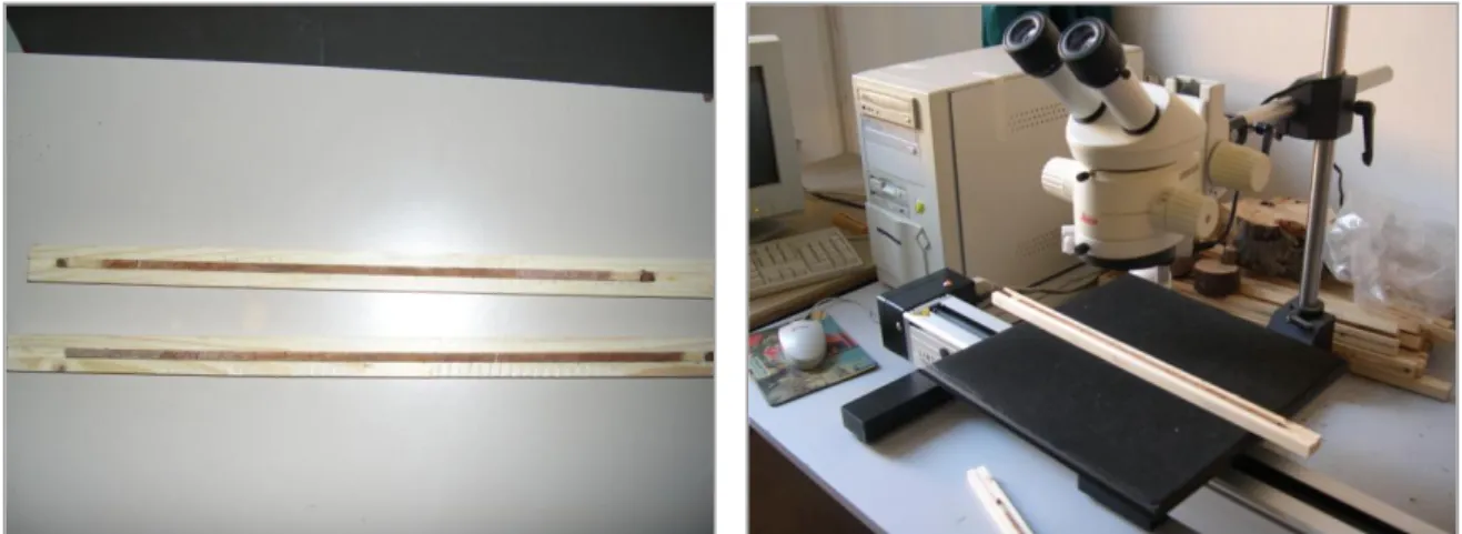
Fig. 3-6 Two of the twenty-six cross-sections sawn by uprooted trees analysed and dated in this study, here shown as they were before of the sanding procedures.

Twelve cross-sections have been sawn from beams of nine isolated barns (locally named ―maso‖ or ―malga‖), little rural alpine houses mainly used as stalls and haylofts. They are all located in Val Vermigliana, (Fig.3-6, 3-7 and 3-8) of which Val Presanella is a lateral valley. We want to explore the possibility to use these samples in order to improve the sample replication in the earlier part of the Presanella mean site chronologies. The use of historical materials in Dendroclimatic studies is usually avoided because of the uncertain provenance of

(26)

timbers utilized in historical buildings. Nevertheless, as reported in Wilson et al (2004) ―in situations when it can be shown that historical timbers are locally derived from climate-sensitive stands, these records may have a considerable potential use in developing and extending dendroclimatic reconstructions‖. In our case some oral evidences testify that the provenance of timber used in the barns‘ construction is likely to be close to our sampling area.

Fig. 3-7 Location of the sampled farmsteads

Fig. 3-8 “Maso Cavel”, one of the sampled rural buildings.

Val Presanella

(27)

Fig. 3-9 Four of the twelve cross-section coming from farmstead’s beams analysed and dated in this study.

The geographical position of each tree has been marked using a GPS (Global Position System) device and reported in a GIS database (Figs 3-10 to 3-14).

The tree-ring collection is constituted of 389 samples:

 350 cores from 169 trees (Larix decidua Mill., Picea abies (L.) Karst and Pinus cembra L.)

 38 cross-sections (Larix decidua Mill., 12 disks from historical material and 26 disks from uprooted trees).

(28)

(29)

(30)

(31)

(32)

(33)

Samples preparation and tree-ring measurement

In the laboratory each core has been dried and mounted with vertical fibers on wooden supports. A transversal surface of the cores was then cut with a sharp cutter blade in order to make tree rings clearly visible (Ferguson, 1970; Pilcher, 1990).

The full disks surfaces were sanded with an electric belt sander on which were mounted sand papers of various grain sizes, from coarser to finer. The core surfaces were instead sanded by hand with simple sand paper of progressively finer grain sizes.

Tree-ring widths were measured with a precision of 0.01 mm using a LINTAB increment measuring table (RinnTec) associated with the program TSAP (Time Series Analysis Program, Rinn, 1996) (Fig. 3-15).

For each cross-section from three to four radii were measured, preferring undamaged directions and excluding those parts showing anatomical irregularities such as compression wood, suppressions, wound tissue, scars or knots.

When needed, the contrast between wide earlywood cells and small latewood cells was enhanced by rubbing chalk or water on the wood surface. Broken cores or cores with evident signs of mechanical disturbances were discarded.

Fig. 3-15 cores mounted on wooden supports ready for measuring and Lintab increment measuring table

Larch Bud Moth attacks correction

In the European Alps insect outbreaks are not so decisive in defining forest dynamics as in other forest ecosystems (e.g. the North-American conifer forests, Swetnam et al 1995, Swetnam & Lynch,1993). Nevertheless European larch trees are periodically severely affected by the attacks of a Lepidoptera, the gray larch bud moth (Zeiraphera diniana

(34)

Guénée, Lepidoptera: Tortricidae). Zeiraphera diniana (here referred to as LBM) is a foliage-feeding Lepidoptera that is widespread throughout the European Alps (Baltensweiler, 1985, Rolland et al 2001, Weber, 1997). The pullulations of this insect occur cyclically approximately every 8–9 years in the subalpine pure or mixed larch forests (Baltensweiler et al 1977; Baltensweiler and Fischlin 1988; Bjørnstad et al. 2002).

The effect of these attacks is the partial or complete defoliation of the trees, causing the production of an exceptionally narrow annual ring that sometimes is difficult to distinguish (Pignatelli & Bleuler 1988; Schweingruber, 1996).

For the current study, LBM effects are regarded to as noise and must be corrected in order to minimize the effects of non climatic (negative) outliers on the resulting mean site larch chronologies.

To detect years with LBM induced defoliation usually a comparison between host and non-host species is performed (Swetnam et al. 1985; Swetnam & Lynch 1993). Unfortunately, we had not non-host species to compare with larch in the whole sampling sites, because sampled spruces and stone pines, when present, were always younger than larch trees.

We identified years of LBM attacks with the simplest method, based on the accurate observation of the anatomical characteristics of the tree rings. Tree-ring features, as total ring-width or colour and thickness of latewood, are in fact important indicators of possible insect attacks and consequent tree defoliation (Filion et al. 1986; Pignatelli & Bleuler, 1988; Schweingruber et al. 1996; Liang et al. 1997). In our larch samples the typical growth pattern produced by LBM attacks was almost always clearly visible (Fig. 3-16).

Fig. 3-16 tree-ring growth patterns produced by LBM attacks on two samples coming from the Val di Fumo site, the red dots indicate the year of defoliation.

(35)

To correct the low width values of the years of defoliation, we have followed Büntgen et al. 2006 (b). In detail, the affected rings width values were removed and substituted with a statistical estimate derived from the mean of the remaining unaffected rings.

Chronology development and statistics

The measured growth series coming from different radii of the same cross-section or from different cores of the same tree were visually and statistically cross-dated (Fritts, 1976, Fritts & Swetnam 1986) using the program TSAPwin. Once checked the correct dating and removed the possible measuring or dating errors, a mean growth series was calculated for each tree (Cook and Kairiukstis, 1990).

Two different statistical parameters were used to check out the correct cross-dating between the tree-ring series: t-values relating to correlation coefficient (Baillie & Pilcher, 1973) and the Gleichläufigkeit (GLK; year-to-year agreement between the interval trends of two time series; Schweingruber, 1988) computed by the TSAPwin software.

Only those time series longer than 100 year were used in the successive analysis and only the time series with a satisfying mean site correlation (GLK > 0,60) and t-values (t > 2,5) were retained for computing mean site chronologies.

To absolute dating the cross-sections coming from uprooted trees and historical material, the floating undated mean growth series were cross-dated against the dated tree-ring series of the living trees of the Val Presanella site (remember that all the dead material comes from that site).

The correct dating of the historical material has been further checked, cross-dating the floating mean series against four of the existing larch chronologies for the Alpine area, used as independent references: Eastern Alps (Italy, Bebber, 1990); Fodara Vedla (Italy, Hüsken, Schirmer, 1993), Obergurgl (Austria, Giertz, ITRDB, International Tree-Ring Data Base); Ötztal (Austria, Siebenlist-Kerner, 1984). For these samples we have used a more restrictive dating criterion and considered as parameter of a reliable dating quality a t-values higher than 4.5 (Baillie, 1982).

The correct cross-dating between measured tree-ring series was further verified using the program COFECHA (Holmes, 1983; Grissino-Mayer 2001), which identifies segments within each ring-width series that may contain erroneous cross-dating or measurement errors.

Because of the greater number of available larch samples, and due to the better intercorrelation between their ring-width series, all the five mean site chronologies are made

(36)

Mean site chronologies were calculated using the program ARSTANwin (Cook and Holmes 1984; Cook 1985). This program operates a standardization of the time series prior to average them in a mean chronology, allowing also the selection of detrending methods and autoregressive modeling.

Standardization of raw tree-ring series is a basic operation in treating tree-ring data (Fritts, 1976). It allows to correct tree-ring width for their systematic non–climatic change due to tree age (the so called age trend) and to average the standardized obtained values in a mean function. Moreover it permits to adjust the series for different growth rates that are caused by individual differences in the overall rate of growth (Cook & Kairiukstis, 1990).

This process transforms ring-width values in stationary dimensionless indices that have a defined mean of 1.0 and a homogeneous variance. Dimensionless indices are computed by dividing the observed ring-width value by the one predicted by a function. The standardized indices of individual trees are averaged to compute the mean site chronology.

There are numerous ways to standardize tree-ring widths, more or less conservative, and the choice depends on the finalities of the different tree.-ring analysis that may be performed. Due to the purposes of this study, with the aim to enhance the climatic signal into the five tree-ring site chronologies, we have chosen a double detrending method (Cook, 1985).

First, a negative exponential curve or a linear regression line is fitted to the ring series, afterwards, each value of the time series where divided by the value predicted by a cubic smoothing spline function. The wave-length of the spline was fixed at 67% of the mean length of the series, with a 50% frequency cut-off, thus removing the non-climatic trends due to tree age, to tree size, and to stand dynamics effects (Cook & Peters 1981; Cook & Briffa, 1990). Individual indexed series were then computed into the mean site chronology by means of a bi-weight robust estimate of the mean, in order to reduce the effects of statistical outliers (Cook 1985; Holmes 1994).

Several statistics have been considered to evaluate the validity of the resulting five mean site chronologies.

Mean sensitivity, measures the relative differences in width from one tree-ring to the next. Douglass (1936) defined in this way this statistic: ―mean percentage change from each measured yearly ring to the next‖.







         1 1 1 1 2 1 1 t n t t t t t x x x x x n Ms (Fritts, 1976)

(37)

Where x is each ring width, Ms values range from 0, if all rings are the same size, to _t 2 if a zero value occurs next to a non-zero one in the time sequence.

The correlation coefficient (r) is a measure of the degree of linear relationship between two variables. In Dendroclimatolology it is also used to measure the association between time series, e.g. two chronologies or a chronology and a climate series.











x y n t t y t x t xy s s n m y m x r 1 1    



  (Fritts, 1976)

Where m_x,my,s , x sy are the means and the standard deviations of the two set of data

and n is the sample size. It can range from +1 that indicates perfect agreement to -1 that indicates inverse agreement.

Chronology signal-to-noise ratio (Wigley et al. 1984) has been used to evaluate the relative strength of the common variance signal in the five tree-ring chronologies

 

r r N SNR   1 (Cook el al 1990)

Where ris the mean interseries correlation between trees and N is the number of trees. Since our chronologies are composed by individual series of different lengths, it was important to assess the adequacy of replication in the early years of their temporal extension, for this purpose we referred to the subsample signal strength (SSS) (Wigley et al 1984). It allows quantifying how well a chronology based on a subset of t‘ trees estimate a larger t series chronology.

 





 



t r



t r t t SSS 1 ' 1 1 1 '      (Wigley et al, 1984)

Where t and t' are the number of tree-ring width series in the sample and in the subsample and r is the mean interseries correlation. Usually, the period used for calibrating tree-rings against climate parameters is the time when the chronology is formed by the highest number of individual series. SSS allows evaluating the possible loss of reconstruction accuracy that occurs when a chronology made up of a few series is used to reconstruct past climate, considering that the used transfer function usually derives from a chronology with a greater number of series (Wigley et al., 1984). We decided to limit our chronologies to the time period with SSS > 0,85. This threshold has been indicated by Wigley et al. (1984) to sufficiently ensure only a small loss of explained variance due to the reduced number of samples in the early part of the chronologies.

(38)

First-order autocorrelation. In time series, most of all when biological systems are involved, it is possible that one value is affected by the preconditions of the other values of the series (Fritts, 1976). The first-order autocorrelation indicates how much each value of a series is correlated with the preceding term. When the first-order autocorrelation is close to 0, each yearly value is independent of the one before, when it is close to 1, it means that each yearly value is largely influenced by the one before.

The program ARSTANwin allows to compute three different version of the mean site chronologies: a Standard Chronology, where standardized tree-ring index series are combined into a mean value function of all series, a Residual Chronology that is computed in the same way of the standard version, but using the residual series resulting from an univariate autoregressive modelling, fitting an autoregressive order to each series, and an Arstan Chronology computed using the autoregressive coefficient selected into a multivariate autoregressive modelling and reintroducing the pooled autoregressive model into the residual chronology (Cook & Holmes, 1984). In order to establish the proper version of the five mean site chronologies to use in the successive dendroclimatic analysis, that is whether we should use the standard or residual version of the chronologies derived from the standardization procedures, an autocorrelation analysis has been performed and the first-order autocorrelation has bee evaluated (Box & Jenkins, 1976) (see next chapter for detail on this analysis results).

In order to highlight similarity between the five mean sites chronologies, hierarchical cluster analysis was performed on their common period (1818-2004), producing clusters of the five sites (Leonelli et al, 2009). The five variables were grouping according to the average linkage method and the Euclidean distance was used as a measure of similarity.

The four residual chronologies showing the higher inter-correlation values (Avio, Presanella, Fumo, Presena) were then chosen for successive analysis.

Climate/tree-rings relationship

A fundamental phase in a dendroclimatic analysis is the recognition of the prevalent climatic features that affected tree growth in the studied area. The most commonly used statistical models in delineating climate/tree-rings width relationship are called correlation function and response function (Fritts et al., 1971; Blasing et al., 1984).

(39)

In the both methods a sequence of coefficients are computed between the tree-ring chronology and the monthly climatic variables, which are ordered in time from the previous-year growing season to the current-previous-year one.

In the correlation functions the coefficients are univariate estimates of Pearson‘s product moment correlation (Arnold, 1990), and the function is the temporal sequence of correlation coefficients between the tree-ring chronologies and the monthly climate variables. The response function is a form of principal component regression and the coefficients are multivariate estimates from the principal component regression model (Fritts, 1976, Briffa and Cook, 1990a).

These two models take for granted that climate/tree growth relationship is stable in time, but in this way time-dependent changes of the climate/tree growth relationship are not considered (Biondi, 1997). Actually, response and correlation function may vary if the relationship we are trying to capture is not stable through time or if the original response function doesn‘t contain all the important predictor variables.

If a wealth of long climate series is available it is possible to check the stability of the relationship by calculating response and correlation functions for successive blocks of time. Therefore there are few locations, and our study area is not one of these, where a sufficient length of climate records is suitable and allows calculating successive non-overlapping response and correlation functions. For these reasons, for capturing the dynamical variability of climate signals in tree-ring chronologies the moving correlation function (MCF) and the moving response function (MRF) are now widely used. These two methods use a fixed number of years that is progressively shifted over time to calculate response and correlation coefficients (Biondi, 1997). They are based on a bootstrapping method, where the moving intervals iterate the bootstrapped correlation and response function for different time period (Fritts and Guiot 1990; Guiot, 1991).

In this study climate/growth relationships have been tested using the standard correlation function (CF) analysis to assess climate–growth relationships (Fritts, 1976) and MCF to test their stationarity and consistency over time, by applying the software package DENDROCLIM2002 (Biondi 1997; Biondi and Waikul, 2004). Each bootstrap estimate was obtained by generating 1000 samples and running numerical computation on each sample. For each interval, the median coefficients estimated from the 1000 bootstrap samples are reported in the output, and are plotted only if they are significantly different from 0 at the 0.05 probability level.

(40)

The monthly climate analysis was performed, both for mean monthly temperatures and for total monthly precipitations, choosing 18 climate variables (predictors), from July of the year before growth (t-1) to December of year (t) of growth. The analysis of residual chronologies/monthly mean temperature relationship was carried on with temperature data coming both from high elevation meteorological stations (>1400 m a.s.l.) and from low elevation stations (<1400 m a.s.l.). To provide a sufficient number of degrees of freedom, the length of the calibration period (60 years) was consistently higher than the number of predictors, which were 18 in this study. We performed this analysis with all the five mean site residual chronologies and with a composite chronology (All). The All chronology was obtained averaging the mean site residual chronologies except the Malga chronology that has revealed the lower correlation values with the other four.

To assess any intercollinearity present in the correlation function parameters, we performed response function analysis, using the same climatic variables and calibration period length. All the analysis was performed over the 1878-2004 period.

Extreme weather events have become more frequent in Europe during the last decades (Klein Tank and Können, 2003). To highlight the answer of the Adamello-Presanella larch ring chronologies data set to an exceptional climate event, we have checked out how tree-ring indexes are correlated to the heat wave of summer 2003 (Pilcher & Oberhuber, 2007; Leonelli et al., 2009). Year 2003 was an extraordinary year from the climatice point of view and mean summer temperatures of central Europe exceeded the 1961–1990 mean by ca. 3,8oC (Beniston, 2004; Luterbacher et al., 2004; Schär et al., 2004)

Climatic variables reconstruction

With the aim to test the efficiency of the computed larch mean site chronologies for climate reconstruction purposes, we have conducted a first tentative of climate reconstruction using the transfer function method (Fritts, 1976; Briffa et al. 1982; Fritts & Guiot, 1990).

In the transfer function computation the tree-ring chronologies are the predictors and the climate parameters the predictant.

The procedure that estimates the statistical tree-rings growth/climate relationship is called calibration. This statistical procedure involves calculating of a set of regression coefficient of a linear regression equation representing the relationship between climate parameters (temperature or precipitations) and a set of tree-ring chronologies (Briffa, 1982).

(41)

In a second time ―growth records are transferred in the reconstruction of climate‖ (Fritts, 1976), in other words, the coefficients are applied to tree-ring data to obtain estimates or reconstructions of climate parameters (Fritts & Guiot, 1990).

A correct calibration procedure requests some important assumptions, such as the normal distribution of data (both climate and tree-ring chronologies) and the absence of autocorrelation. These are essential premises because the presence of outliers can distort the significance testing and the interdependence of observation in time can reduce the number of degrees of freedom used for statistical significance testing (Fritts & Guiot, 1990). To avoid as best as possible these potential problems we have proffered a particular care in evaluating normal distribution of tree-ring data and climate parameters, and we have chosen to use the residual chronologies as predictors because of their lower values of autocorrelation (see next chapter for details).

We used histograms to compare the frequency distributions of the climate data and the predictors.

To further asses the distribution of tree-ring data and in order to measure how well the data follow the normal distribution we performed a statistical test for normality, the Anderson-Darling test (Anderson & Darling, 1950).

The Anderson Darling test compares the empirical cumulative distribution function of sample data with the distribution expected if the data were normal. If the observed difference is sufficiently large, the test will reject the null hypothesis of population normality.

The hypotheses for the Anderson-Darling test are: H0: The data follow a specified distribution. H1: The data do not follow a specified distribution.

The better the distribution fits the data, the smaller this statistic will be, if the p-value for the Anderson-Darling tests is lower than the chosen significance level (0.05 in our case), then the data do not follow the specified distribution.

To clearly represent the fitting to normal distribution of our tree-ring data we have used probability plots where each value was plotted vs. the percentage of values in the sample In any regression technique it is important to be able to test the regression equation using an independent data set. This independent testing procedure, called verification, allows assessing if the modelled growth/climate relationship obtained for the calibration period are valid over an independent time period. Verification is established when the reconstructed values derived from the independent predictors set is similar to the independent predictant set

(42)

particular climate/tree-growth relationship is not occasional, and that the subsequent reconstruction actually represents real conditions.

In this study we have used the transfer function method with a single predictant variable. The climate parameters involved in the reconstruction are those showing better results in the MCF and MRF analysis.

In order to use as best as possible the common signal strength of the five chronologies we have discarded those chronologies (Malga chronology, see next chapter for details) presenting the lower climate/tree growth correlation and the weaker correlation with the other chronologies.

The four mean site residual chronologies chosen for the reconstruction start in different years and their different time span imply a reduced replication in the earliest period of the time series. Considering the different length of the chronologies, it is strategically important to correctly select the appropriate reconstruction technique and the more proper calibration/verification periods.

With the aim to use the full length of the tree-ring chronologies and not limiting the reconstruction to their common period, we decided to compute a series of nested principal component regression models (Meko, 1997; Cook et al., 2002, 2003). The individual calibrated models are developed using all available predictors for each time period, and are then merged together, so that a near-maximum number of predictors is used to estimate climate variables back in time. The climate variables interested by the reconstruction are those presenting the better results in response and correlation functions analysis.

We have defined three models limited by the starting year of each chronology, in fact the starting year of each chronology represents in our tree-ring data set an important point of change in the availability of the tree-ring series, and then we have used the PC calculated for each nest as the potential predictors in the nested time period. The nested multivariate regression models assure that each time period is represented by the corresponding regression model with the greatest number of available data (Meko, 1997, Briffa, 1988).

Principal component analysis

When, as in our case, the number of predictors is higher than one it is opportune to reduce them in a minor number of candidate principal component (PC) predictors (Fritts, 1976, Peters, 1981, Briffa et al. 1982; Briffa et al., 1988).

(43)

climatic parameters sensu lato or more precisely summer temperatures. This method has demonstrated in many studies to be superior of simple correlation analysis (Frank & Esper, 2005b, Cook et al 2003).

With the principal component analysis the predictor variables are transformed into a new set of orthogonal and uncorrelated variables (eigenvectors or principal components) and a smaller number of transformed variables may be required to obtain the regression relationship. High-order principal components whose cumulative variance does not exceed a predefined threshold can be rejected, and, at the end, the amplitude time series for the PC predictors are regressed individually against the predictand data series (climate parameters) in the calibration process. As seen above, ―to calibrate‖ means to develop a regression model (the transfer function) that we can use to convert tree ring values (or their PC) into climate variables values. In our case, in the calculation of transfer function, PC eigenvalues derived from tree-ring residual chronologies are the predictors and the climate variables are the predictand.

We decided to apply this method, even with a small number of chronologies to preserve the climatic common signal over the four chronologies used in the reconstruction.

In a first step a multiple regression technique has been performed to convert tree-ring chronologies time series (in our case residual chronologies) into their principal components, in view of the fact that we have chosen chronologies on the base of their good intercorrelations, it was probable that a lower number of eigenvalues expresses most of the variance. The PC rejection criterion follows the most common approach, to deciding the appropriate number of factors we have generated a scree plot. The scree plot is a two dimensional graph with factors on the x-axis and eigenvalues on the y-axis, in this manner it is possible to highlight which factors account for the most part of the variance. Several other plots were realized to further verify the scree plots results. The Score plot for first 2 components plot which plots the scores for the second principal component (y-axis) versus the scores for the first principal component (x-axis); the Loading plot for first 2 components: plots the loadings for the second component (y-axis) versus the loadings for the first component (x-axis). A line is drawn from each loading to the (0, 0) point; the Biplot for first 2 components plots an overlay of the score and loading plots for the first two components.

Even if this approach to selecting the number of factors involves a certain amount of subjective judgment, our choice was further verified using the Kaiser-Guttman rule that remove all those components for which the eigenvalues are <1.