SCUOLA DI INGEGNERIA INDUSTRIALE E
DELL’INFORMAZIONE
Laurea Magistrale In Ingegneria Meccanica
A discrete event simulation study for optimization
of an automated guided vehicle (AGV) system
Supervisor: Prof. Marcello URGO
Company supervisor: Ing. Francesco POCCHIA FEBBRARIELLO
Simone MALFER
8778591 Index
1 Problem presentation ... 5
1.1 Overview ... 5
1.2 Introduction ... 6
2 Company and methodologies ... 9
2.1 The company ... 9
2.2 World Class Manufacturing ... 11
2.3 The origin of WCM ... 12
2.4 WCM pillars ... 14
2.4.1 Focused Improvement ... 15
2.4.2 Logistic Pillar ... 17
2.4.3 Cost Deployment Pillar ... 19
3 State of the Art ... 21
3.1 Input Data Analysis... 21
3.1.1 Chi-squared test ... 21 3.2 Simulation techniques ... 22 3.2.1 Focus on simulation ... 24 3.2.2 Method selection ... 25 3.2.3 Computer Simulation ... 26 3.2.4 Important aspects ... 27
3.2.5 Different type of simulations ... 28
3.3 Warm-up period ... 29
3.3.1 Welch Method ... 30
3.4 Notations and methods ... 31
3.5 Bonferroni approach ... 32 3.6 Subset selection ... 33 4 Problem Statements ... 35 4.1 Process description ... 35 4.2 Process overview ... 39 4.3 First phase ... 40 4.4 Second phase... 42
2
4.6 Processing times ... 43
4.7 Routes and distances ... 48
4.8 The model ... 50 4.9 Policies ... 52 4.9.1 Preconditions ... 52 4.9.2 Position ... 53 4.9.3 Number of carts ... 55 4.9.4 Software ... 56 4.9.5 Preferred parking ... 57 4.9.6 Priorities ... 58 4.10 Scenarios ... 59 4.11 Logic flowchart ... 62
5 Definition of the DES Model ... 65
5.1 Input data analysis ... 65
5.1.1 Application of Chi-square test ... 68
5.1.2 The adopted solution ... 68
5.2 Building the model ... 71
5.2.1 Introduction ... 71
5.3 Model’s development ... 73
5.3.1 Product creation ... 73
5.3.2 First Batching process ... 75
5.3.3 Second line ... 76
5.3.4 Third line ... 77
5.3.5 Transporters ... 78
5.3.6 Network Links ... 80
5.3.7 Vehicle’s logic ... 81
6 Application to the industrial case ... 83
6.1 Identification of the Warm up period ... 83
6.2 Welch method application ... 85
6.3 Replication parameters ... 87
6.4 Output ... 88
3 6.6 WIP ... 92 6.7 AGV utilization ... 94 6.8 Subset selection ... 96 7 Final considerations ... 97 7.1 Model limitation ... 97 7.2 Conclusions ... 98 8 Bibliography ... 101
5
1 Problem presentation
1.1 Overview
The thesis is carried out during an experience of a seven months internship in Magneti Marelli s.p.a. I developed my thesis in the Corbetta plant, the head-quarter of the company. Magneti Marelli has 8 business unit and in Corbetta there are Electronic System, Motorsport, Powertrain and After Market Parts and services. My focus will be around a logistic issue regarding the Logistic pillar of WCM (World Class Manufacturing), a methodology that will be presented in this document.
In the Corbetta plant there are AGVs (Automated Guided Vehicles) used to move raw material from the warehouse to the processing lines. My mission was to implement new routes for semi-finished products that nowadays are moved by operators in the powertrain area of the plant, assessing their KPIs.
During the development of this document the methods of WCM will be described, as the pillars involved, to provide how this target has been attentioned. As a WCM specialist I was mainly concerned with the Focused Improvement pillar that aims at attacking a particular loss affecting the overall cost of transformation.
The company and the methodologies of the production system used will be introduced at the beginning of the document to clarify the environment in which this study was conducted. The pillars mainly involved in the implementation of this study will be presented in order to understand the way in which the company operates.
The real system will be presented to let the modelled system to be introduced from a broader point of view, as well as the process steps of the product will be explained to illustrate how the data were obtained and therefore the objectives to achieve. The methodologies for estimating the performance of the real system will be introduced by literature, then applied to data coming from the production system, taken directly from the production lines. Subsequently, the reasons that led to the evaluation of the system through simulation will be illustrated, providing a description of the limits and potentialities associated with this methodology.
6
The results of the study will be presented and the techniques used for the evaluation of the results will be introduced and applied to the data obtained. The document provides details on the software used for this study and when algorithms have been used.
1.2 Introduction
The production system deals with a “pull” material planning approach, called “on demand management” where materials production requirements are issued in order to satisfy a finished product requirement. Internal handling costs (which can referred to as losses, as will be explained later) can be lowered through a focused project related to the implementation of vehicle to carry out the material handlings issues, thus replacing the time needed by operators to move materials.
As will be described in detail in the document, the aim of this problem is to change the way in which the material handling of a product is currently carried out.
In accordance with the methods described, the movement of a product within the plant is often regarded as "non-value added activities". In fact, during the movement between the various production lines, nothing happens for which the final customer is willing to pay. To limit this type of cost, it is possible to proceed in different directions:
1. The first, which will be described in more detail in the document, provides for moving the lines to make the movements as short as possible. However, this solution has limitations from the production point of view as it involves a series of effects for which it is not always advantageous.
7
2. The second one is instead the one proposed in this case study, that therefore of not using the available time of the operators preferring therefore an automated movement of the materials.
A similar solution is present in the plant as regards the supply of components that are taken from the warehouse to the production lines by means of automated guided vehicles (AGV). The task is to extend this solution to other movements, starting from a standard product, and then applying the same methodology to the largest possible number of products.
The product in question is produced on three separate lines (shown in Figure 2-5), between which the products are brought manually.
An example of the cost the company is facing due to this operation will be illustrated in the following chapters of the document. Due to the distance between these three different phases, the operators must abandon the production lines in order to be able to carry out these operations, thus causing an additional cost which, although “hidden”, will be avoided by using the solution proposed during this internship. The production process will be presented with more details in the next chapters.
9
2 Company and methodologies
2.1 The company
Magneti Marelli is an international company founded in Italy in 1919, committed to the design and production of hi-tech systems and components for the automotive sector with it headquarter in Corbetta, Milan, Italy.
With about 44,000 employees, 85 production units and 15 R&D Centers, the Group has a presence in 20 countries all over the world. Magneti Marelli is a supplier of all the leading car makers in Europe, America and Asia. The company has recently been sold to Calsonic Kansei Corporation, a Japanese society operating in the automotive sector too.
Through a process of constant innovation and improvement, Marelli aims at optimizing transversal know-how in the electronics and its competences field in order to develop intelligent systems and solution that contribute to the advancement of mobility, according to criteria related to the environmental sustainability, safety and quality of life on board the vehicles, while providing the offers at a competitive price.
Marelli’s business areas are divided into several business areas: • Electronic Systems • Automotive Lighting • Powertrain • Suspension Systems • Exhaust Systems • Motorsport
• After Market Parts and Services
10
In the Corbetta Plant Electronic Systems and Powertrain business line are present, along with a Basic Operation area and an Hybrids shop.
History of the company
In 1891 Ercole Marelli (Figure 2-2) started to build scientific devices in Sesto San Giovanni, Milan. During World War I the industrial production of magnets for the army, and in 1919 with the collaboration of FIAT the company was founded. Initially Magneti Marelli was producing devices for aviation and military trucking , developed electric equipment for the automotive, motorcycle, naval and railway industry.
The first logo was formed out of two words written in an oval form, during the history this has been revised deveral times until 2019, when the brand changed radically; the new logo consists of two geometric shapes that symbolize engineering precision and technological skills. The shapes, two arrows pointing upwards represent progress and the future, their union expresses the fusion of Figure 2-2 Ercole Marelli
11
two strong companies, which are fused in a partnership in the sign of collaboration.
After having started with automotive components, the activities enlarged in an international field by opening offices in Paris, London and Brussels diversifying production to lighting and sound warning systems for vehicles but also in the construction of radio and TV with the creation of RadioMarelli and Fivre (Italian Electric Valve Radio Factory). Throughout its history Magneti Marelli also manufactured alternators, car batteries, coils, control units, navigators, dashboard, electronic systems, ignition systems, exhaust systems and suspensions for cars and motor vehicles. In 1939 the company realized a first emperiment for TV connection and as said before, continued in the field of telecommunication with Radio Marelli until 1963 when leaved the sector.
During World War II Magneti Marelli lost part of its factories by bombing and after a period of crisis the company came out quite quickly and in 1967 Fiat acquired the shares held by Ercole Marelli, later becoming shares in the Fiat Chrysler Automobiles group. Over time, the group has absorbed other companies such as Automotive Lighting, Carello, Solex, Weber and Ergom automotive. Throughout the years the automotive sector became the core business of the company also thanks to the merge with Gilardini in the 90’s, in the same period the headquarter was moved to Corbetta and Marelli’s plants opened in America and Asia.
The multinational has production facilities on four continents in the world, the most important are in Italy (which is the country with the greatest concentration), but it is also present in: Argentina, Brazil, China, Korea, France, Germany, Japan, India, Malaysia, Mexico, Poland, Czech Republic, Russia, Serbia, Slovakia, Spain, United States, Turkey and Morocco. This capillarity allows the supply to all the most important car manufacturers in the world.
[1], [2], [3].
2.2 World Class Manufacturing
World Class Manufacturing theory has been developed in 80’s and continuously uploaded and refined till nowadays; I will introduce the development of the theory
12
and then its diffusion, how it spread until today influencing the way MM operates. Finally pillars (mainly the technical ones) will be introduced and also why they have requested to address the core problem of my thesis.
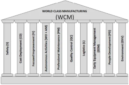
World Class Manufacturing (WCM) is a structured and integrated production system that embraces all plant processes, from safety to the environment, from maintenance to logistics and quality. The aim is a continuous improvement production performance, through a progressive elimination of waste, so as to guarantee product quality and maximum flexibility in responding to customer requests, through the involvement of the people working in the plants. The areas of intervention of the WCM are divided into 10 technical and 10 managerial pillars, for each of which incremental levels of improvement are expected, with clearly identified and measurable results. [4]
2.3 The origin of WCM
The World Class Manufacturing methodology meshed up several known methods, e.g Value Management and Business Process Re-engineering aiming at reaching the excellence in processes. The main methodologies behind the WCM are:
13
• Total Productive Maintenance (TPM), methodology aimed at reducing downtimes (Zero failures);
• Just in Time (JIT) and the Lean Production, methodologies aimed at reducing stocks (Zero Stocks);
• Total Industrial Engineering (TIE), methodology oriented at reducing wastes (Zero wastes);
• Total Quality Management (TQM), methodology aimed at achieving quality at every stage of the production process and at reducing defects (Zero Defects).
• A brief description of these methodologies will be provided in a short chapter.
The paradigm of WCM production is based on the nine Zeros: • Zero customer dissatisfaction;
• Zero misalignment; • Zero bureaucracy;
• Zero shareholder dissatisfaction; • Zero wastes;
• Zero work that does not create value; • Zero failures;
• Zero lost opportunities; • Zero lost information.
14
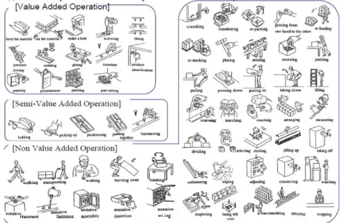
One of the important features for the purpose of the thesis is represented by Figure 2-5, where it can be seen how the displacement is considered a non-value added / semi-value added operation. This information is fundamental for the purpose of the thesis since the displacement and the relative costs are classified in this way, they can be understood as real losses for the purposes of the internal projects. They are in fact of the way that the company is forced to face in the set of transformation costs, but which can be avoided and are therefore categorized as losses.
Data gathering is carried out through the OEE (Overall Equipment Effectiveness) that is obtained as follows:
𝑂𝐸𝐸 = 𝐴𝑣𝑎𝑖𝑙𝑎𝑏𝑖𝑙𝑖𝑡𝑦 ⋅ 𝑃𝑒𝑟𝑓𝑜𝑟𝑚𝑎𝑛𝑐𝑒 ⋅ 𝑄𝑢𝑎𝑙𝑖𝑡𝑦
So the main advantages in using the OEE is to be able to “track” the performance of the plant, detailed in every single line. [5], [6]
The advantages in using the solution proposed in this document can be found in an higher performance factor and thus in an overall higher OEE.
2.4 WCM pillars
Some pillars of the WCM will be presented as they will be involved in carrying out this thesis. However it will not be the focus around which the work will be done but will determine the environment and the conditions to identify the main losses
15
that have been identified. The main aspects and the methodology will then be presented to understand the approach used in this particular type of study although the WCM methodology can be used to interpret and attack any type of loss in the establishment.
The intent is to present the 3 principally involved pillars which are: Focused Improvement, Logistics, Cost Deployment.
2.4.1 Focused Improvement
This pillar will consist using a continuous process of small improvement projects targeted at small or large areas where various tools will be used.
Focused Improvement is a technical pillar dedicated to attack major losses of Cost Deployment having a strong impact on budget and plant KPIs. FI activities are focused on solve specific problems not attackable with 7Step approach, but with the application of specific projects to find solutions and eliminate losses. A very important objective of the pillar is spreading the WCM methodology within the plant in order to reduce losses with method.
FI pillar works through the application of methods and tools provided by WCM methodology to find not only solutions but also to analyse causes that generate problems. This approach allows to restore standards with continuos improvement activities following the PDCA (Plan Do Check Act) circle as problem-solving tool.
• Plan: find the solution • Do: make a trial • Check: check results
• Act: standardize and dissemnitate knowledge Figure 2-6 Cost's prioritization
16
FI results are related to obtain savings on specific projects to reduce losses, but also to spread the WCM knowledge inside the plant, by involving people in the application of the methodology.
There are two main type of approaches, the systematic one and the focused one. Both approaches attack major losses defined with Cost Deployment. Systematic approach is related to the application of WCM 7Steps inside an area or as extention from a model area to other ones. A the beginning it is more relevant the application of WCM methodology and the use of systematic approach to spread knowledge on the shopfloor.
As all the other pillars of WCM Focused Improvement approach is based on a 7-Step methodology but there are also 7 Levels: they are a route map to apply and expand the FI activity in the plant, in terms of areas / people involved, methods and tools level, phase from reactive and preventive to proactive. They are different from 7 Steps of the pillar that explain the way to apply the pillar.
The pillar Key Performance Indicators can be resumed as follows: 1. Focused Project Benefits [k€]
2. Blue collars involvement [number of people] 3. White collars involvement [number of people] 7 Steps approach:
Step 1: Define the scope of the work. FI defines areas to attack according with the analysis made particularly by Cost Deployment with C Matrix. Other parameters can affect the choice of an area depending on priority given, like safety issues (S Matrix) and client requests for quality (QA Matrix).
Step 2: Identification of losses. To define where a plant can attack losses, it is necessary to go deeper in detail in the analysis about the definition of the smaller unit involved. The analysis consists on starting from the main plant loss, going to define its weight inside the Operative Units, Lines, till WorkStation level.
Step 3. Plan the project. Defined the area to attack, FI chooses the theme/topic more relevant inside that area, for example per type of problem or product always
17
using the Pareto approach. Focused Improvement is in charge to help other pillars to give the methodological support to apply WCM tools. Tools and Methods definition is one of the most important topic for FI pillar: they can be Basic, Intermediate or Advanced.
Step 4. Team selection. The project will be set up by selecting the necessary project team with the necessary skills requested by the type of tools used.
Step 5. Project Development. Here the PDCA approach will be implemented and used on field.
Step 6. Analyze costs and Benefits. Results need to be evaluated and B/C is calculated.
Step 7. Standardization. The solution is approved and deployed on other lines presenting the same type of problems. [7]
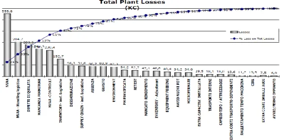
An example of the Pareto classification of the losses is presented in Figure 2-7.
2.4.2 Logistic Pillar
Logistic pillar aims at synchronizing production to market demand in order to fully satisfy the customers, to minimize inventory to create a continuous flow and to minimize the WIP and material handling. There are four main points around the solution to hit those targets:
18
1. Create conditions for continuous flow production in the plant and with suppliers.
2. Reduce significantly stocks, highlighting irregular flow. 3. Level volumes and production mix and increase saturation.
4. Minimize external transportation (e.g: direct deliveries from suppliers to the line).
5. Integrate sales, distribution, production and purchasing.
As the other pillars, also the Logistic one has an approach based on 7 Steps: Step 1: Re-engineering the line to satisfy customer. Visual stream Map are used to build a vision of the business flow that allow for a better view of the line in order to reduce the tied-up capital of the finished goods. All the activities of unpacking, picking from supermarket, kit preparation, line feeding must be moved from production to logistic operators in order to guarantee the reduction of the NVAA (Non Value Added Activities). This will results in a high level of standardization in terms of cycle time. An other target is to reduce the capital cost due to line-side stock reduction.
Step 2: Re-organize internal logistics. The activities related to this step are: • To create a pull system from assembly to warehouse
• To put in place appropriate call off systems and delivery systems in order to move the material line side to the warehouse (implementing supermarket) • To eliminate the patrolling and the forklift as handling method
• Create a cyclic feeding with high frequency of delivery in order to reduce the lineside stock.
Step 3: Re-organize the external logistics. Particular attention is paid on incoming flow and outgoing flow.
Step 4: Level the production means. Activities are resumed as: react to the demand fluctuation establishing a level of daily production. Avoid the stock peaks and manage the changeover with specific projects. The main target of step 4 is to operate with the lowest level of safety stock.
19
Step 5: Improve the internal and external logistics. Internal flows are enhanced thorough an improvement of internal call off system aiming at reducing the time of handling. One more method is to reduce the supplier distance and projects to optimize the frequency of delivery, increasing the saturation of means in order to establish a synchronization.
Step 6: Integrate sales, distribution, production and purchasing. The objective is to establish the synchronization between different functions in order to achieve the JIT in the entire supply chain. The main activities of step 6 are: purchasing involvement in the standardization during the sourcing phase, production based on lorry transportation delivery schedule and the levelling of loading customer truck.
Step 7: Adopt a sequence-time fixed scheduling method. The objective is to establish a scheduling for the daily production according to the sequence of the customer and to provide the same sequence to suppliers and pre-production in order to create a controlled flow in the entire supply chain. [8] [5]
2.4.3 Cost Deployment Pillar
The main objective of this pillar is to translate in financial costs the quantified physical losses (work-hours, kW, products). Cost Deployment is a method to establish in a rational and systematic way a program of cost reduction thorugh the collaboration between production and administration and control. The aim is to develop a plan to improve with the best methodology that can fit the problem the most relevant losses.
What is a loss? A loss is any resource (workers, materials, machines, energy) to which a cost is associated, that do not add customer-perceived value. From a productive point of view a waste is a particular losses that happen when more input resources are used with respect to those strictly necessary to produce the requested output.
Of course, also the CD pillar is developed on a seven steps approach:
Step 1. Costs perimeter definition and quantification. Transformation cost is the cost part on which WCM can act through the improvement activities.
20
Step 2. Qualitative identification of the losses. For this purpose the A-matrix is used in order to highlight the losses and the sub-processes.
Step 3: Identify the causes of the losses. Matrix B of the system is used to relate the losses with their category. The goal is to identify the cause (e.g: breakdowns) and the effect (extraordinary maintenance) relationships.
Step 4: Losses quantification. For this purpose the C matrix is used to identify losses in financial terms, relying on the effective cost of the plant. The C-Matrix highlights the costs coming from causal losses of the processes and so the losses leading to major costs, using a Pareto graph.
Step 5: Methods identification to save losses. Again a matrix is used, the D-Matrix. This tool is used to identify the methodologies and the knowhow necessary for assigning to pillars the responsibility and the priority with respect to the single losses.
Step 6: Estimate the benefit/costs ratio and identify a project team. The goal is to present a priority on a cost basis and to measure projects with respect to objectives and PDCA. Different type of saving are classified as follows:
• Hard saving: effective costs reduction with benefits in terms of workers, scraps, energy and so on.
• Virtual saving: this type of saving is explained with an example. The benefit of the improvement activity is not visible because for example an NVAA reduction has been carried out on a station that is not the bottleneck. This lead to a saving that is not “visible”.
• Soft Saving: It’s a benefit relying on a real saving that can be guaranteed during the production period. Working in a proactive way during the design phase losses can be minimized.
• Cost avoidance: it’s a cost incurred in order to avoid a greater loss. The preventive maintenance is a cost avoidance activity.
Step 7: implementation of improvement plan. The F Matrix allows to keep under control the progress of projects month by month, realizing the benefits obtained. The goal is to establish an improvement plan and to manage its progress. [9]
21
3 State of the Art
3.1 Input Data Analysis
The state of the art for data analysis is to be found, obviously in statistics. There are several methods present in the literature for data analysis. In particular, when the object of the study is a series of data which has to be attributed to a certain statistical distribution, there are different methodologies and tests that can be used. The interest is oriented at modelling a sequence of times according to a known distribution that can then be used to construct a behavioural model of the system. To do this there are several methods that provide information on the degree of similarity of the data to a known probability distribution function. It can’t be said that data in question follow a known distribution even when analyzing a sample generated ad hoc. It can in fact be asserted, depending on the test results, a degree of "similarity" of the data to the distributions that tests are trying assign to it based on the information found, and then decide whether to accept or not the risk that these do not belong instead to that given distribution. The techniques used for the case in question will therefore be briefly illustrated with the main statistical tools most used for this type of analysis.
3.1.1 Chi-squared test
A chi-squared test, also written as χ2 test, is any statistical hypothesis test where the sampling distribution of the test statistic is a chi-squared distribution when the null hypothesis is true. Without other qualification, 'chi-squared test' often is used as short for Pearson's chi-squared test. The chi-squared test is used to determine whether there is a significant difference between the expected frequencies and the observed frequencies in one or more categories.
In the standard applications of this test, the observations are classified into mutually exclusive classes, and there is some theory, or say null hypothesis, which gives the probability that any observation falls into the corresponding class. The purpose of the test is to evaluate how likely the observations that are made would be, assuming the null hypothesis is true.
Chi-squared tests are often constructed from a sum of squared errors, or through the sample variance. Test statistics that follow a chi-squared distribution arise
22
from an assumption of independent normally distributed data, which is valid in many cases due to the central limit theorem. A chi-squared test can be used to attempt rejection of the null hypothesis that the data are independent.
Procedure:
1. Partition the n observation into k cells.
2. Compute 𝑁i ,the observed number (frequency) of data in the 𝑖-th class
(identified by extreme points ri and li) and 𝐸i=𝑛pi , the expected frequency
of the same cell. Pi is the theoretical probability associated with class i,
under the postulated distribution:
• If the theoretical distribution is discrete, pi=p(xi)=P(X=xi)
• If the theoretical distribution is continuous, 𝑝𝑖 = ∫ 𝑓𝑥
𝑟𝑖
𝑙𝑖 (𝑥)𝑑𝑥 = 𝐹𝑥(𝑟𝑖) − 𝐹𝑥(𝑙𝑖)
3. Compute the test statistics:
𝜒02 = ∑(𝑁𝑖− 𝐸𝑖) 2
𝐸𝑖 𝑘
𝑖=1
4. Choose the significance level α of the test and find the corresponding critical value 𝜒𝛼,𝑘−𝑠−12 on the Chi-Square tables.
5. Set the test:
• H0: the random variable X conforms the postulated distribution with
parameters estimated from the input data. • H1: the random variable X does not conform.
6. The null hypothesis H0 is rejected if 𝜒02 > 𝜒𝛼,𝑘−𝑠−12 .
To set the number of the cells k, the expected frequency should higher than five observations. Since the probability for k cells correspond to 𝑝𝑖 = 1
𝑘 for each
interval, the following condition holds: 𝐸𝑖 = 𝑛𝑝𝑖 = 𝑛
𝑘> 5 → 𝑘 < 𝑛
5 . [10]
3.2 Simulation techniques
Once the behaviour of the modelled system has been defined and analysed, and the data necessary to study its behaviour are collected it remains only to decide
23
how to conduct this study. Different methodologies are possible to conduct this type of analysis, a code that replicates this behaviour could be implemented in almost all programming languages and then study the results. Optimization programs could also be used to investigate which of the many policies described above is the best in terms of performance. Another way is by discrete event simulation using software: this is the path that has been decided to follow. in fact, using simulation software, it is possible to transfer the logic model to a built-in algorithm and to obtain the quantities to be determined as outputs. These software allow to be more easily interpreted by different people and to be able to apply the different policies more immediately by changing the parameters. On the other hand, a code would be faster in performing calculations than simulation software but implementing the code would make it more laborious and more difficult to interpret by different parties. Moreover with the simulation software it is possible to control the behaviour of the system through animations that provide information on the system's real-time behaviour. Although this is not the case, some software has integrated three-dimensional models in order to carry out more advanced animations, an aspect not to be overlooked when these studies are conducted to provide managers or management with more awareness in making decisions based on the behaviour of the model. This is not the interest of the company -at the moment-, but the possibility of being able to develop animations allows people who are not practical to use software to better understand the aspects they want to highlight. The simple two-dimensional animations make it very easy to identify construction errors in the logical model, without having to wait for the end of the simulation to detect them. All these aspects make discrete event simulation more usable but in terms of performance it is more expensive in terms of computing capacity than traditional systems. Another aspect that has made the choice of the discrete event simulation preferable is that the model constructed, however articulated, should not require an excessive calculation load, especially if some measures are used to improve the efficiency of the calculation performance.
24
3.2.1 Focus on simulation
The term simulation refers to a vast choice of methods and applications that aim to mimic the behavior of real systems, usually performed on computers with appropriate software. In fact "simulation" can be a really general term from the moment when this idea can be applied in different fields, industries and applications. Nowadays simulation is more used, employed and powerful than ever thanks to the fact that computers and software are objects of continuous improvement.
Simulation, like most analytical methods, involves systems and their models. Systems are often studied to measure their performance, improve the way in which they operate or design them if they are not -yet- present (exactly the case of the study of this document). Managers and controllers of a system may also want readily interpretable help for day-to-day operations, such as helping to make decisions about actions to be implemented in a factory if, for example, an important machine stops working. It could also happen that managers who requested the construction of simulations were not really interested in the results, but in the primary objective to focus on understanding how their system worked. In fact, simulation analysts often discover that the process used to define how the system works, an action to be taken before being able to start developing the simulation model, provides really important advice on which changes may be useful. Rarely a single manager in charge of understanding how the whole system works. In fact, there are experts in machine design, material handling, processes, and so on but not in the daily operations of the system.
In this particular document the type of model that will be studied and that has been exposed in the previous paragraphs, is a logical model of the system. A model of this type is a series of approximations and assumptions (hypotheses), both structural and quantitative, of how the system behaves or how it will behave. Usually a logical model is represented in a computer program to investigate how the model behaves. If the model built behaves as the real system, the objective is to get more information on the true trend of this. Since the model aims at experimenting and observing the reflection of how the real system should behave, this will not involve real resources or facilities, making simulation an inexpensive
25
tool. It is easy to have a quick answer to a large number of questions about the model and the system, by simply changing the inputs and the form provided to the program. The most advantageous part is that of being able to experiment and make mistakes on the program, where mistakes can be corrected and do not count, rather than on the real system where they do. As in many other fields, the recent spikes in the computational power of devices (and a decrease in computational cost) have led to an increase in the possibility of conducting computer analysis of logical models.
After carrying out the hypotheses and approximations necessary to evaluate the target system, it’s necessary to find a way to handle the model and analyze its behaviour. If the model is simple enough, traditional mathematical tools like queue theory, differential equations, or linear programming could be used to get the answers needed. This is an optimal situation because simple formulas could respond to the investigations and can simply be numerically evaluated; dealing with formulas (for example using partial derivatives with respect to input parameters) those could provide useful information. Even without using defined formulas, an algorithm could be developed to generate numerical answers to the system under analysis, but there would still be precise answers rather than estimates subject to variability and uncertainty. However, as the present case, many systems which need to be idealized, so to be studied, are rather complicated to be modelled through simple formulas, or they require proportionally difficult algorithms such as the system. For these models that may are not perfect mathematical solutions, those are the cases in which simulation is preferred.
3.2.2 Method selection
In fact, simulation is the method used to model the system, as the policies that guide it and consequently the output variables are complicated to model through simple formulas. In fact, extremely important parts for evaluating the performance of the system are the waiting times for transport, which in turn depend on the position of the vehicle itself. Also the total crossing time of the products is a function of both the positions of the AGV and its state of use, as well as its use depends on the number of trolleys that want to be transported. Also the possibility
26
of interrupting the AGV run if this were to use advanced software would depend on the point reached by the vehicle and whether this should have passed or not the node from which the transport request are released. Building these dynamics in a mathematical way using formulas or with an algorithmic method would indeed be very complicated, as well as managing policy changes to appreciate the resulting output changes. These difficulties, combined with a more versatile use of simulation software, make it preferable to use the latter also to help understand the behavior of the model, which, if presented with pure equations, would be difficult to understand for those people who have not developed it or do not know the methods.
As stated in [11]:
“Conventional approaches used in modelling manufacturing systems can be divided into two types: Analytical models and simulation models. Both technique defines the system as mathematical equations and it can optimize the system. However, since modelling a system as mathematical equations requires a lot of assumptions about the system and the more assumptions are considered the more the system becomes unreal. On the other hand, simulation technique may not give optimal solutions. It investigates a system’s long-term behaviour. In spite of the fact that generating a solution about a system is more time-consuming in simulation technique, it is more convenient in modelling complex systems than analytical technique.”
3.2.3 Computer Simulation
The term “computer simulation” refers to the methods to study a great variety of models of real world systems through numerical evaluation using software in order to imitate the operations or features of the system, often in the long term. From a practical point of view, simulation is the process to define and create a computer model of a real or proposed system with the aim of carrying out numerical experiments to provide a better understanding of the behavior of that system under a set of hypotheses and given conditions. Although nothing prevents from using it to study simple systems, the real advantage is to use this technique to evaluate and study more complex systems. It must be pointed out
27
that simulation is not the only tool with which to study the system, but it is often the method chosen. This is due to the fact that the simulation model could become more complex as the precision associated to the model look like the real system increases; and despite this complexity it could still be used simulation analysis. In fact, the model used in this document was created with the intent to carry out a first analysis to move towards a right direction, before implementing decisions from which it is impossible to go back. The model object of the study could also be seen as a starting point from which it is possible to evaluate other alternatives in a fairly simple way. Other methods may require hypotheses too simplifying to approximate the system and allow its analysis, action that could invalidate the validity of the model under analysis.
The reason why the simulation has become so widely used is its ability to manage very complicated models corresponding to equally articulated systems. This is what makes the simulation a versatile and powerful tool. Another reason for the increasing spread of the use of these methods is also the improvement of the performance / price ratio of computer hardware, making it cheaper what was excessively expensive from a computing point of view. Furthermore, advances in the power of simulation software, flexibility, and ease of use have made it easier to move from low-level programming methods to newer, faster and more valid ones in decision-making.
3.2.4 Important aspects
However, particular attention must be paid because many real systems are subjected to different uncontrollable and randomic inputs, so their simulation models involve random or "stochastic" components which generate random outputs. These sources of randomness propagate within the logic of the model causing for example cycle times and random throughput as well. Doing just one run of a stochastic simulation is like running a physical experiment only once: probably doing it a second time, you will probably see something different. In many simulations using a longer time horizon the results trend will prove to be more stable but it will be difficult to determine the duration to be considered long enough. Furthermore, the model could be interrupted by a particular condition (as will be the object of our study). Therefore attention must be paid to the design
28
and analysis of the simulation experiment to take into account the uncertainty of the results, especially if the simulation time horizon is relatively short. Even if the output of the simulation is uncertain the uncertainty can be managed and even reduced through simplifying hypotheses. However, care must be paid to not over-simplify the model to obtain valid and reliable results.
3.2.5 Different type of simulations
It is possible to classify the types of simulation models in different ways, but a particularly useful categorization is the following:
1. Statics vs Dynamics: a type of static simulation can be conducted on the results provided by an experiment with dice. In such a performance, time does not play an important role as it does in operational models where operations are emulated, which are instead dynamic.
2. Continuous simulations vs. discrete: In a continuous model the state of the system is free to change continuously over time. A typical example may be the level of a tank that changes with the outflow of oil. In a discrete model, on the other hand, changes can only take place in places that are specific to time, such as in a production system with the arrival or the departure of the parts to be worked, the states of the changing machines and so on. You can have both continuous and discrete elements in the same model that are therefore called mixed-continuous-discrete models. An example could be a laboratory in which constant temperature changes in the ducts cause them to break and therefore a decrease in their number. 3. Deterministic vs. Stochastic: Models that do not have random inputs are deterministic. For example, a system with a fixed calendar of events is a deterministic model. Stochastic models, on the other hand, operate with at least one random type of input, as can be the arrival of clients at a restaurant that have different service times. A model can present both random and deterministic inputs: which are of a type and which of the other depends on the level of accuracy and realism desired. [12]
29
3.3 Warm-up period
As for the analysis of the results, it is necessary to explain how these were treated. For each replica, there will be a situation consisting of a warm up time and a period where the system remains "fully operative”. The model will initially be always in a state of empty and idle when simulation starts. This is due to the fact that the model has no entity in the system and all resources, including the vehicle, are free. Since it is not possible to know the necessary duration to bring the system up to a steady state, and guessing it may lead to evaluation’s errors, it is also difficult to determine the total duration of the simulation. The final estimate of performances could be biased from the first period in which the state of the system was under or over estimated.
Even if it is not possible and not convenient to guess it before running the model, one solution may be to fill the system with a finite number of entity. It is not a good solution since no methods are available to identify how many entities to place in buffers, and
after all, this is one of the question the simulation is supposed to answer. In Figure 3-1, a general representation of a performance’s phases is presented.
Other solutions are available such as running the model for a very long time so that the initial bias would be overhelmed by the other data. This may be effective in models where the biasing effects of the initial conditions wear off quickly. However, another method is to get the model going and let it "warm up" to the point where the effects of the initial conditions have vanished. Once reached this point the statistical estimators can start, accumulating statistics from then on. By doing this, the system state would not start on an idle and free state.
30
3.3.1 Welch Method
To identify the warm up period, different methods can be used, one of which is the Welch method. This is a qualitative method, intuitive subjective and quite easy to use.
1. Run n>5 replications and collect Yij measures (replication I, measure j).
2. Calculate the average of each sample j using i replicaitons.
Where: 𝑌𝑗 = ∑ 𝑌𝑖𝑗
𝑛 𝑖=1
𝑛
3. Trace the mobile average with windowing through w samples (where w<=𝑚 4 ) 𝑌𝑗(𝑤) = { 1 2𝑤 + 1 ∑ 𝑌𝑗+𝑘 𝑤 𝑘=−𝑤 𝑤 + 1 ≤ 𝑗 ≤ 𝑚 − 𝑤 1 2𝑗 − 1 ∑ 𝑌𝑗+𝑘 𝑗−1 𝑘=−𝑗+1 1 ≤ 𝑗 ≤ 𝑤
4. Select d to be the value after which the mobile average seems to be converged. Measure 1 2 3 . . m Replication 1 Y11 Y12 Y13 -- -- Y1m 2 Y21 Y22 Y23 -- -- -- 3 Y31 Y32 Y33 -- -- -- . -- -- -- -- -- -- . -- -- -- -- -- -- n Yn1 -- -- -- -- Ynm Y1 Y2 Y3 Ym
31
3.4 Notations and methods
The following notation will be used to conducts the output analysis: • n: is the number of replications.
• Y: performance estimated through simulation.
• Yi: Performance measured from replication i (i=1, … ,n)
The mean is calculated by:
𝜇̂ = 𝑌̅ = 1 𝑛∑ 𝑌𝑖
𝑛
𝑖=1
Sample variance of the measure Y:
𝜎̂2 = 𝑆2 = ∑ (𝑌𝑖 − 𝑌̅)
𝑛 𝑖−1
𝑛 − 1 The variance of the sample mean:
𝑉𝑎𝑟[𝑌̅] = 𝑉𝑎𝑟 [∑ 𝑌𝑖 𝑛 𝑖=1 𝑛 ] = 1 𝑛2𝑉𝑎𝑟 [∑ 𝑌𝑖 𝑛 𝑖=1 ] = 1 𝑛2∑ 𝑉𝑎𝑟[𝑌𝑖] = 1 𝑛2 𝑛 𝜎2 = 𝑛 𝑖=1 𝜎2 𝑛 Thus replacing 𝜎2 with 𝑆2:
𝑉𝑎𝑟[𝑌̅] = ∑ (𝑌𝑖 − 𝑌̅)
2 𝑛
𝑖=1
𝑛(𝑛 − 1) And the t-statistic is:
𝑡 = 𝜇̂ − 𝜇 𝜎̂(𝜇̂) =
𝑌̅ − 𝐸[𝑌] 𝑆/√𝑛 From the statistic:
𝑌̅ − 𝜇
𝑆/√𝑛 ≈ 𝑡𝑛−1 The probability to stay in a given interval:
𝑃 (𝑌̅ − 𝑡𝑛−1,1−𝛼 2 √𝑆2 𝑛 ≤ 𝜇 ≤ 𝑌̅ + 𝑡𝑛−1,1−𝛼2√ 𝑆2 𝑛 ) = 1 − 𝛼
32 Where 𝑡𝑓,1−𝛼
2
is the 100 (𝛼
2) % percentile of the t-distribution with f degrees of
freedom. Thus the interval estimation is:
𝑐 = 𝑡𝑛−1,1−𝛼 2
√𝑆2 𝑛
Where 𝛼, the significance level at which the confidence interval has been calculated, set to 5%. The t-interval is wider than the interval built with normalized distribution, so if data are not normally distributed the t-interval is approximated. If data were not normally distributed, the t statistic used for the test would be approximately be t-distributed for the Central Limit Theorem and thanks to a large amount of data. [10]
For evaluating the confidence interval, when more than one performance is estimated from the same experiment, a global type I error needs to be considered. In the construction of the confidence intervals an 𝛼 = 2% has been used.
Denoting with Is the 1 − 𝛼𝑠 the confidence interval of 𝜇𝑠 (with 𝑠 = 1, 2, … , 𝑘), the
probability that all the confidence intervals contain their respective true measures is equal to:
𝑃(𝜇𝑠 ∈ 𝐼𝑠, ∀ 𝑠 = 1, 2, … , 𝑘) ≥ 1 − 𝛼𝑠
3.5 Bonferroni approach
For the purpose of comparison the Bonferroni approach will be used. It rely on the hypothesis that one of the scenario is a “standard”.
• The standard variant is named 1 and the other 2,3, … ,k.
• This procedure aims at building k-1 confidence interval for the differences: 𝜇2− 𝜇1 , 𝜇3− 𝜇1 , … , 𝜇𝑘− 𝜇1 with an overall CI 1 − 𝛼.
• Each individual confidence interval is constructed at level 1−𝛼
(𝑘−1) .
33 𝜇𝑖 − 𝜇1 ∈ 𝑌̅ − 𝑌𝑖 ̅ ± 𝑡1 1−𝛼 2,𝑣 √𝑆𝑖2 𝑏 + 𝑆12 𝑏 𝑣 =(𝑏 − 1)(𝑆𝑖 2+ 𝑆 12)2 (𝑆𝑖2)2+ (𝑆 12)2
Being b the number of observation.
For the analysis an overall 𝛼 = 1% will be used. [10]
3.6 Subset selection
This procedure aims at selecting a subset of systems that includes the best choice, it delivers a set of feasible scenarios I⊆ {x1, x2,, . . . , xk} with a guarantee that
𝑃 (𝑥𝐵∈ 𝐼) ≥ 1 − 𝛼 1. Given 𝑛𝑖 ≥ 2 observation from scenario xi, set
𝑡𝑖 = 𝑡 (1−𝛼) 1 𝐾−1,𝑛𝑖−1 The (1 − 𝛼) 1
𝐾−1 quantile of the t-distribution with 𝑛𝑖 − 1 degrees of freedom
for 𝑖 = 1,2, … , 𝐾.
2. Calculate the sample mean and the sample variance 𝑆2(𝑥 𝑖) = 1 𝑛−1∑ (𝑌𝑗(𝑥𝑖) − 𝑌̅(𝑥𝑖; 𝑛𝑖)) 2 𝑛𝑖 𝑗=1
for i=1,2, …, k and the threshold: 𝑊𝑖ℎ = ( 𝑡𝑖2𝑆 2(𝑥 𝑖) 𝑛𝑖 + 𝑡ℎ 2𝑆2(𝑥ℎ) 𝑛ℎ ) 1 2
3. Form the subset
35
4 Problem Statements
4.1 Process description
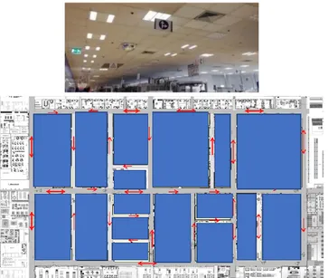
To facilitate understanding of the phenomenon under study, the behaviour of the system will be illustrated schematically. In fact, the phenomenon to consider is the materials handling between one line and the next; this operation is currently carried out by human operators, they take the carts and bring them to the next stations walking in the plant. This operation is required to let the processing phase of the downstream process takes place.
The first and second lines (which are surface moulding technology) are not lines dedicated exclusively to the product under study. In fact, the first line has a production capacity that is almost twice the capacity of the Back-End line. The three lines, where the processing of the product takes place, are scheduled to the production of this ECU for a different number of shifts during the course of the week.
The plant contains several SMT (surface moulding technology) lines; however, when the production line of a product is changed, it must be “validated”. This feature is necessary for industrialization issues and often is requested by the customer; this implies that, in addition to the cost of validation, the SMT lines associated to the products are moved only in extreme cases or to face extraordinary scenarios that may involve the launch of new products or particularly serious faults. A further constraint is given by complications related to the components that will be used to populate the boards: those must be inserted in the lines with dedicated instruments (Feeder of Reels) that serve to feed the Pick & place machines present on the lines. Furthermore, a logistic change is involved because these components are supplied through autonomous driving vehicles (AGV) which are programmed. A shift in production lines is therefore allowed but subject to several constraints which therefore requires the involvement of several figures, careful control and planning to coordinate all the necessary operations.
At the end of the first phase the products are placed in the racks, each of which can contain a total of 25 cards. The racks are then placed in the cart: it can carry
36
4 racks simultaneously for a total of one hundred motherboards (two hundred products). On the line there are up to 12 trolleys, capable of meeting production needs at times when product requirements are particularly high. From an Engineering point of view the high number of carts on the line to store the products act as dampers of variability as far as the production capacity is concerned. This guarantee that the first line is never in the condition of blocking, and at the same time to the second line of never being in a state of starving. The populated PCBs then arrive in groups of one hundred ordered in the carts, where then in the second phase of the process the racks are prepared in the loading station which has the function of extracting the individual cards from their seats and then inserting them in the processing line. As mentioned before, within the second line, in the second phase of the processing, the electronic components are picked up by the reels to populate the second side of the PCBs and the connectors are added in a line station. Since each card will then be divided, two connectors are mounted on each product, one for each product that will be obtained. However, these devices are much more voluminous and reduce the number of products that can be allocated in the racks, bringing the maximum number of products per rack to less than half compared to those that could be previously allocated. In fact, if before each rack could hold twenty-five cards, now the maximum number is reduced to ten products per rack. Each trolley containing the products leaving the second line therefore carries four racks for a total of forty cards carried, against the hundred of the previous ones.
For the purposes of the study case it is very important to evaluate this phenomenon in which a redistribution of products takes place in the carts; the displacement action performed by the operators ceases to exist, when, on the third line, the finished products are taken from a shuttle by a logistics operator. He picks up the finished products that have been packed on the line and, by
37
means of a towing, hook up to the warehouse the load. The production process can then be considered completed and the products will be stored in the warehouse or, preferably, shipped immediately.
To provide a rough estimate of the time needed for the displacements, consider a batch of four hundred pieces in which the movements are made by hand by the operators. These four hundred pieces were originally therefore two hundred cards that require a displacement of two carriages from the first to the second line, and of five carriages from the second line to the Back-end. In total there are seven sections that at best (no interference and a displacement speed of about 1.9 meters per second moving the cart) lead to considerable labor losses, considering that operators should subsequently return to the line from which it comes.
These costs are calculated as follows:
• Batch constituted of four hundred pieces, and therefore two hundred cards. • The carts brought from the first line to the second are therefore two.
• The trolleys carried from the second line to the final line are therefore five. • Distance from first line to second line: 140 meters.
• Distance from second line to Back-End: 130 meters.
The distances must be traveled twice, the outward when the operator brings the cart full and then to the return when he brings instead an empty cart.
Identifying with D12 the total distance to be covered between the first and second
line and with D23 the distance to be covered between the second the Back-end is
therefore:
𝐷12 = 140 ∗ 2 ∗ 2 = 560 [𝑚] 𝐷23 = 130 ∗ 5 ∗ 2 = 1300 [𝑚] 𝐷𝑡𝑜𝑡 = 560 + 1300 = 1860 [𝑚]
The total amount of time needed to carry out the material handling operation is therefore:
38 𝑇𝑡𝑜𝑡 = 1860 [𝑚]
1.9 [𝑚/𝑠] ≅ 980 [𝑠] Therefore a total travel time for each product is calculated:
𝑇𝑡𝑜𝑡 = 980 [𝑠]
400 [𝑝𝑖𝑒𝑐𝑒𝑠] = 2.45 [𝑠/𝑝𝑖𝑒𝑐𝑒]
Considering a monthly production of about fifty thousand (50’000) products, the total time taken in a month to move this product is:
𝑇𝑡𝑜𝑡 =50000 [𝑝𝑖𝑒𝑐𝑒𝑠/𝑚𝑜𝑛𝑡ℎ] ∗ 2.45 [𝑠/𝑝𝑖𝑒𝑐𝑒]
3600 [ℎ𝑜𝑢𝑟𝑠 ] ≅ 34.03[ℎ/𝑚𝑜𝑛𝑡ℎ] since this amount of time is used by operators, it needs to be valued with an average cost of twenty-seven euros per hour obtaining the total labour losses:
𝐿𝑚𝑜𝑑 = 34.03 [ ℎ
𝑚𝑜𝑛𝑡ℎ] ∗ 27 [ €
ℎ] = 920 [€/𝑚𝑜𝑛𝑡ℎ]
These losses can be calculated on an annual basis by attributing to each month a weight of one, except for August, whose weight is considered 0.25 and December which weighs 0.75 instead.
𝐿𝑚𝑜𝑑_𝑌 = 920 [ €
𝑚𝑜𝑛𝑡ℎ] ∗ 11 [
𝑤𝑜𝑟𝑘𝑖𝑛𝑔 𝑚𝑜𝑛𝑡ℎ𝑠
𝑌𝑒𝑎𝑟 ] = 10120 [€/𝑦𝑒𝑎𝑟] The calculations shown relate only to the product presented, it must be taken into account that there are other products for which the processing cycle involves the handling of inter-operational material. The AGVs already present in the company serve in fact to supply the various components of the lines taking them from the warehouse and bringing them to the lines. This study wants to be the first step towards an automation of product movements starting from a sample product and from this proposing a method that can be easily repeatable and extensible to products that, like the example taken, suffer this kind of waste of labour losses. From previous chapter the time for the handling of materials falls within the category of non-value added activities (NVAA) and then should be avoided.
39
4.2 Process overview
In order to provide information about the model the real system is introduced. The aim of this paper is to evaluate different policies and dispatching rules driving the future applications; each policy has a related set of KPIs and costs.
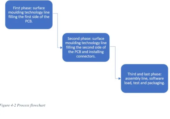
A process flowchart will be presented to identify the main phases and the hypotheses used to build the model will be explained; the details of each line will be briefly presented in order to explain how the data used as input in the simulation model were taken. The limits within which the system will be examined and then presented; a more abstract model will be used to assess the impact of decisions within the considered sub-system.
In particular, the product object of the study has been observed and it includes several sub-products: it is an engine control unit which can have different variants depending on the customer requirements. The production process is divided in three main phases carried out on different lines in the Corbetta plant.
A process macro-flowchart is provided in Figure 4-2.
40
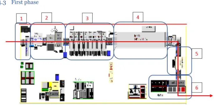
4.3 First phase
The first line is a surface moulding technology line where the printed circuit boards (PCB) are fed on a load station by an operator. Six main operations are carried out on this type of line:
1. An automatic loading machine take the PCBs and put them on a conveyor. 2. The boards are supplied with solder pastes through a silk-screen machine. 3. In this operation the first side of the board is populated through different Pick & Place machines, fed by a series of feeders for the electronic components that will then be installed on the printed circuit.
4. Once all the components have been positioned it is time to subject the product to the effect of the oven whose task is to fix the components on the board by drying the paste underneath them.
5. At this point the product is completed, through the conveyor belt it then reaches a station where visual checks are performed by an AOI (automated optical inspection) machine which judges whether the product is good or scrap.
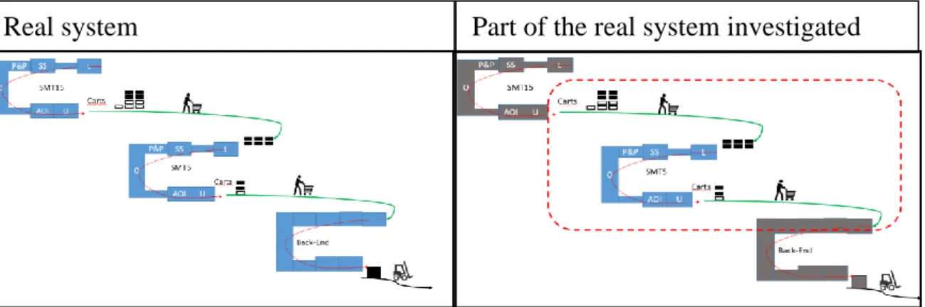
6. In the last phase the products are then unloaded and the good pieces are divided from the fail by stacking them in different racks.
After the process is finished the first side of the card is completed and the racks containing the cards are moved on carts dedicated to their movement: the Figure 4-3 Layout of the first line
41
process of the first phase can be considered finished. Operators are in charge of bringing the filled carts to the second line.
42
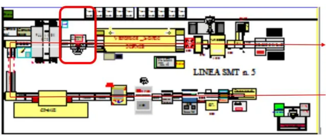
4.4 Second phase
The second phase of the process is completely similar to the first one apart for a further operation that is carried out before the products pass into the oven. In fact, a connector is also assembled to the PCBs which will be used once the products are mounted in the car. The second side is then populated, the products are again subjected to a visual inspection by the AOI machine and again the fail pieces are separated from the good ones. At the unload station they are then placed again in the racks where, however, the number of products that can be carried in the racks decreases considerably due to the fact that the connector mounted on the products makes them larger.
The second side of the board is therefore completely populated and all the hardware parts are now positioned for the control unit to function. All the products have been visually inspected by the machines, the pieces judged fail will then be inspected later; if they were to be good, they will then be put back into the process and marked as "not trouble found" NTF.
Once the racks have been placed on the carts they are ready to reach the third and final phase where the process is completed, this line is called Back End. Figure 4-4 Layout of the second line
43
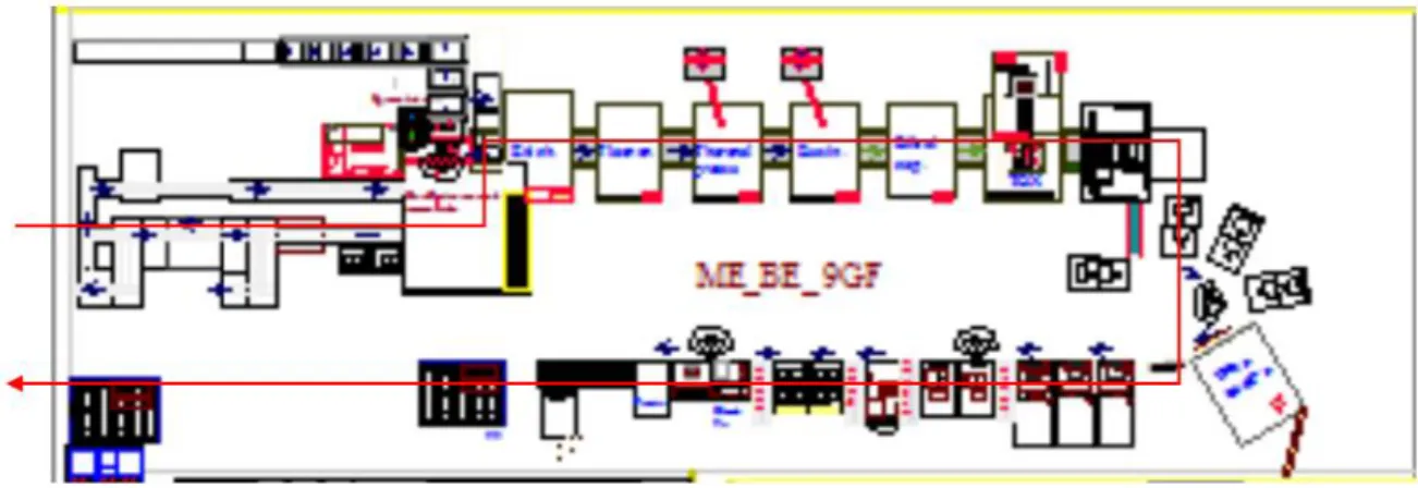
4.5 Third and last phase
The product is completed on the Back-End line where the PCB boards are separated. In fact, each individual card is made up of two pieces and in this line they are separated by a milling machine. One station is dedicated to controlling the circuit and carries out an ICT test (In Circuit Test), again the pieces judged to be fail are separated from the line by a by-pass that will allow the product to be subsequently inspected. The mechanical parts are then assembled, in particular the thermoformed cover which has the function of isolating the board and protecting its function by hermetically closing it. The piece is then tested to evaluate the hermetic seal, then followed by mechanical tests to evaluate the piece under stress and simulate the environment in which it will then have to guarantee performance in a working condition. The software is also loaded according to the versions that are being produced, and after a further test the pieces are then labelled, recorded in the logistics system. Products are packaged and ordered in boxes ready to be picked up and taken to the warehouse to be then shipped out.
4.6 Processing times
The first line, a SMT line works as described before and here summarized briefly: the printed circuit boards are fed on a load station by an operator. After that an automatic loading machine take the PCBs and put them on a conveyor, then the boards are supplied with solder pastes through a silk-screen machine, then are subjected to the action of several Pick & Place machines. Once the electronic
44
components have been placed the boards pass through an oven whose tasks is to fix the pastes. At the exit of the oven an Automatic Optical Inspection (AOI) machine carries out a visual inspection to check if components are in their correct position. The machine, after an inspection carried out on the product, records an xml file containing various information fields. Those files are used to be processed and read by software of the testing department and by the technologists, but also by the quality pillar.
The xml file is built with some fields explained here:
• Alphanumerical code corresponding to the variant of the product • The test results
• Date • Time
• Other info regarding the state of the machine
Since the output file was designed to be processed by software belonging to the testing department, whose task is to extrapolate the various types of errors reported by the machine, the xml file could not be extracted directly by Microsoft Excel.
Figure 4-6 Linear representation of the line
45
It was therefore necessary to implement a VBA code that could take multiple xml files and fill in the fields assigned. It is useful to provide technical information, which means that for each inspected product one file is created once the tests are carried out and then the products released. It was therefore possible to proceed to extrapolate the data regarding the times in which the products left the inspection machine with the related test results. Since the machine downstream of the AOI is a simple unloader of, it can be asserted that from the data obtained
there is a memory of each piece leaving the line. Therefore, taking advantage of the data obtained with this procedure, key information is provided for the purpose of modelling the system.
Since each card consists of two products, the extracted files are in fact consistent with what has been collected up to this point. In fact, the times taken from the spreadsheet report the same time two by two because they are checked together belonging to the same PCB. It is therefore immediate to collect useful data in a simple and immediate way.
For the second line the extrapolation of samples is completely similar, apart from the fact that the data relating to the products are collected in a text file that once again shows the results of the tests but above all the one that is most useful for the purposes of the studies, times. The machine on the second line is older but this allows to easily pick up the text file that can simply be backed into Microsoft Excel to perform the operations already shown for the time data related to the first line.
The analysis of the data will be shown later but to complete the information relating to the collection of these data it is necessary to better illustrate how these have been made "usable". Since the study is dealing with capital intensive lines,
Figure 4-8 Excel sheet layout