Numerical investigation of turbulent/non-turbulent interface

ALMA MATER STUDIORUM – UNIVERSITÀ DI BOLOGNA

SECONDA FACOLTÀ DI INGEGNERIA CON SEDE A CESENA

CORSO DI LAUREA MAGISTRALE IN INGEGNERIA

AEROSPAZIALE

NUMERICAL INVESTIGATION OF

TURBULENT/NON-TURBULENT

INTERFACE

Tesi in

COMPLEMENTI DI FLUIDODINAMICA LM

Relatore:

Prof. ELISABETTA DE ANGELIS

Correlatore:

Dott. ANDREA CIMARELLI

Presentata da:

GIACOMO COCCONI

Sessione III

Contents

Introduction 5

1 Turbulent/non-turbulent interface 7

1.1 An overview on the turbulence problem . . . 7

1.2 Equations of fluid mechanics . . . 9

1.2.1 Mass and momentum conservation . . . 11

1.2.2 Homogeneous isotropic turbulence . . . 12

1.3 Turbulent/non-turbulent interface . . . 16

1.3.1 The entrainment . . . 16

1.3.2 Interface detection . . . 19

1.3.3 Entrainment rate . . . 22

2 Diffusion of decaying turbulence 27 2.1 Entrainment in decaying turbulence . . . 27

2.2 Numerical simulation . . . 28

2.2.1 Set of initial conditions . . . 28

2.3 Results . . . 31

2.3.1 Flow characteristics . . . 31

2.3.2 Energy decay . . . 32

2.3.3 Enstrophy and energy scales . . . 37

2.3.4 Enstrophy balance equation . . . 42

2.3.5 Strain rates . . . 52

2.3.6 Some considerations on interface detection . . . 56

Introduction

The subject of this work is the diffusion of turbulence in a non-turbulent flow. Such phe-nomenon can be found in almost every practical case of turbulent flow: all types of shear flows (wakes, jet, boundary layers) present some boundary between turbulence and the non-turbulent surround; all transients from a laminar flow to turbulence must account for turbulent diffusion; mixing of flows often involve the injection of a turbulent solution in a non-turbulent fluid.

The mechanism of what Phillips defined as “the erosion by turbulence of the underlying

non-turbulent flow”, is called entrainment. It is usually considered to operate on two scales

with different mechanics. The small scale nibbling, which is the entrainment of fluid by viscous diffusion of turbulence, and the large scale engulfment, which entraps large vol-ume of flow to be “digested” subsequently by viscous diffusion. The exact role of each of them in the overall entrainment rate is still not well understood, as it is the interplay between these two mechanics of diffusion. It is anyway accepted that the entrainment rate scales with large properties of the flow (Tsinober 2001, Westerweel et al 2009), while is not understood how the large scale inertial behavior can affect an intrinsically viscous phenomenon as diffusion of vorticity.

In the present work we will address then the problem of turbulent diffusion through pseudo-spectral DNS simulations of the interface between a volume of decaying turbulence and quiescent flow. Such simulations will give us first hand measures of velocity, vorticity and strains fields at the interface; moreover the framework of unforced decaying turbulence will permit to study both spatial and temporal evolution of such fields.

The analysis will evidence that for this kind of flows the overall production of enstrophy , i.e. the square of vorticity ω2, is dominated near the interface by the local inertial transport of “fresh vorticity” coming from the turbulent flow. Viscous diffusion instead plays a major role in enstrophy production in the outbound of the interface, where the nibbling process is

dominant. The data from our simulation seems to confirm the theory of an inertially stirred viscous phenomenon proposed by others authors before and provides new data about the inertial diffusion of turbulence across the interface.

Chapter 1

Turbulent/non-turbulent interface

1.1

An overview on the turbulence problem

Turbulence is an omnipresent phenomenon and can be commonly experienced almost any time we are in presence of the motion of a fluid: the airflow around an airfoil, the mix-ing of air and gasoline in engines, the blood movmix-ing through the vessels, the atmospheric turbulence or the magneto-hydrodynamic flows in the earth core are few examples of phe-nomena governed by turbulence. As these examples shows, it is a subjects which affects a

huge range of science branches and engineering applications.

Since the very first days of the fluid-dynamics science, turbulence had been the main ob-stacle to a mathematical description of the motion of fluids behavior. A famous quote attributed to Heisenberg says: “When I meet God, I am going to ask him two questions:

Why relativity ? And why turbulence ? I really believe he will have an answer for the first”, Feynman defined turbulence as “"the most important unsolved problem of classical physics”, von Neumann noted in a 1949 review of turbulence that “. . . a considerable mathematical effort towards a detailed understanding of the mechanism of turbulence is called for” but that, given the analytic difficulties presented by the turbulence problem, “. . . there might be some hope to ‘break the deadlock’ by extensive, but well-planned, computational efforts.”. The study of turbulence has made progress since then but, despite

the efforts of some of the greatest minds in modern science, a full physical comprehension of many of its aspect seems still far. Perhaps the best summary of the difficulties encoun-tered dealing with turbulence is given by Kraichnan (1972): “Turbulent flow constitutes an

unusual and difficult problem of statistical mechanics, characterized by extreme statistical disequilibrium, by anomalous transport processes, by strong dynamical nonlinearity, and by perplexing interplay of chaos and order”

Turbulence, respect to a laminar flow, brings a significant increase of diffusion rates of momentum and scalar passive (hence temperature, suspended particles, solutes). A simple example can show how such rates of diffusion are incredibly greater then the molecular equivalent: if we consider the diffusion of a cigarette smoke and we hypothesize a purely molecular diffusion, the time scale of diffusion is of the order of T = L2/k (k is the

diffusivity of smoke in air). With k = ν/Sc, a Scmidth number Sc of about 0.7 for the air, a kinematic viscosity in the order of 10−5(kg/m· s) the smoke would take about 8 days to diffuse in the room, while the actual time scale thanks to turbulence is in the order of few seconds.

Some characteristic of turbulence, as the increased diffusion rates, are something desirable in some application, e.g. mixing of chemicals or heat exchangers. In some applications on the other hand, is something that must be avoided or precisely accounted for, e.g. friction reduction or ablative thermal shielding.

Should not surprise then the amount of studies that can be found on the matter, many of which are dedicated to extremely specialized and rare manifestations of turbulence. The literature on turbulence is equally vast and will be only briefly addressed further in the

reading.

The core subject of this thesis is the diffusion of turbulence when it coexist with non-turbulent fluid; despite it is a condition which can be found in almost every turbulence problem, it is still a non trivial phenomenon. For example it is accepted that the only mechanism of diffusion of turbulence in irrotational fluid is through viscous interactions, yet it seem to be Reynolds independent and it scales with big scales properties of the flow (see Townsend 1956). The literature on the subject is vast but both experimental and nu-merical analysis did until the last ten years lacked an accurate analysis on the evolution of the vorticity fields (due to technology constraints); especially the formers used to con-centrate on turbulence related quantities such the intermittency (Corrsin and Kistler 1955) which can be sometimes misleading. The recent development of PIV technology on the experimental side and the growth of computational power on the other, boosted a new wave of studies on the subject which eventually comprehended extensive study of both vorticity and strain fields (see Westerweel 2002, Liberzon 2005, Holzner 2006). In the first part of the thesis some of the results of these works will be addressed, briefly preceded by the strictly necessary theoretical framework on turbulence and turbulent interface. Will follow the results from the two different simulations carried out for this research: first the simula-tion of a an interface with decaying homogeneous isotropic turbulence without mean shear, second the study of the temporal evolution of the interface between a jet an its irrotational surround.

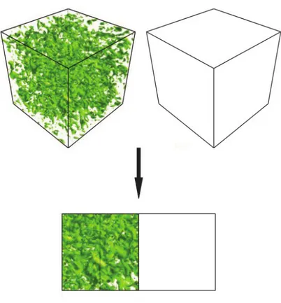
The interface with decaying turbulence can be thought as one of the most simplified cases: here a box of initially homogeneous isotropic turbulence is put beside an equivalent box of quiescent flow, a smoothing function provides the contact area between the two boxes with an initial artificial interface. The turbulence can then freely evolve and diffuse in the non-turbulent box.

The absence of any external forcing permit to reduce to the minimum the number of the parameters which can affect the interface behavior and focus exclusively on diffusion me-chanics.

1.2

Equations of fluid mechanics

In this section some basic results of fluid-dynamics will be briefly revised, these will be necessary to better understand some specific terms analyzed in this work. Furthermore it

Figure 1.1.1: Set-up of the interface experiment: a triperiodic box of homogeneous isotropic turbulence is put beside an equal box of static flow and then let freely evolve.

will show the notation used throughout the work.

The two main approaches used to describe fluids motion are the Lagrangian and the

Eule-rian representations. The Lagrangian description considers the dynamic of fluid particles,

i.e., a point which have the local velocity of fluid; thus it describes the trajectories of a specific fluid particles. The position at a given time of a particle is denoted as X+(Y, t), where Y is the position of the particle at a fixed reference time t0; Lagrangian field are in

this way indexed by the material coordinate Y. For example a velocity field is defined as

∂

∂tX

+_{(Y, t) = U(X}+_{(Y, t), t)≡ U}+_{(Y, t) (1.2.1)}

The Eulerian representation on the other hand, consider only variations of continuous fluid properties at fixed positions, through which the fluid particles moves.

The rates of change in the Lagrangian representations is usually called material or

sub-stantial derivative, which relate to the partial derivative in the Eulerian description as D Dt ≡ ∂ ∂t+ Ui ∂ ∂xi = ∂ ∂t+ U· ∇ (1.2.2)

The Eulerian representation is often preferred for its ease of use, anyway some physical aspect shown further in the reading will require a Lagrangian description. Moreover La-grangian representation is useful to investigate small scales behaviors in turbulence, as did in Holzner (2007) just to cite an example related to the thesis subject.

1.2.1

Mass and momentum conservation

∂ρ

∂t +∇ · (ρu) = 0 (1.2.3)

or

∂ρ

∂t + ρ∇ · u + u · ∇ρ = 0 (1.2.4)

in incompressible flows ρ is constant, the only other equation is then the one which grant a solenoidal velocity field or

∇ · u = 0 or ∂ui

∂xi

= 0 (1.2.5)

In this work compressibility can be safely neglected due to the low velocity and relatively low gradients experienced in the numerical experiments that will be treated.

The momentum equation relates the acceleration of the fluid particle to all the forces ap-plied to it, this lead to the Navier-Stokes equations:

∂u ∂t + (u· ∇)u = − 1 ρ∇p + f + ν∇ 2_{u (1.2.6)} or in Einstein notation ∂ui ∂t + uj ∂ui ∂xj =−1 ρ ∂p ∂xi + fi + ν ∂2_u i ∂x2 i (1.2.7) Tanks to incompressible hypothesis, taking the divergence of the last equation leads to the equation

∇2_{p =−∇ · [(u · ∇) u] (1.2.8)}

hence, for incompressible flows, pressure is not related with density and temperature by an equation of state as usual; it is uniquely determined by the velocity field. Moreover the pressure appears only through its gradient only, hence constant pressure doesn’t affect directly the momentum equation.

1.2.2

Homogeneous isotropic turbulence

For the simulation of the interface a box of homogeneous isotropic turbulence will be used as initial condition. Homogeneous turbulence means that the flow is statistically invariant to translations of the reference system, which means that the statistics of a certain flow property are the same in any point of the domain (there are no spatial gradients in any averaged quantity). Isotropy on the other hand brings invariance to rotations and reflections of the reference system, hence statistical invariance to the direction.

These simplifying assumptions mean that equation of turbulence comes without all the terms related to mean velocity fields. Furthermore it is a condition which has been ex-tensively studied and for which are available a number of consolidated theoretical and

experimental results. Kolmogorov turbulence theory provides predictions for the energy spectra of such flows and is used as starting point by many other theories. Moreover his hypothesis of local isotropy states that for large enough Reynolds numbers and for small enough regions of the space, homogeneity and isotropy are found even in non-isotropic flows.

Departures from theoretical results can be then easily attributed to the mechanics of turbulent/non-turbulent interface. While is a condition never actually encountered in real flows, a good experimental approximation of isotropic homogeneous turbulence can be obtained with grids in wind tunnels where isotropy is reached at some diameters from the grid; must noted that grid turbulence in wind-tunnels is close to homogeneity except for the persis-tence of pressure transport and transverse energy transport (see Valente and Vassilicos 2011).

In wind tunnels grid turbulence the decay of turbulence can be statistically studied prob-ing the flow at increasprob-ing distances from the grid (although this imply the use of Taylor’s frozen turbulence approximation). In homogeneous isotropic turbulence the decay of ki-netic energy can be theoretically estimated by means of the equation for the kiki-netic energy variation

∂E

∂t +∇ · (u(p + E)) = −νu · ∇ × ω (1.2.9)

or

∂E

∂t +∇ · (u (p + E) + νω × u) = −νω · ω. (1.2.10)

The flux term when averaged vanish leaving the relation for the dissipation

∂⟨E⟩ ∂t =−ϵ (1.2.11) where ϵ = 2ν ⟨ ω2 2 ⟩ (1.2.12) The former relation shows how variations in turbulent kinetic energy E, in a statistically steady flow, are balanced by viscous dissipation ϵ. Equation 1.2.12 illustrate how strictly related are dissipation and enstrophy in homogeneous isotropic turbulence.

Is useful to consider now the spectral version of the kinetic energy equation, the resolution of the Navier-Stokes equations in Fourier space will not be discussed here as it is long and can be easily found in a number of textbook. In the Fourier space for a given wave number

k, with

k = 2π

λ , (1.2.13)

(λ is the wavelength) the relation for the variation of kinetic energy becomes

∂

∂tE(k, t) = T (k, t) + F (k, t)− 2νk

2_{E(k, t),}

(1.2.14) where T (k, t) is the kinetic energy transfer due to non-linear interaction, F (k, t) is the term of forcing, and−2νk2_{E(k, t) is the dissipation.}

Now the Kolmogorov first similarity hypothesis states hat for the locally isotropic turbu-lence the energy spectrum distribution is uniquely determined by the dissipation ϵ and the viscosity ν.

The second similarity hypothesis states that, if the separation between the energy injecting scale and the dissipation scale η is large enough, in the range between these two scales (the inertial range) the energy spectrum is uniquely determined by ϵ and does not depend on ν. Starting from this last hypothesis, the dimensional analysis leads for the inertial range to a energy spectrum which decades as

E(k) = Ck· ⟨ϵ⟩

2

3 _k−53, (1.2.15)

where Ckis an universal constant.

There are a series of issues on Kolmogorov theory, first of all the validity of local isotropy assumption. A number of studies have reported some departures for high order statistics from isotropy in high Reynolds numbers shear flows (Tsinober 2001). Such flows seems to preserve in the inertial range some memory of the forcing scales meaning that the energy cascade is not an information losing process. This is only the case for flow with large scale anisotropy and high Reynolds numbers but even isotropic homogeneous turbulence seems to preserve some dependence from large scale parameters down to the dissipative range. George (1992) demonstrated the possibility of the existence of solutions to the averaged spectral equations that are both self-preserving at all scales of motion and dependent to the

initial conditions.

For decaying homogeneous isotropic turbulence, the length of validity of the similarity hypothesis is the Taylor microscale λ and the energy variation in time is related to λ by

E(t)∼ u2λ (1.2.16)

(see George 1990) and decay of the kinetic energy undergoes to a power law

u2 ∼ tn (1.2.17)

The dissipation can be related to both kinetic energy and Taylor microscale through

ϵ = 15νu

2

λ2. (1.2.18)

or either related to the integral scale through

ϵ ∼ u

′3

L =

E32

L (1.2.19)

where u′ is the r.m.s. of velocity fluctuations.

According to Von Kármán result the Taylor microscale increases as the square root of time, or λ = √ −10 n νt (1.2.20) thus dλ2 dt =− 10 n (1.2.21)

The linear growth of λ2 for decay turbulence has shown to fit with actual data in grid-induced turbulence quite well as proven for example by Comte-Bellot and Corrsin (1966). Grid turbulence has demonstrated as well a strong dependence on initial conditions of de-cay laws, Warhaft and Lumley (1978) in their study on heated grids found strong variations of temperature fluctuations decay rate depending on the initial temperature.

About the actual value of n there are multiple results depending on some characteristic of the flow. For virtually infinite initial Reynolds number the Von Kármán-Howart solution predict a decay rate of t−1, instead for finite initial Reynolds number most experiment

reports n <−1 ( Comte-Bellot and Corrsin 1971 , Wray 1998, Wang and George 2003). The power law of decay with various values for the exponent n has proven to fit well both data from grid induced turbulence and DNS but recent experiment with fractal grids ( Seud and Vassilicos 2007 and Valente and Vassilicos 2011) found the decay rate to be governed by an exponential law rather then a power law. Being

dE

dt =−10ν

E

λ2, (1.2.22)

a power law is possible only if the Taylor microscale remain constant during decay, so that the time derivative of the kinetic energy is proportional to the kinetic energy (George 2013). George and Wang (2009) shown that both decay laws are consistent with an equilibrium similarity analysis of the spectral energy equations, yet is not well understood what drives the flow to a decay law rather than the other.

1.3

Turbulent/non-turbulent interface

1.3.1

The entrainment

As mentioned in the introduction turbulence is a complex phenomenon, so some basic physical aspect of this problem must be addressed before a further insight in the subject of turbulent/non-turbulent interface.

Turbulence cover such a range of yet not understood flow behaviors that a comprehensive definition for it has not found at the time. Despite the attempts of many to found an universal definition for it, the best way to define turbulence is still by a list of its properties. Turbulent flow are expected to show:

• Intrinsic randomness in space and time variations. This feature arise form the

ex-treme sensibility to disturbance of the Navier-Stokes equations, which lead such deterministic equations to a chaotic behavior.

• An extremely wide range of scales strongly interacting together. The interaction

between the many degrees of freedom results from the non-linearity of turbulent flows.

conditions leads to much different results. Nevertheless, different realizations of the same turbulent flow shares the same statistical properties; thus turbulent flows posses both predictable an unpredictable features.

• High dissipation; turbulence require energy in order to be maintained. The energy

supply is mostly at large scales while dissipation occurs at small ones.

• Three-dimensions and rotational field, even if there’s still a debate about the

exis-tence of 2D turbulence.

• Strong diffusion; transport processes of momentum and passive objects are enhanced.

Aside the qualitative definition of turbulence there are some quantitative features which can be used in order to identify the onset of turbulence (e.g. vorticity thresholds), though such features depends on the flow characteristics and lacks the universality of the afore-mentioned definition. Some of these quantitative features will be shown further in the work as will arise the need for a detection algorithm of the turbulent interface.

In most bounded flows and in all practical cases of unbounded flows, turbulence coexists with regions of irrotational flow: boundary layers, jet, wakes, plumes, mixing layers (ba-sically all the free shear turbulence) are examples that show how vast is this category of phenomena. The interface between the turbulent flow and the surrounding inviscid irrota-tional flow appears highly irregular and convoluted, its shape and position ever changing. The first attempt of dealing with such physical problem has been through the definition of the intermittency γ (Corrsin and Kistler 1955), which is the fraction of time in which a fixed point of measurement experience a turbulent flow. Such ratio has been derived directly from the first hot-wire velocity measurement in the regions at the boundaries of turbulent flows, where the probes experience strong fluctuations for small time intervals. With a process called entrainment non-turbulent fluid, due to the action of neighboring rotational flow, acquires vorticity, and become part of the turbulent mass; thus the region affected by turbulence tend to spread. The onset of vorticity in irrotational flow is exclu-sively determined by viscous interactions with turbulent eddies in the interface area, there is therefore a strong relation between entrainment and dissipation.

Using the definition given by Phillips (1966) the entrainment is “the erosion by

turbu-lence of the underlying non-turbulent flow”. Entrainment is a process which concerns also

kinetic energy to it; even in the laminar case the entrainment can be related to the energy dissipation.

Entrainment has a central role in mixing properties as transport rates of momentum and vorticity as well as passive quantities like temperature or concentration of suspended phases; thus the the problem of modeling the behavior of the spreading of turbulence in an irrota-tional fluid had been at the center of many studies in the past years.

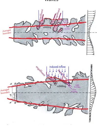
The entrainment is usually thought to act both at large and small scales with different mechanics. Viscous , i.e. small scale, interactions act diffusing into non-turbulent region and converting non-turbulent fluid in turbulent. This interactions generate small structures of rotational flow which protrude toward the irrotational fluid originating the so called nibbling.

At large scales engulfment entrap large zones of non-turbulent flow which is successively “digested” by small scale nibbling. Moreover large scale fluctuations act by increasing the surface area of the interface, thus the area affected by turbulence diffusion.

Philip classified three type of entraining flows, differentiating them on the base of the char-acteristic of their entrainment process. He stated that there are differences between grid induced turbulence, jets interfaces, wakes and boundary layers interfaces. Jet flows for ex-ample are characterized by an induced inflow of fluid which cannot be found for exex-ample in wakes and boundary layers. Hence the differences between engulfment contribute esti-mates in various studies may be probably explained by intrinsically different entrainment dynamics.

The relative weight in the entraining process of engulfing and nibbling has been at the cen-ter of many studies on turbulent incen-terfaces, nevertheless since today the incen-terplay between the two mechanism of entrainment has not permitted yet to find which is the predominant in turbulence diffusion.

1.3.2

Interface detection

The interface can defined as the thin layer across which the flow is found turbulent, i.e acquire all the properties listed the previous section. It is a convoluted unsteady surface, whit strong fluctuations of velocity and vorticity (as the idea itself of describing it through intermittency may suggests). The surface of the interface is actually hard to identify, in fact the flow in proximity of the interface is characterized by inclusions of laminar flow and bubbles of vorticity in the irrotational field which evolve continuously.

The study of partially turbulent flows pose again the problem of defining what is turbu-lence. The qualitative description given in the previous chapter can clearly discern in these kind of flows turbulent areas from the non-turbulent ones; the question is now how can be said whether a small part of the flow is turbulent or not.

A criterion to define locally when a part of the flow is turbulent must be found before proceeding in the study of turbulent interface. Most of the criteria used until now imply taking some arbitrary level of a flow quantity as marker of the inset of turbulence. Corrsin (1943) and Kistler (1954, 1955) used first the distinction in rotational turbulent region and the almost potential non-turbulent ones as discriminating criterion. Such distinction offer a quantitative mean of detecting the interface between turbulent and laminar flow but it

had been difficult to implement practically until now-days, since it requires information on vorticity.

The development of PIV permitted in the last years to measure vorticity fields in small control volumes, yet the accuracy of such measurements is poor for detection purpose and the measure of the vorticity is often used beside some other detection technique (as in Westerweel et al 2005, Holzner et al. 2006) . DNS on the other hand give access to the full velocity field data and application of a vorticity threshold as detection method confirmed itself as a valid approach; Bisset et al. (1998, 2001) as well as Holzner (2006) found a steep change in vorticity across the turbulent/non-turbulent interface.

Holzner et al (2006, 2007) gives an exhaustive analysis of a series of experimental and nu-merical interface detection techniques in a water-filled tank with grid-induced turbulence; among them is described the combined use of particle image velocimetry (PIV) and planar laser-induced fluorescence before used by Westerweel (2002). Here a fluorescent dye, with low Schmidt numbers, is injected in the turbulent part of the flow where it rapidly diffuse. The low Schmidt number ensure that the molecular diffusion is negligible respect turbulent mixing. A planar cross section of the test chamber is then illuminated by an intermittent laser sheet, two different camera capture the same image of the flow in rapid succession in such a way to obtain a normal and an illuminated caption of the flow at almost the same instant. The former caption will give the data for the PIV and the latter will show the which part of the velocity field is interested by the dye, i.e. the turbulence. With such technique the smallest scales of the dye concentration field are of the order of the Batchelor scale (Holzner et al. 2006), defined as

ηB =

η √

Sc (1.3.1)

Holzner with such method reported a smallest scale for the concentration field one order of magnitude smaller then the smallest resolved scale. This technique has also the merit to give access to the full instantaneous field of the vorticity component normal to the laser sheet plane, which has been used in order to study the enstrophy production near the in-terface. The thresholds technique have been proven before against the tracking of some passive scalar or dye (as in Westerweel et al. 2009 and Holzner et al. 2006 ), anyway both techniques tend to overestimate the position of the interface H(t) (in Holzner et al. 2006 is reported an evaluation of such errors).

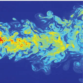
Figure 1.3.2: Concentration field of dye in turbulent jet (Westerweel 2009)

Non-rotational fluid can acquire a non-zero vorticity only by means of molecular viscous diffusion through the interface with the turbulent flow, thus the main mechanism of turbu-lent diffusion is expected to be related with small viscous scales; this is the main reason why the width of the interface across which the vorticity rise to turbulent-side’s levels is comparable to the scales of viscosity. As observed in experiments the thickness of the in-terface is of the order of the Taylor microscale (∼ Lx/Re1/2) ( Westerweel 2009), but in the absence of a strong shear the thickness may reduce to the Kolmogorov scale (∼ Lx/Re3/4) (Holzner et al. 2007, 2008). As noted before, Corrsin and Kistler (1954) used first the vor-ticity as quantitative detection technique, due to the sharpness in the separation between rotational turbulent flow and irrotational flow. Other quantities present a similar behavior across the interface, among them velocity fluctuation thresholds have been tested by both Bisset et al. (2002) and Westerweel et al. (2002). A thresholds discriminant must be im-posed due to the velocity fluctuations induced by the interface in the non-turbulent region, nevertheless these decay rapidly with the distance from the interface.

Vorticity alone is not a sufficient condition to define locally a fluid as turbulent, experi-ments must take in account for the random nature of the flow in both sides of the interface and some trace of vorticity can be found in the non-turbulent side. This virtually imply another mechanism of entrainment: weakly turbulent seeds in the irrotational part of the

flow may be entrained due to the vortex stretching mechanism as pointed out by Tsinober “ an initially Gaussian and potential velocity field with small seeding of vorticity will pro-duce - at least for a short time - an essential positive enstrophy (as well as production of strain) though strictly this is true for homogeneous turbulence” although as stated in Bisset et al. (1998, 2001) such mechanism can be effective only in the proximity of the interface where large strain should exist (fluctuations attenuate exponentially with the distance from the turbulent interface).

Beside the randomness of the flow considered above, the non turbulent side of the field is found to be subject to non-rotational velocity fluctuations induced by the movements of the interface itself. Phillips (1955) studied with a theoretical approach the energy of such fluctuations at an increasing distance ri from the interface. At sufficient distances the irrotational field can be described by a potential Φ, setting∇Φ = 0 at ri → ∞ and a random distribution of normal velocity at the interface, he predicted a decay for the average square root of the velocity fluctuation energy⟨v⟩ ∝ r_i−2. Despite the coarse assumption for the interface, the prediction had been proved to hold in a boundary layer experiment by Bradshaw (1967) yet only at several boundary layer thickness away from the interface. Recently Borrell and Jiménez questioned the capability of the threshold approach to grasp the characteristics of the interface: according to them the variation of the threshold strongly affect the topology of the interface detected and obviously its detected position.

1.3.3

Entrainment rate

As mentioned before entrainment is essentially a viscous (small scale) process, yet exper-imental evidence (Tritton 1988; Tsinober 2001; Hunt, Eames and Westerweel 2006) had shown that turbulence diffusion scale with the bigger scales of the flow. At large Reynolds number the entrainment rate and the propagation velocity of the interface (relative to the fluid flow) become independent to viscosity ( Townsend 1976, Bisset et al. 2001). Hence the overall rate of entrainment is set by large-scale parameters of the flow while the actual spreading is brought about by the viscosity (Tritton 1988). As clearly stated by Tsinober “small scales do the ’work’, but the amount of work is fixed by large scales in such a way that the outcome is independent of viscosity”. The slow diffusion of viscosity into the irrotational fluid must be accelerated by the interaction of velocity fields of eddies of all sizes, in such a way that the overall rate of entrainment is set by large scale parameters of

the flow (Holzner et al. 2007).

About the entrainment rate, two different characteristic velocity can be defined:

entrain-ment velocity uaand propagation velocity ve(as seen in Liberzon et al. 2009). The former

is the velocity of the fluid relative to the turbulent/non-turbulent interface. In their La-grangian analysis of grid-generated turbuelnce, Holzner et al. (2007) found that locally a particle cross the interface with a velocity which scale with the Kolmogorov velocity

uη = (ϵν)

1

4 _{, which substantially confirm the small scale nature of the onset of entrainment.}

The advancement of the mean position H (t) of the interface toward the non-turbulent re-gion gives instead the propagation velocity ve = dH/dt. Phillips (1972) related veand ua through the geometry of the interface ζ(y, z, t) (which location has been found with the threshold technique) with the equation

ve= ua ⟨

1 + (∇ζ)2⟩

1

2 _(1.3.2)

where the average refer the plane y−z. In the case of turbulence induce by a planar energy source (e.g. a vertically oscillating grid) the mean position of the interface can be predicted by the relation

H(t) =√Kt. (1.3.3)

Long (1972) theorized this relation for planar forced flows in semi-infinite spaces, anyway experimental measurements in water filled tank, accord well with theory for what concern the flow far from tank walls. The values for K have been empirically determined by regression analysis

ln(H) = n· ln(t) +1

2ln(K), (1.3.4)

the theoretical value for n is obviously 0.5, though some time slightly different values have been reported (liberzon et al. 2009, Holzner eal. 2006). The value of K depends on the fluid and, at least for water, seems to increase when certain polymers are diluted in the fluid ( Liberzon et al. 2009). Polymers seems to interfere with the classical mechanism of energy cascade and their effect on propagation of turbulence suggests that small scales interactions cannot be easily neglected in entrainment models.

that the entrainment velocity ua depends on the kinematic fluid viscosity ν and on the dissipation ϵ = 2νsijsij in the local turbulent side of the interface. Thus the entrainment velocity must scale with the dissipative characteristic velocity , i.e. the Kolmogorov ve-locity uη. This is apparently in opposition with the fact that the flux of entrained fluid is determined by big scale parameters of the flow; in Holzner et al. (2009) is proposed a the-ory which can conciliate the small scale entrainment mechanism with the big scale rate of entrainment. They argue that the global entrainment flux, i.e. Q = veA0, occurs through a

large scale (or projected) interface area A0, and the strongly convoluted total interface area Aη adjust itself to account for the same flux with a much smaller characteristic velocity so that

Q = veA0 = uaAη ∝ uηAη, (1.3.5)

although they have not been able to find how the total area should adjust itself in such way. This hypothesis relates then the big scales with the small ones through the entrainment flux, according to this the ratio between the two areas is

Aη A0 ∼ ve uη (1.3.6) being uη ∼ ν/η , we have Aη A0 ∼ veη ν . (1.3.7)

Sreenivasan in his study on fractal dimensions of turbulence (Sreenivasan et al. 1989) found that Aη A0 ∼(η L )2−d (1.3.8) where the value found for d is 7/3. We can now write the propagation velocity veas

ve ∼ ν ( L η4 )1 3 = ν η ( L η )1 3 (1.3.9) which show how the propagation velocity scales with the ratio between the greatest scale in the field and the dissipative length.

ve ∼

ν

ηRe

1/4

L (1.3.10)

Must be said that at the present there is only indirect evidence for the assumption that

ua ∼ uη, no precise measurements of the local velocity of the interface are available at the present day. Since now the experiments performed in order to measure the behavior of the interface relied on PIV measurement which can extract only one vorticity component of the field with significant errors in the non-turbulent side of the interface (see for an assessment of the measurement error Westerweel et al. 2009). Holzner et al. (2009) addressed the problem with a numerical experiment of grid turbulence, they observed that the iso-surface of enstrophy (constant ω2) evolve according to

∂ω2

∂t + uj

∂ω2 ∂xj

=−ua|∇ω2|. (1.3.11)

The enstrophy balance equation on the other hand gives 1 2 ∂ω2 ∂t + 1 2uj ∂ω2 ∂xj = ωiωjsij + νωi∇2ωi, (1.3.12) from equation 1.3.11 and 2.3.22 we can obtain an equation for uacomposed by an inviscid and a viscous contribution

ua=−

ωiωjsij

|∇ω2| −

νωi∇2ωi

|∇ω2| . (1.3.13)

In their simulation Holzner et al. found a uaabout two time smaller than uη, moreover they found that locally the viscous term strongly prevails over the inviscid interaction strain-enstrophy.

A note must be done about the range of validity of the aforementioned theories, all the data and the studies available at the present day involve modest Reynolds numbers, the usual Re goes from 103 _{for wakes and jets (e.g. Westerweel et al., Mathew et al., Khashehchi et al.)}

experiments to few decades for some grid induced turbulence (Holzner et al. , Liberzon et al.). At the much higher Reynolds number usually encountered in applicative fields, the behavior of the interface has not been yet extensively studied, due to the limitations of both measurement instruments and computational simulations.

Chapter 2

Diffusion of decaying turbulence

2.1

Entrainment in decaying turbulence

The simplest model of a turbulent flow is the case of homogeneous isotropic turbulence.Such flow does not find any equivalence in a real experiment, though some flows like grid gen-erated turbulence tend to the homogeneous isotropic behavior; yet it is an useful starting point for the comprehension of turbulence mechanics since it possesses certain character-istics shared by all commonly studied turbulent flows. Homogeneity of the flow means statistical invariance of flow quantities with respect to translation in any direction, whereas the isotropy assumption brings statistical invariance with respect to rotations and reflec-tions of the coordinate system.

In this investigation we started then creating a field of homogeneous isotropic turbulence, from such field we generated the initial conditions for the interface simulation then we sim-ulated the diffusion of the decaying turbulence in such domain. The present work of thesis belongs to a more general research project aiming at studying the turbulent/non-turbulent interface. Here we start with the analysis of the turbulent/non-turbulent interface with de-caying turbulence. The results obtained will be used then as starting point for the study of turbulent/non-turbulent interface with forced turbulence. The parameters of the simu-lation are hence intended to match the parameters of previous experiments with shearless interfaces in water filled tank (Holzner et al. 2006, Liberzon et al. 2009). The simula-tion of unforced, freely evolving turbulence differs in many aspect from such experiments, nevertheless has shown to share many aspect in interface behavior with them.

2.2

Numerical simulation

For both the generation of the initial turbulent field and the simulation of the decaying tur-bulent flow, a pseudo-spectral DNS code has been used. Pseudo-spectral codes solve the partial differential equation system generated by Navier-Stokes equations in the Fourier space. To keep the code efficient non-linear terms are transformed back to the physi-cal space and there estimated; this operation has a computational cost of the order of

O(N log N) (thanks to fast Fourier transform algorithms) while the estimation via

con-volution of the non linear terms in the Fourier space require O(N2)operations, thus the choice for the former.It is to note that Pseudo-spectral codes have the important feature of the spectral accuracy property. The code utilized in the present work has already been used in previous works on homogeneous isotropic turbulence (De Angelis et al. 2005).

2.2.1

Set of initial conditions

As starting point a cubic domain of homogeneous isotropic turbulence had been created. All the initial conditions for the interface simulations in the present work have been origi-nated from a unique run of a 128× 128 × 128 grid points domain.

The equation of fluid motion in the Fourier space used in the present work is

∂ ˆu

∂t = ˆH− νk

2_ˆ

u + ˆF, (2.2.1) where ˆH and ˆF are terms respectively associated to the non linear and the forcing term

through ˆ H = ˆh− k k2(ˆk· ˆh) (2.2.2) ˆ F = ˆf − k k2(ˆk· ˆf). (2.2.3)

The terms ˆf and ˆh are respectively the Fourier coefficient of forcing term and of the non

linear term

hi =−uj

∂ui

∂xj

The forcing term has the goal to force on a limited band-width around a given wave number k2 k2 = √ k2 x+ k2y+ kz2 (2.2.5) k2_min ≤ k2 ≤ k2_max, (2.2.6) with a random amplitude which follow a Gaussian distribution over the assigned wave numbers range. ˆ fi(kx, ky, kz, t) = ˆf0· e σ −1 2( √ k2−µ2 σ ) 2 (2.2.7) The range chosen is 3.2≤ k2 _{≤ 6.8 around the wave numbers with µ}2 _{= 5 and σ = 6.}

The total temporal length of the simulation has been of about 72 integral time scales t0.

t0 =

L0

urms

(2.2.8) After the statistical stationarity has been reached, 25 independent initial fields have been selected.

The Reynolds number has been computed as

Reλ =

urms· λ

ν , (2.2.9)

and the Taylor microscale λ has been computed as

λ = √ 5· urms ⟨ω2⟩ (2.2.10) ner_{of fields N} x× Ny× Nz Lx,Ly,Lz Re Reλ λ η ∆t t0 25 128× 128 × 128 2π 120 52 0.242 0.017 0.001 0.23

Table 2.1: Initial fields parameters

In order to simulate the interface, a field composed by two neighboring identical velocity fields of 128× 128 × 128 points has been created; due to the periodic boundary condi-tions, the interface between the two fields this does not generate discontinuities of any

sort. The new initial velocity field uo(x, y, z) is then multiplied by a junction function

which smoothly brings to zero the velocity field in half domain (as proposed by Tordella et al. 2008); the junction function is constructed in such a way to retain the periodicity of the field on the boundaries. The junction function is

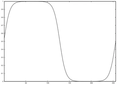
u(x, y, z) = uo(x, y, z)· p(x) (2.2.11) p(x) = 1 2 [ 1 + tanh ( a· x L ) · tanh ( a·x− L/2 L ) tanh ( a· x− L L )] (2.2.12)

Here the constant a is a parameter which affects the initial width of the interface and L is the domain length. For the current simulations the parameter a has been set at 6π, the values have been chosen in order to grant an initial thickness large enough to be resolved.

0 0.1 0.2 0.3 0.4 0.5 0.6 0.7 0.8 0.9 1 50 100 150 200 250

Figure 2.2.1: The smoothing function p(x) for the initial interface

The fields generated is such way have been then let freely evolve for 2000 time steps ∆t ( or 10 integral time scales), the turbulence in them spreading and decaying. The result is a series of velocity field constituted by a center core of approximatively homogeneous isotropic turbulence, while the field become more and more anisotropic closer to the in-terface. As can be seen in the figure each field consist of two interfaces thus a total of 50 interfaces over 20 time intervals each constitute the data-set we have used for our study.

The spatial resolution , i.e. the smallest structure that can be resolved is given by smallest wave number of the field, namely

kmin =

2π

128 = 0.049. (2.2.13)

2.3

Results

From each of the 25 initial condition we have started an independent integration without forcing. From each of those 20 fields have been saved at regular time intervals, for a total of 500 fields and 1000 interfaces. Anyway only about half of these have been taken in account for the following results, precisely only all the temporal step greater then it=1200 constitute the data set for the analysis. Such reduction has been necessary in order to exclude transitory phenomena and let the flow to lose every memory of the artificious initial interface. Almost all results in the present work are spatially averaged in planes normal to the direction of diffusion, i.e. the coordinate x. These statistic in each plan have been then ensemble averaged with its symmetric counterpart respect the centerline of the turbulent part of the flow; finally the results have been ensemble averaged over all the 25 fields. Thus the statistics that will be presented in this chapter come from the evaluation of 819.000 points for each plane y− z and each time interval, number which has shown large enough for the convergence of the statistics.

2.3.1

Flow characteristics

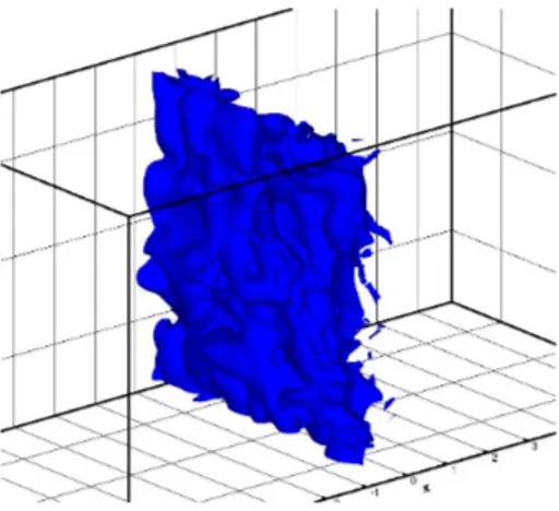
The flow obtained from our simulation is constituted by a core of almost homogeneous isotropic turbulence which spreads and decay in an irrotational fluid. Due to the imposition of periodic condition, at every boundary the flow is imposed to be the same on opposite sides of the domain box, hence the two apparently separate interfaces actually propagate from the same turbulent core. The diffusion of turbulence from this core is continuously counteracted by the dissipation in such a way that the turbulence cannot fill the field, and the two interfaces never come in contact in the temporal range of the simulation. For the purpose of the present work two sections of the turbulent flow are of particular interest: the center plane of the turbulent flow and the average position of the initial interface (x=0), which will be indicated hereafter simply as turbulent core and interface, respectively. The

Figure 2.3.1: Iso-surfaces of kinetic energy: 10% threshold.

former is useful to show the differences in decay rates and other flow properties respect the ideal case of homogeneous isotropic turbulence; the latter instead is indicative of the flow evolution in the volume of flow affected by the interface.

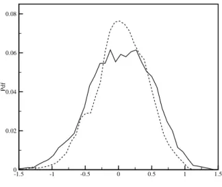
The interface region nevertheless change sensibly in its shape with time, ever producing new turbulent structures, bubbles of vorticity and engulfing pockets of laminar flow. As can be seen from the probability density functions of the longitudinal velocity fluctu-ations (figures 2.3.2 2.3.3), the field is strongly intermittent in proximity of the interface and negatively skewed; on the other hand field in the turbulent core shows an almost sym-metrical distribution and a more regular profile.

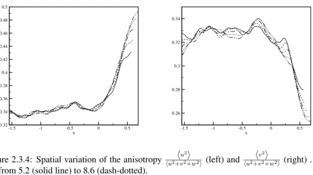
The anisotropy levels, defined as

⟨u2

i⟩

⟨u2⟩ + ⟨v2⟩ + ⟨w2⟩, (2.3.1)

indicates that the relative weight of velocity fluctuations in the longitudinal direction slowly grows in the turbulent interface, in correspondence of which it start to peaks fast. The eval-uation of the anisotropy is truncated at the beginning of the laminar side where the ratio is biased by the numerical noise.

2.3.2

Energy decay

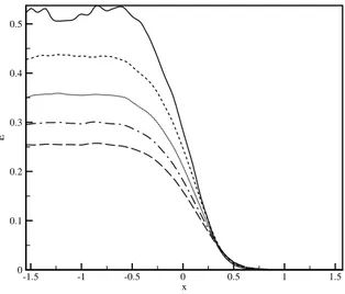
The average kinetic energy of the field results to be a function of both time and x coordi-nate. The profiles shown in figure 2.3.5 evidence such dependence: at a given time, the

P d f -1.5 -1 -0.5 0 0.5 1 1.5 0 0.02 0.04 0.06 0.08

Figure 2.3.2: Pdf of u in a plane centered in the turbulent core. Solid line: t=1.8, dashed line t=2.0 P d f -1.5 -1 -0.5 0 0.5 1 1.5 0 0.02 0.04 0.06 0.08

Figure 2.3.3: Pdf of u at different positions. Dashed line: turbulent core, solid line: inter-face plane (x=0).

x -1.5 -1 -0.5 0 0.5 0.32 0.34 0.36 0.38 0.4 0.42 0.44 0.46 0.48 0.5 x -1.5 -1 -0.5 0 0.5 0.26 0.28 0.3 0.32 0.34

Figure 2.3.4: Spatial variation of the anisotropy ⟨u

2⟩

⟨u2_+v2_+w2_⟩ (left) and

⟨v2⟩

⟨u2_+v2_+w2_⟩ (right) .

t/t0from 5.2 (solid line) to 8.6 (dash-dotted).

kinetic energy keeps a flat profile until the interface is approached then it rapidly drops to zero in few Taylor microscales. The figure also shows the evolution with time of turbulent kinetic the energy: in the turbulent core of the flow it decays as expected, while a slightly increase in the velocity fluctuations can be observed in the initially non-turbulent region. The introduction of the interface brings an increase of effective dissipation with respect the case of homogeneous isotropic turbulence. In the turbulent core of the flow, where the turbulence is in first approximation still homogeneous and isotropic, the decay rate is increased due to the energy flux toward the interface. The inhomogeneity introduced by the presence of the interface produce spatial energy fluxes which tend to homogenize the flow. Hence the turbulent core release energy through such energy fluxes and experience an increased effective dissipation.

In figure 2.3.6 the normalized kinetic energy of the turbulence core and of the homoge-neous isotropic turbulence are compared. Both, after an initial evolution, follow approxi-matively a classical power law and the homogeneous isotropic has the decay of predicted by Kolmogorov theory of t−1. The turbulent flow with the interface shows instead a larger decay rate of t−75 , which is mainly due to the energy flux toward the interface. Hence the

interface act as a sink of energy for the turbulent core.

x E -1.5 -1 -0.5 0 0.5 1 1.5 0 0.1 0.2 0.3 0.4 0.5

Figure 2.3.5: Temporal evolution of the average kinetic energy in the y-z plan, solid line: t/t0 =5.2 , dashed: 6.0 , dotted: 6.9 , dash-dot: 7.8 , long dash: 8.6 (long dashed)

t/t0 E (t )/ E 0 2 4 6 8 0.2 0.4 0.6 0.8

Figure 2.3.6: Normalized kinetic energy decay of a box of homogeneous isotropic turbu-lence (triangles) and the turbulent core of the flow with the interface (squares). Solid bold:

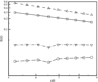
the longitudinal position x. In figure 2.3.7 such dependence is shown in logarithmic scale; the slope of the decay of kinetic energy become less and less steep increasing the distance from the turbulent side of the flow, until eventually a zone of energy growth is reached.

t/t0 E (t ) 5 6 7 8 9 0.1 0.2 0.3 0.4 0.5 0.6

Figure 2.3.7: Time variation of kinetic energy in different planes: turbulent core (triangles), interface x=0 (squares), x=0.39 (triangles), x=0.5 (circles)

As expected the local Taylor microscale depends on the distance from the turbulent side and tend to grow with x. Even if not theoretically rigorous at such low Reynolds numbers, we adopted the classical relation between dissipation and Taylor microscale in order to estimate λ

ϵ = 15ν⟨u

2

i⟩

λ . (2.3.2)

The dissipation on the other hand is

ϵ = 2ν⟨sijsij⟩ , (2.3.3)

which in isotropic turbulence is equivalent to the term ⟨ω2

i⟩ and as will be seen in the

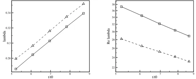
lost (at least for what concern the order of magnitude and behavior required for scales considerations, see figure 2.3.5). The Taylor microscale then grows both in time and with the position, following the decrease in energy content of the flow (figures 2.3.8and2.3.9), hence the Reλevolves accordingly. In the studied temporal range, the turbulent side λ vary from 0.26 to 0.33, while Reλ decays from 37 to 28.

t/t0 la m b d a 5 6 7 8 9 0.28 0.3 0.32 0.34 t/t0 R e la m b d a 5 6 7 8 9 22 24 26 28 30 32 34 36 38

Figure 2.3.8: Evolution of the Taylor microscale λ (left) and Reλ (right). Solid line: tur-bulent core, dashed: interface (x = 0)

Evidently the Kolmogorv scale η = (v3_/ϵ)1/4_{, grows spatially moving toward the}

irrota-tional flow following the decrease in energy content of the flow (figure 2.3.9), though the evolution of the Kolmogorov scale has a much smoother profile. To note that η highlights a steep decay of the small scales in the interface region.

2.3.3

Enstrophy and energy scales

As introduced in the first chapter, one of the essential quantitative markers of turbulence is vorticity. The square of the vorticity divided by two is called enstrophy and is a quantity useful for characterizing a variety of turbulent phenomena. Moreover enstrophy thresholds has been often used as detection mechanism for the turbulent/non-turbulent interface (see Holzner et al. 2006, 2007), since a sharp jump in enstrophy levels can be observed crossing the interface.

x la m b d a -1.5 -1 -0.5 0 0.3 0.31 0.32 x et a -1.5 -1 -0.5 0 0.03 0.04 0.05 0.06 0.07 0.08

Figure 2.3.9: Spatial variation of the Taylor microscale λ (left) and Kolmogorov sale η (right). t/t0 =6.9 x -1 0 1 0 3 6 9 12

Figure 2.3.10: Temporal evolution of enstrophy ⟨

ω2

i

2

⟩

,solid line: t/t0 =5.2 , dashed 6.0,

Figure 2.3.10 shows the averaged profiles of enstrophy across the interface. The graph show as enstrophy decrease to a zero level in the non-turbulent side, while it has a quasi-constant value in the turbulent side of the field. The enstrophy follows the same profiles observed in previous experiments with grid induced turbulence ( Holzner et al. 2007) and DNS of wakes ( Bisset et al. 2001).

The simulation of the Navier-Stokes equation in the Fourier space give an easy way to compute both energy and enstrophy spectra of the field. In fact if the Fourier coefficient ˆ

ui(kx, ky, kz) and ˆω(kx, ky, kz) are known, the spectrum can be obtained by multiplying each term for its complex conjugate. In the present study the spectra has been evaluated in each section y-z of the field, to evaluate the distribution of energy and enstrophy in both the longitudinal direction and plane wave numbers ky − kz, thus obtaining the functions

Ek(x, ky, kz) and Ωk(x, ky, kz). Since the flow is isotropic in the y-z planes, we will con-sider the integral of the spectral energy and enstrophy over a circular shell in the ky− kz space, i.e Ek(x, k) and Ωk(x, k).

The plot of Ek (figure 2.3.11) highlights three different behaviors. The first one is that across the interface persists an intermediate range of scales which retains energy levels comparable with the ones found into the turbulent core. The second and the third one is a larger and smaller decrease of energy at small and large scale respectively, crossing the interface. This behavior may be induced by the combination of two effects. The first one could be the erosion of small scales due to dissipation which persists crossing the interface as will be shown in the spectral enstrophy after. The second could be the orientation of the spatial energy fluxes from the turbulent core towards large scale motion. It is interesting to note that the protrusion of large scale fluctuations, which have a much lower spatial decay with respect all the other scales, is characterized essentially by irrotational motion as will shown below whit spectral enstrophy.

The spectral enstrophy Ωk (figure 2.3.12) have a much flatter spatial decay confronted to the kinetic energy spectra, i.e. all the scales exhibit nearly the same decay along x. The comparison between the kinetic energy spectrum and the enstrophy spectrum indicate a higher dissipation of kinetic energy at small scales, which correspond to a slow spatial decay of enstrophy levels in such region. The decay of large scale of enstrophy with x indicates that the large scale protrusions seen in the energy spectra are probably due to irrotational velocity fluctuations in the laminar flow.

x lo g (k ) -1.5 -1 -0.5 0 0.5 1 1.5 0 1 2 3 4 logE -5.8 -7.35 -8.9 -10.45 -12 x lo g (k ) -1.5 -1 -0.5 0 0.5 1 1.5 0 1 2 3 4 logE -5.8 -7.35 -8.9 -10.45 -12

x lo g (k ) -1.5 -1 -0.5 0 0.5 1 1.5 0 1 2 3 4 Enstrophy -1 -2 -3 -4 -5 -6 -7 -8 -9 -10 x lo g (k ) -1.5 -1 -0.5 0 0.5 1 1.5 0 1 2 3 4 Enstrophy -1 -2 -3 -4 -5 -6 -7 -8 -9 -10

2.3.4

Enstrophy balance equation

Entrainment is a process where turbulence generates other turbulence in an irrotational re-gion, hence the study of the local production or dissipation of vorticity helps to understand the mechanics of the underlying entrainment process. The equation for the local balance of enstrophy is 1 2 D Dt ⟨ ω_i2⟩=⟨ωiωjsij⟩ + ν ⟨ ωi∇2ωi ⟩ (2.3.4) where the term sij is the strain rate and is given by

sij = 1 2 ( ∂ui ∂xj +∂uj ∂xi ) . (2.3.5)

The first right-hand side term of the 2.3.4 is the turbulent stretching of fluctuating vortic-ity while the second term on the right is the viscous dissipation; re-expressing the total derivative, equation 2.3.4 becomes

1 2 ∂ ∂t ⟨ ω_i2⟩+1 2 ⟨ uj ∂ ∂xj (ω2_i) ⟩ =⟨ωiωjsij⟩ + ν ⟨ ωi∇2ωi ⟩ . (2.3.6)

The second term on the left side can be also written as ⟨ uj ∂ ∂xj (ω2_i) ⟩ =− ∂ ∂xj ⟨ ω_i2uj ⟩ + ⟨ ω2_i∂uj ∂xj ⟩ , (2.3.7)

we have hence that the left side of the equation can be written as

1 2 ∂ ∂t ⟨ ω2_i⟩+1 2 ⟨ uj ∂ ∂xj (ω_i2) ⟩ = 1 2 ∂ ∂t ⟨ ω2_i⟩+1 2 ⟨ ∂ ∂xj (ω_i2uj) ⟩ − 1 2 ⟨ ω2_i∂uj ∂xj ⟩ . (2.3.8)

The last term is zero due to the zero-divergence of the velocity field, thus we have that the enstrophy evolution is 1 2 ∂ ∂t ⟨ ω_i2⟩ =−1 2 ⟨ ∂ ∂xj (ω_i2uj) ⟩ +⟨ωiωjsij⟩ + ν ⟨ ωi∇2ωi ⟩ . (2.3.9)

⟨ ωi ∂2_ω i ∂x2 j ⟩ =− ∂ 2 ∂x2 j ⟨ ω2_j⟩+ 2 ⟨ ∂ωi ∂xj ∂ωi ∂xj ⟩ , (2.3.10)

the consequence is that

ν⟨ωi∇2ωi ⟩ = ν 2 ∂2 ∂x2 j ⟨ ω_j2⟩− ν ⟨ ∂ωi ∂xj ∂ωi ∂xj ⟩ , (2.3.11)

thus the final relation for the enstrophy balance equation is

1 2 ∂ ∂t ⟨ ω_i2⟩=−1 2 ∂ ∂xj ⟨ ω_i2uj ⟩ +⟨ωiωjsij⟩ + ν 2 ∂2 ∂x2 j ⟨ ω2_i⟩− ν ⟨ ∂ωi ∂xj ∂ωi ∂xj ⟩ . (2.3.12)

This last relation evidence how the evolution of enstrophy is the result of four contributes. The term ν ⟨ ∂ωi ∂xj ∂ωi ∂xj ⟩

is always definite positive hence its contribute to enstrophy balance is dissipative, that is why it is usually called viscous dissipation. The term ν_2∂x∂22

j

⟨

ω2

j ⟩ represents the diffusion of vorticity due the viscosity. Must be noted that the decomposition in 2.3.11 is not unique, there is an infinite number of possibilities to represent ν⟨ωi∇2ωi⟩ as a sum of a dissipation and a flux term (i.e. as a divergence of some vector) (Holzner 2007). There is no way to define dissipation (i.e. to choose one among many purely negative expressions) of enstrophy as it is not an inviscidly conserved quantity, unlike the kinetic energy (Tsinober 2001). Nevertheless such decomposition retain its utility in understanding some of the underlying physical aspects of turbulent diffusion, as will be seen soon.

The term⟨ωiωjsij⟩ is responsible for enstrophy production and arises from the interactions between the vorticity and the rate of strain tensor sij. It is usually considered as a positive term, although so far no theoretical arguments in favor of positiveness of ⟨ωiωjsij⟩ have been given (Tsinober 2001). Last, the term −1_2∂x∂

j ⟨ω

2

iuj⟩ is the gradient of the

interac-tions between vorticity and velocity fluctuainterac-tions, represent how vorticity is transported by velocity fluctuations and we will call it inertial diffusion. Our data are averaged in the

y− z planes, where homogeneity is conserved. Thus equation 2.3.12 retains only the x

1 2 ∂ ∂t ⟨ ω_i2⟩ =−1 2 ∂ ∂x ⟨ ω2_iuj ⟩ +⟨ωiωjsij⟩ + ν 2 ∂2 ∂x2 ⟨ ω_i2⟩− ν ⟨ ∂ωi ∂xj ∂ωi ∂xj ⟩ . (2.3.13)

In the case of decaying turbulence the global balance lead to a continuous dissipation of vorticity due to the viscosity. Nevertheless in our case, where the entrainment is undergo-ing, there should be zone of positive variation of vorticity _∂t∂ ⟨ω2

i(x)⟩ > 0. This positive variation, in a globally turbulence-decaying frame,(figure 2.3.13) can be only attributed to the entrainment of irrotational fluid in the turbulent mass and permits to identify where the entrainment rate reaches its maximum, see inset of figure 2.3.13

x -1.5 -1 -0.5 0 0.5 1 1.5 -80 -60 -40 -20 0 0.4 0.6 0.8 -0.4 -0.2 0 0.2

Figure 2.3.13: Plot of the term 1_2∂t∂ ⟨ω2_i⟩, time step from t/t0=5.2 (lowest level) to 8.6. In

the magnification the zone of positive enstrophy variation.

The position of such maxima results to be forward respect the points at 10% threshold of enstrophy shown in figure2.3.23 and forward respect the peaks of inertial and viscous diffusion that will be shown in what follows.

Figure 2.3.15 illustrate the components of enstrophy production for t=2.0. As mentioned above the production term is positive in all the field, due to the fact that turbulence is

de-t/t0 x 5 5.5 6 6.5 7 7.5 8 8.5 0.5 0.55 0.6

Figure 2.3.14: Position of the enstrophy balance maximum.

caying, it is about a half of the dissipation term. The latter dominate the enstrophy balance equation in the turbulent core, only in the outbounds of the interface region it reaches val-ues comparable with the three other terms. More intersting are the terms of viscous and inertial transport since these terms are responsible for the advancement of the interface. These two terms start rising while getting closer to the interface and slowly return to zero once crossed it. The inertial term result always sensibly greater then the viscous term and , around the interface, it result greater then the production term. This suggest that in such region, the transport by velocity of vorticity prevails over the amplifying interactions between vorticity field and strains.

The net fluxes of both the inertial and viscous diffusion have been analyzed in order to better understand the contribution in turbulent entrainment. The results are illustrated in figure 2.3.16 where the dominance of the inertial flux over viscous flux is evident. The inertial flux thus draws vorticity from the turbulent core and transports it toward the inter-face, before which it reaches its maximum. The viscous flux remains at least one order of magnitude less than the inertial flux and reach its maximum intensity slightly closer to the laminar field. Hence from this picture it appears that inertial fluctuations plays a central

x -1.5 -1 -0.5 0 0.5 1 1.5 -30 -20 -10 0 10 x -1.5 -1 -0.5 0 0.5 1 1.5 -1 0 1

Figure 2.3.15: Enstrophy balance terms. Solid line: production ⟨ωiωjsij⟩, dashed line: dissipation term−ν ⟨ ∂ωi ∂xj ∂ωi ∂xj ⟩

, dotted line: inertial diffusion−1_2∂x∂ ⟨ω2_iu⟩, dashed and

dot-ted line: viscous diffusion ν_2∂x∂22 ⟨ω 2

i⟩. (below) Magnification of the inertial and viscous

role in transporting rotational flow from the high turbulence levels of the core toward the interface. Whereas, at the interface the intensity of the fluctuations is small and the prop-agation of rotational fluid toward the laminar region become a mechanism dominated by molecular viscosity. x -1.5 -1 -0.5 0 0.5 1 1.5 0 1 2 3 4

Figure 2.3.16: Viscous flux ν_2∂x∂ ⟨ω2

i⟩ (solid line) and inertial flux −

1 2⟨ω

2

iu⟩ (dash-dotted

line). t/t0=8.6

The temporal variation of inertial flux (figure 2.3.17, left) does not evidence a signifi-cant movement of its peaks, confirming that the dependence of this process on the inertial mechanisms of the the turbulent core, which position remain unaltered in time. The analy-sis of the components of the inertial flux (figure 2.3.17, right) shows as expected stronger contribution of the terms of transversal vorticity. These are responsible in generating the convoluted protrusion of vorticity which can be seen in the interface visualizations. Previ-ous authors reported the inertial flux to be globally zero at the interface for entrainment in jets (Westerweel et al. 2009). The inertial component v· ω2_z has been obtained by the PIV measure of the planar vorticity and velocity fields. The pdf of such component evidenced a strongly intermittent but symmetrical profile. The authors hypothesized than that at the interface, the contribution two of counterotating adjacent vortexes would lead to a zero inertial flux (as seen in figure 2.3.18).

In our simulation a relevant flux of inertial transport has been found and also the pdf of the inertial term seems to confirm it. The longitudinal term−1₂⟨ω2

x -1.5 -1 -0.5 0 0.5 1 1.5 0 1 2 3 4 x -1.5 -1 -0.5 0 0.5 1 1.5 0 0.1 0.2 0.3

Figure 2.3.17: (Right) Temporal evolution of the inertial flux, from t/t0= 1.2 (highest level)

to 8.6. (Left) Components of the inertial flux: Solid line:−1₂ ⟨ω_x2u⟩ , dotted line:−1₂⟨ω2_yu⟩

, dash-dotted line−1₂⟨ω2

zu⟩ . t/t0= 8.6 .

Figure 2.3.18: Example of the contribution of the vorticity component ωz at the interface (Westerweel 2009)