INDEX
INDEX ... 1
RESUME ... 3
1 FOREWORD ... 13
2 TASK: TERRESTRIAL PLANETS’ ATMOSPHERES ... 17
2.1 VENUS... 18
2.1.1 The Atmosphere of Venus ... 23
2.1.2 The Sulphuric Acid Clouds of Venus ... 26
2.1.3 Winds on Venus ... 29
2.2 MARS... 32
2.2.1 The Martian atmosphere: gaseous components ... 33
2.2.2 Dust... 39
2.2.3 Main phenomena of Martian atmosphere ... 41
3 TOOLS: SPECTROMETERS AND INFRARED SPECTROSCOPY... 47
3.1 THE INSTRUMENT: VIRTIS - VEX ... 49
3.1.1 Venus Express mission ... 49
3.1.2 The Visible and Infrared Thermal Imaging Spectrometer ... 49
3.1.3 VIRTIS technical specifications... 55
3.2 THE INSTRUMENT: PFS - MEX ... 57
3.2.1 The Planetary Fourier Spectrometer experiment (PFS) ... 57
3.2.2 General instrumental set-up... 57
3.2.3 Examples of PFS Martian spectra ... 62
3.3 IR SPECTRA OF A PLANETARY ATMOSPHERE... 66
3.3.1 Basic definitions... 66
3.3.2 Effects of surface... 68
3.3.3 Microscopic effects of gases... 71
3.3.4 Microscopic effects of aerosols ... 75
3.3.5 Macroscopic description... 76
3.3.6 Total field ... 81
4 GENERAL RETRIEVAL METHOD ... 85
4.1 INTRODUCTION... 85
4.2.1 Radiative transfer without scattering ... 93
4.2.2 Radiative transfer with multiple scattering ... 96
5 RESULTS FOR VENUS ... 99
5.1 VENUS SPECTRA COMPUTATION TO MODEL VIRTIS-M DATA... 100
5.1.1 Models for night side spectra in the region 3.5 – 5.0 µm ... 101
5.1.2 Test: comparison of CO2 spectroscopic databases ... 102
5.1.3 Choice of the monochromatic grid ... 104
5.1.4 Test of different CO2 line cutoff ... 106
5.1.5 Test of different radiative transfer options for the treatment of scattering 107 5.1.6 Validation of a fast direct RT method for the retrieval of the atmospheric temperature profile ... 108
5.2 TASK: SEARCH FOR WATER IN VENUS ATMOSPHERE... 111
5.2.1 Water from VIRTIS M data ... 112
5.2.2 Water from VIRTIS H data ... 115
5.2.3 Atmospheric model... 123
5.2.4 Retrieval method... 126
5.2.5 Results for the cloud tops altitude... 134
5.2.6 Results for water abundance... 140
5.2.7 Inverse Method... 146
6 RESULTS FOR MARS... 153
6.1 CARBON MONOXIDE ABUNDANCE (CO) IN MARTIAN ATMOSPHERE... 154
6.1.1 Retrieval method and Atmospheric model ... 156
6.1.2 Data... 160
6.1.3 Error evaluation... 160
6.1.4 Results... 163
6.1.5 Discussion ... 169
6.2 CO2 ISOTOPES RETRIEVAL IN MARTIAN ATMOSPHERE... 171
6.2.1 Data... 172
6.2.2 Retrieval method and Atmospheric model ... 173
6.2.3 Results on isotopic abundances... 175
6.2.4 Discussion ... 190
7 CONCLUSIONS ... 193
Resume
This work presents part of the efforts which I carried out in the Interplanetary Space Physics Institute (IFSI) and in the Cosmic Physics and Space Astrophysics Institute (IASF) of the Italian National Institute for Astrophysics (INAF) in the analysis of the data from the Planetary Fourier Spectrometer (PFS) experiment, included in the scientific payload of the ESA Mars Express (MEX) mission to Mars and the Visual and Infrared Thermal Imaging Spectrometer (VIRTIS) experiment, included in the ESA Venus Express (VEX) mission to Venus.
Information obtained from the study of terrestrial planets are fundamental for the understanding of Earth past and future climate evolution, since other terrestrial planets represent in some sense a possible stage – or alternative path - of the Earth’s history.
The study of our closest neighbors, Mars and Venus, gives important information also in the search for planets belonging to other planetary systems - which is one of the mayor current interest of the scientific community - in order to provide a paradigm about planets orbiting around other stars, and which may possibly host life.
Mars and Venus pertain to the planets with a “CO2 dominated”
atmosphere and since they experiment different atmospheric conditions they provide an unique chance to obtain complete information on this atmospheric type at different evolutional stages (in Chapter 2 a brief description of the two planet atmospheres is presented).
In particular, using the data acquired by the two ESA spacecraft we investigated the atmospheric composition of the two planets in order to give a contribute to the understanding of the main properties of Mars and Venus, since the composition of the atmosphere on global and regional scales influences the planetary climate and the evolution and the retrieved
information can therefore be used to trace the atmospheric circulation, give constraints to the atmospheric stability and its long term evolution.
Efforts have focused on topics still affected by large uncertainties in our understanding of atmospheric constituents other than carbon dioxide, in order to provide also firm constraints for future studies on atmospheric aeronomy and interaction with surface phenomena such as volcanism and related outgassing.
Namely, for this task we had the first chance to perform an intensive study of water vapor on Venus (previous studies regarded just limited local time or locations in the planet), since the role of water as a trace constituent is key to illuminating the present-day Venus atmospheric energy balance, particularly with respect to the global cloud layers which permanently envelop the planet.
On Mars we investigated the stable isotope record contained within carbon and oxygen (CO2 isotopes), to provide important constraints regarding the origin of the planet and its relationship to the Earth. Stable oxygen isotopes are particularly useful in the study of Mars because oxygen is abundantly present in both the Martian atmosphere and lithosphere, in particular in the main atmospheric constitute, carbon dioxide. We also investigated carbon monoxide (CO) on Mars, since it represents the main product of the CO2 photolysis and therefore is directly related to the
problem of the stability of the Martian CO2 atmosphere.
Infrared spectroscopy and present-day high resolution spectrometers have demonstrated to be one of the most powerful remote sensing tools in the context of planetary observation, for atmospheric as well as for surface studies: they give together a remote access to most of the important information carried by the radiation which directly interacted with the planet.
cover the main roto-vibrational bands of several molecules being present in planetary atmospheres, so that at the present time, most of our knowledge regarding planetary atmospheric composition and structure has been achieved by remote sensing spectroscopy.
Since the IR radiation emerging from a planetary atmosphere it is described from the Radiative Transfer equation, we presented (Chapter 3) some basic principles of the theory of radiative Transfer in the appropriate form for planetary atmospheres.
Once we have available the infrared spectra of Mars and Venus acquired by PFS and VIRTIS, we need to produce models which properly describe (simulate) what the instrument measures, in order to retrieve from the spectra the required quantities, namely composition.
Many factors contribute to the formation of a spectrum emerging from a planet: the chemical and physical state of the surface, the atmospheric composition and thermal structure, the aerosols content and their nature, the observational and illumination geometry (emission, incidence and phase angles) and also the instrumental properties as the response function and resolution, since our measured spectrum consist actually in the convolution of the radiance with the instrumental function.
We need to take into account all these factors when working to model the atmospheres and the radiance spectra emerging from it.
We have illustrated (in chapter 4) methods and models we used and built with the aim of computing synthetic spectra, which are essential for comparison with the data produced from the instruments and which occupied an essential and demanding part of this study.
We have described the analytic techniques for the resolution of the radiative transfer equation, discussing not only the basic background but also the practical choices made to solve the various physical equations; the main mathematical equations required for the retrieval of atmospheric state observed by the instruments were also introduced.
Afterwards we presented the specific methods and results for Venus (chapter 5), including a description of the first approach we had on
modelling the Venus atmosphere due to the importance the methodology development had in this work for the achievements of our tasks; we described then the specific task in the investigation of this planet, i.e.: the water content and its variation in the mesosphere, just above the thick Venusian clouds of sulphuric acid. After showing the atmospheric model developed to solve the RT equation, we explained the retrieval methods which we implemented to analyse the atmospheric quantities.
This last topic has been very interesting and instructive since I had to completely create the code which was used for the automatic and extensive retrieval and analysis of the Venusian cloud top altitude (to determine the correct atmospheric pressure and optical path) simultaneously to the retrieval of the water vapour above the clouds, with all this performed on individual spectra and for all the available data. Results obtained with this method were then interpreted, validated and a formal inverse method to quantify the errors was implemented too.
We have described (chapter 6) both the methods and results obtained for Mars, with the task of investigating the CO2 isotopomers ratio in the
atmosphere and the content of carbon monoxide, important tracers of atmospheric physical and dynamical phenomena.
This last part describes more briefly the model developed to simulate the Martian spectrum and the methods to retrieve the physical quantities - since the retrieval procedure are similar (despite the model changes completely) to the ones used to study Venus atmosphere - to quickly arrive to the presentation of the results.
Results
The water vapor abundance in the mesosphere of Venus has been already measured in a number of ground-based and spaceborn experiments. Various experiments gave approximately the same values from several ppm to a bit more than 10 ppm. An intriguing exception was the strong local enhancement up to 102 ppm soon after the subsolar point
in the equatorial region observed by the Pioneer Venus OIR (Schoefield et al., 1982; Irwin et al., 1997; Koukouli et al., 2005). Thus our present study had two main goals: to measure the water vapor abundance at the cloud tops with high spatial resolution, and to search for the wet spots observed by the Pioneer Venus. As a byproduct we measured the cloud top altitude.
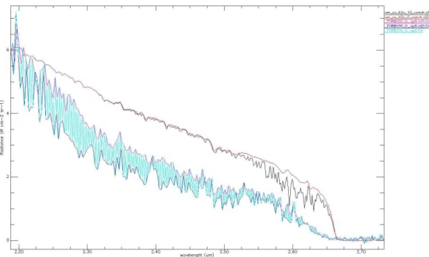
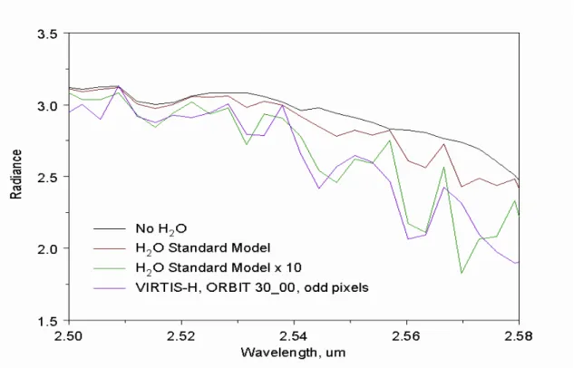
The Venus Express and VIRTIS observation strategy was particularly favorable for measurements at low latitudes around noon. Here the water vapor abundance near cloud top level at 2.5 µm was found to be 6 ± 2 ppm. Our best horizontal spatial resolution was about 10 km on the cloud “surface”, giving for the first time the chance with our high spatial resolution to measure local variations.
Pixel-to pixel variations were within 20% and do not exceed random measurement error. Thus we did not observe any anomalously wet regions reported by the Pioneer Venus OIR experiment team. To be precise we have to note that the cloud top region in the far IR is located lower by several kilometers than that at 2.5 µm, and therefore we were sensitive to a higher level of atmosphere. The level of maximum sensitivity to the variations of water vapor is equal to 68 km, the corresponding cloud top altitude at 1.5 µm being equal to 75 ±1 km.
We observed an increase of water vapor abundance up to 20 ppm near both morning and evening terminator. However, the result is highly sensitive to the absolute precision of the continuum level calibration, since
in this region the intensity of outgoing radiation is low due to high incidence solar angle. With the instrumental uncertainties related to the removal of the dark current and absolute calibration of the VIRTIS-H spectra, a systematic bias is possible. Thus this result needs additional confirmation.
The future attempts should be devoted to the improvements of spectral and radiometric calibration of the VIRTIS-H & M instruments to get rid of the possible systematic biases related to calibration uncertainties and to increase the data amount suitable for studies of minor species. A next step would be a complex high spatial resolution study of water vapor abundance and its correlation with cloud properties, UV absorber, and abundances of other minor species.
Results show a CO mixing ratio with an average value of about 800 ppm from a first analyzed dataset observations acquired in a latitude range of approximately (- 60) ÷ (+ 60) degrees and in a solar longitude range which encompass the summer and the beginning of autumn in the northern hemisphere, therefore winter in the southern one (Ls range: 90° - 200°). Higher average values of about 900 ppm are found in the second dataset which comprises observations at the end of winter and beginning of spring in the north hemisphere (Ls range: 330° - 95°).
Since the two datasets differ in the atmospheric model (used temperature-pressure profile), absolute values of CO atmospheric content may depend on the model. For this reason besides reporting both results of absolute CO content values, which anyway are comparable within the computed errors, we particularly stress the observed variability and trends.
From the analysis of carbon monoxide in Martian atmosphere it appears a variability of the CO content at different atmospheric conditions (25 % for a first dataset, 35% for a second), however not so strong in percentage as resulted from other studies (e.g. Billebaud et al. – 1998, which attributed to the range of CO variability values from 0 to 100%).
In fact the eddy diffusion coefficient is K ≈ 106 cm2 s-1 in Mars’ troposphere
[Korablev et al., 1993], and the vertical mixing time H2/K is two weeks (H
is the scale height). Being this mixing time much shorter than CO lifetime, carbon monoxide should be vertically well mixed.
Our results confirm this observation; we however stress that we did not yet study observations in proximity of great volcanoes, where mixing ratio could possibly vary in case of founding outgassing processes. Due to the PFS high spatial resolution, as soon as calibration over high elevated Martian features will be improved, the study of carbon monoxide over a higher altitude range will give further clarifications on previous results indicating altitude’s dependence (Rosenqvist et al., 1992)
We observe an absence of strong diurnal CO variability in agreements with models predicting the CO lifetime to be equal to 6 years, assessing for diurnal variations a very low range.
The however observed low variations with local time suggest a weak enhance on midday, where the Sun is high and the photolysis rate is more efficient.
There is an evident correlation with the Sun incidence angle. From both analyzed dataset we can observe a decrease of CO mixing ratio increasing the incidence angle.
This trend may be correlated with the energy present in the atmosphere depending on solar illumination, which could enhance CO production when the incident solar beams density is higher (small angles).
The main observed correlation is however with latitudes closer to the subsolar point in a given season. Mars Express satellite elliptical and not Sun synchronous orbits, bring to a not unimportant bias for observations in Ls (season), Latitude and Local Time, which can affect the dataset and consequently the interpretation of the variability.
Due to the mentioned bias we can mainly attribute the CO variations with incidence angle to the latitudinal dependence on the subsolar point. The observed trend of mixing ratio versus Latitude presents a maximum around latitudes in which the Sun rays meet the surface with the minimum angle in the considered season. We can observe a maximum at
low latitudes in the southern hemisphere winter, which could be correlated with CO2 decreasing due to intense condensation of CO2 on the
south polar cap.
In this case, the actual CO column density does not vary, but what changes is the mixing ratio which is related to the total atmosphere (almost totally made of CO2 in Martian case). In fact condensation and
sublimation of CO2 result in enhancement and depletion, respectively, in
the mixing ratios of incondensable species like CO.
Summarizing results on carbon monoxide, we find an increase in the
Southern winter and at the latitudes of subsolar point where solar flux is higher and therefore CO2 photolysis is more efficient. In general seasonal features are more pronounced at equatorial latitudes and meridian profiles of the mixing ratio (for individual orbits) present seasonal shift of the maximum versus the sub solar point. We find an enhancement also at low incidence angles and at midday local time.
Results on CO2 isotopes consisted primarily in the identification of all the
CO2 isotopes in PFS data (LWC), with an instrumental spectral resolution
never available before.
The retrieved abundances of the main isotopes outside the center of the main CO2 absorption band at 667 cm–1 (LWC) resulted to be close to
terrestrial values and are reported and are presented in Table 1 in the form of isotopic ratios.
Isotopic ratio
12C/13C = 82.4 16O/18O = 479.5 16O/17O = 2437.9
with the 627- which gives indication of the CO2 oxygen isotope’s content)
at different wavelengths: at 576 cm-1 is similar to the terrestrial value,
while in the bottom of the band (663 cm-1) it is found to be a little higher.
From the last spectral range even the 627 isotope seems to have much higher abundance than terrestrial value.
The retrieved abundance of 628 in the SWC (the band at 2614 cm-1) is
about 0.8 times the terrestrial value. In general, the quantity retrieved from this spectral range pertains to the atmospheric mass of the first scale height of the atmosphere.
For this reason, a realistic interpretation of the results of this study can be a variability of mixing ratio of the oxygen isotopes with the altitude. We pass from a lower value obtained in the first layers of the atmosphere (from SWC), less then terrestrial value, to values similar to the terrestrial one from the ranges of the band in LWC pertaining an altitude around 20-30 Km, to higher values in the center of the band which probes an altitude around 30-50 Km. This decreasing trend with altitude could be explained by the escape of lighter isotopes from the top of the atmosphere, with enrichment of the heavier ones going closer to the surface. Anyway some further considerations should be developed.
The column CO2 abundance in the Martian atmosphere is 2×1023 cm−2,
the column photolysis rate is 1012 cm−2 s−1. Their ratio is the mean CO2
lifetime relative to chemical processes which is 6000 years. Local lifetimes may be shorter or longer; for example, the CO2 lifetime is 30 years at 80
km. Mixing time is H2/K where H is the scale height and K is eddy
diffusion. Mixing time varies from two weeks in the lower atmosphere to 15 hours at 80 km. Mixing time is very much shorter than the chemical lifetime of CO2; therefore all CO2 isotopes should be well mixed in the
atmosphere and the CO2 isotope ratios do not depend on height up to a
homopause at 120-135 km where the diffusive separation begins.
The 628 abundances obtained in this study from various bands are 1.01 ± 0.40, 1.20 ± 0.50, 1.10 ± 0.46, and 0.8 ± 0.20. The uncertainty intervals for all values are well overlapping, and we can calculate a weighted-mean value which is equal to 0.91 ± 0.18.
The weighted-mean abundances of the other isotopes are 1.10 ± 0.35 for 636 and 1.21 ± 0.63 for 627. The abundance of 627 is equal to square root of 628 for mass-dependent fractionation, that is, 0.95 ± 0.42. The abundance of 638 is equal to product of 636 and 628, that is, 1.00 ± 0.38. The former agrees with the measured value within their uncertainties, the latter perfectly fits the measured value.
For the above reasons, without further information, we can conclude that retrieval of CO2 isotopic abundance performed from the short and long
wavelength channel of PFS spectrometer suggest results close to “terrestrial one” with a weighted-mean value which is equal to 0.91 ± 0.18.
1
Foreword
This work presents part of the efforts which I carried out in the Interplanetary Space Physics Institute (IFSI) and in the Cosmic Physics and Space Astrophysics Institute (IASF) of the Italian National Institute for Astrophysics (INAF) in the analysis of the data from the Planetary Fourier Spectrometer (PFS) experiment, included in the scientific payload of the ESA Mars Express (MEX) mission to Mars and the Visual and Infrared Thermal Imaging Spectrometer (VIRTIS) experiment, included in the ESA Venus Express (VEX) mission to Venus.
Information obtained from the study of terrestrial planets are fundamental for the understanding of Earth past and future climate evolution, since other terrestrial planets represent in some sense a possible stage – or alternative path - of the Earth’s history.
The study of our closest neighbors, Mars and Venus, also gives important information for the search for planets in other planetary systems - which is one of the mayor current interest of the scientific community - in order to provide a paradigm about planets orbiting around other stars, and which may possibly host life.
Mars and Venus pertain to the planets with a “CO2 dominated”
atmosphere and since they experiment different atmospheric conditions they provide an unique chance to obtain complete information on this atmospheric type at different evolutional stages (in Chapter 2 a brief description of the two planet atmospheres is presented).
In particular, using the data acquired by the two ESA spacecraft we investigated the atmospheric composition of the two planets in order to give a contribute to the understanding of the main properties of Mars and Venus, since the composition of the atmosphere on global and regional scales influences the planetary climate and the evolution and the retrieved
information can therefore be used to trace the atmospheric circulation, give constraints to the atmospheric stability and its long term evolution.
Efforts have focused on topics still affected by large uncertainties in our understanding of atmospheric constituents other than carbon dioxide, in order to provide also firm constraints for future studies on atmospheric aeronomy and interaction with surface phenomena such as volcanism and related outgassing.
Namely, for this task we had the first chance to perform an intensive study of water vapor on Venus (previous studies regarded just limited local time or locations in the planet), since the role of water as a trace constituent is key to illuminating the present-day Venus atmospheric energy balance, particularly with respect to the global cloud layers which permanently envelop the planet.
On Mars we investigated the stable isotope record contained within carbon and oxygen (CO2 isotopes), to provide important constraints regarding the origin of the planet and its relationship to the Earth. Stable oxygen isotopes are particularly useful in the study of Mars because oxygen is abundantly present in both the Martian atmosphere and lithosphere, in particular in the main atmospheric constitute, carbon dioxide. We also investigated carbon monoxide (CO) on Mars, since it represents the main product of the CO2 photolysis and therefore is directly related to the
problem of the stability of the Martian CO2 atmosphere.
Infrared spectroscopy and present-day high resolution spectrometers have demonstrated to be one of the most powerful remote sensing tools in the context of planetary observation, for atmospheric as well as for surface studies: they give together a remote access to most of the important information carried by the radiation which directly interacted with the planet.
cover the main roto-vibrational bands of several molecules being present in planetary atmospheres, so that at the present time, most of our knowledge regarding planetary atmospheric composition and structure has been achieved by remote sensing spectroscopy.
Since the IR radiation emerging from a planetary atmosphere it is described from the Radiative Transfer equation, we presented (Chapter 3) some basic principles of the theory of radiative Transfer in the appropriate form for planetary atmospheres.
Once we have available the infrared spectra of Mars and Venus acquired by PFS and VIRTIS, we need to produce models which properly describe (simulate) what the instrument measures, in order to retrieve from the spectra the required quantities, namely composition.
Many factors contribute to the formation of a spectrum emerging from a planet: the chemical and physical state of the surface, the atmospheric composition and thermal structure, the aerosols content and their nature, the observational and illumination’s geometry (emission, incidence and phase angles) and also the instrument’s properties as the response function and resolution, since our measured spectrum consist actually in the convolution of the radiance with the instrumental function.
We need to take into account all these factors when working to model the atmospheres and the radiance spectra emerging from it.
We have illustrated (in chapter 4) methods and models we used and built with the aim of computing synthetic spectra, which are essential for comparison with the data produced from the instruments and which occupied an essential and demanding part of this study.
We have described the analytic techniques for the resolution of the radiative transfer equation, discussing not only the basic background but also the practical choices made to solve the various physical equations; the main mathematical equations required for the retrieval of atmospheric state observed by the instruments were also introduced.
Afterwards we presented the specific methods and results for Venus (chapter 5), including a description of the first approach we had on
modelling the Venus atmosphere due to the importance the methodology development had in this work for the achievements of our tasks; we described then the specific task in the investigation of this planet, i.e.: the water content and its variation in the mesosphere, just above the thick Venusian clouds of sulphuric acid. After showing the atmospheric model developed to solve the RT equation, we explained the retrieval methods which we implemented to analyse the atmospheric quantities.
This last topic has been very interesting and instructive since I had to completely create the code which was used for the automatic and extensive retrieval and analysis of the Venusian cloud top altitude (to determine the correct atmospheric pressure and optical path) simultaneously to the retrieval of the water vapour above the clouds, with all this performed on individual spectra and for all the available data. Results obtained with this method were then interpreted, validated and a formal inverse method to quantify the errors was implemented too.
We described (chapter 6) both the methods and results obtained for Mars, with the task of investigating the CO2 isotopomers ratio in the atmosphere
and the content of carbon monoxide, important tracers of atmospheric physical and dynamical phenomena.
This last part describes more briefly the model developed to simulate the Martian spectrum and the methods to retrieve the physical quantities - since the retrieval procedure are similar (despite the model changes completely) to the ones used to study Venus atmosphere - to quickly arrive to the presentation of the results.
2
Task: terrestrial planets’ atmospheres
The bodies of the Solar System gradually formed and reached their current state as we observe today. These bodies started their evolution in different initial conditions in terms of composition and mass, solar distance and other parameters. Therefore it is important to follow and compare the evolutionary path of these individual objects.
Information obtained from the study of terrestrial planets are fundamental for the understanding of Earth past and future climate evolution, since other terrestrial planets represent in some sense a possible stage – or alternative path - of the Earth’s history.
The study of our closest neighbors, Mars and Venus, also gives important information for the search for planets in other planetary systems - which is one of the mayor current interest of the scientific community - in order to provide a paradigm about planets orbiting around other stars, and which may possibly host life.
For example, observations of the cloud-covered “sister planet” Venus become more and more important since Venus’s evolution and geology are very similar to Earth’s; and a deeper understanding of Venus’s geophysical and atmospheric characteristics could help us in the quest for earth-like planets. Also Venus’s notorious “runaway greenhouse effect” may offer lessons for limiting our potentially interference with our own planet’s climate, to ensure a long term perspective for life on Earth. Eventually, the study of planets as Venus and Mars can aid our understanding of terrestrial and extra-solar planet evolution, surface and interior processes, atmospheric circulation, chemistry, and aeronomy. In the following paragraphs a short introduction to Venus and Mars is given, discussing the major basic facts about the two planets, their general characteristics and their atmosphere. Extensive information can be found in Venus, 1983, Venus II, 1997 and Mars, 1993.
2.1
Venus
Venus is Earth's closest neighbor, the second planet from the Sun. Considered Earth's twin for many decades, Venus must have followed a very different evolutionary path since it exhibits almost no Earth-like characteristic other than a similar mass and radius. Its small rotation axis obliquity and orbital eccentricity ensures that no seasons affect its rocky surface where the temperatures rise to 500°C with a pressure 90 times the Earth's one. Venus atmosphere is composed almost solely of carbon dioxide and is enshrouded by sulphuric acid clouds that contribute greatly to the runaway greenhouse effect responsible for the high temperatures on its surface. These clouds also do not allow a direct view of the surface in the visible domain and actually - until the first UV telescope started looking at the planet - the complicated patterns created by the cloud motions were thought to belong to the planetary surface. Venus belongs to the family of terrestrial planets, alongside Earth, Mars and Mercury. Known since ancient times due to its brilliant color, brightness and unusual appearances in the sky, Venus is a planet similar to the Earth in mass and radius but has no moon and no magnetic field shielding it from cosmic rays and solar winds. Venus' obliquity is only 2.6°, compared to ~24° of the Earth and Mars and orbits in the prograde direction about the Sun in a nearly circular orbit every 224.7 earth days. Its rotation relative to the stars, the sidereal motion, is retrograde every 243.01 earth days. If the Sun could be seen from the surface of the planet, it would make roughly one complete circuit of the Venusian sky in half a Venus year. Hence, the length of the Venus day, also known as the solar day, is 116.75 Earth days.
Since Venus is closer to the Sun than the Earth, the planet shows phases when viewed with a telescope: sometimes it appears as a crescent, others
irrevocable piece of important evidence in favor of Copernicus's heliocentric theory of the solar system. As an inferior planet Venus revolves around the Sun faster than the Earth; and as the two planets are moving in the same direction around the Sun, Venus appears for a few months in the early morning, some hours before sunrise, then disappears only to be seen as a bright moon-like object emerging after sunset for a further few months before disappearing again.
The main orbital and solid body characteristics of Venus and Earth are given in Table 2 for easy comparison, while in Table 3 the Venusian observational parameters are presented.
Venus was explored by a fleet of American and Soviet spacecraft starting with Mariner 2 in 1962, the first successful spacecraft to fly-by Venus, up to the Magellan orbiter in 1990, which produced global detailed maps of Venus' surface using radar mapping, altimetry and radiometry techniques with a resolution of ~100 m. In between, more than twenty missions have explored Venus, including the Soviet Venera 7 in 1970 which was the first spacecraft to land on another planet, Venera 9 in 1975 which returned the first photographs of the surface and the American Pioneer Venus Orbiter in 1978 which carried several atmospheric environment experiments and four entry probes. Magellan’s observations further revealed that the surface of Venus is mostly covered by volcanic materials. Volcanic surface features, such as vast lava plains, fields of small lava domes and large volcanoes are common. A color-coded composite of these observations is shown in Figure 1. The planetary elevation is calculated over the mean radius of the planet; 6050 km. Venus has two major continents, Aphrodite Terra and Ishtar Terra, which occupy only a few percent of the total surface area. Aphrodite Terra, seen in Figure 1, is a long, narrow area which stretches over 150° in longitude and contains a few peaks higher than 8 km. Ishtar Terra contains the highest elevation region, Maxwell Montes, around 65°K which rises to altitudes of 10.5 km above mean planetary radius. The remainder of the surface of Venus is covered mostly by volcanic materials.
Venus Earth (Venus/Earth) Bulk parameters Mass (1024 kg) 4.8685 5.9736 0.815 Volume (1010km3) 92.843 108.321 0.857 Equatorial radius (km) 6051.8 6378.1 0.949 Polar radius (km) 6051.8 6356.8 0.952 Volumetric mean radius (km) 6051.8 6371.0 0.950 Ellipticity (polar flattening) 0.000 0.00335 0.0 Mean density (kg/m3) 5243 5515 0.951 Surface gravity at equator (m/s2) 8.87 9.80 0.905 Escape velocity (km/s) 10.36 11.19 0.926
Bond albedo 0.76 0.30 2.53
Visual geometric albedo 0.65 0.367 1.77 Solar irradiance (W/m2) 2613.9 1367.6 1.911 Equivalent blackbody temperature
(K)
231.7 254.3 0.911
Topographic range (km) 15 20 0.750
Orbital parameters
Semi major axis (106 km) 108.21 149.60 0.723 Sidereal orbit period (days) 224.701 365.256 0.615 Tropical orbit period (days) 224.695 365.242 0.615 Perihelion (106 km) 107.48 147.09 0.731 Aphelion (106 km) 108.94 152.10 0.716
Synodic period (days) 583.92 — —
Mean orbital velocity (km/s) 35.02 29.78 1.176 Max. orbital velocity(km/s) 35.26 30.29 1.164 Min. orbital velocity (km/s) 34.79 29.29 1.188 Orbit inclination (deg.) 3.39 0.00 — Orbit eccentricity 0.0067 0.0167 0.401 Sidereal rotation period (h) 5832. 5 23.9345 243.686 Length of day (h) 2802.0 24.0000 116.750 Obliquity (deg.) 177.36 23.45 (0.113)
Distance from Earth
Minimum (106 km) 38.2
Maximum (106 km) 261.0
Apparent diameter from Earth
Maximum (seconds of arc) 66.0 Minimum (seconds of arc) 9.7 Mean values at inferior conjunction with Earth
Distance from Earth (106 km) 41.44 Apparent diameter (seconds of arc) 60.2
Table 3. Observational parameters.
Although Venus has a dense atmosphere, the surface shows no evidence of substantial wind erosion, and there has been only slight evidence of limited wind transport of dust.
On Venus we cannot find evidence of plate tectonics (trenches, ridges), as the absence of water in the surface, which evaporated and went lost with the increase of greenhouse effect, did not help the subduction of the crust; this on the contrary induced an increase of heat which produced diffuse volcanism. Moreover on the Venus surface there is no clear distinction between basaltic (ocean) crust from continental granitic crations, as observed on our planet. The absence of craters on Venus is an indication of a young surface, which is dated no more than 1 Gy.
Figure 1. Color-coded topographic map of Venus from Magellan radar observations. Aphrodite Terra appears as the bright feature along the equator with an area the size of South America (NASA).
2.1.1 The Atmosphere of Venus
On June 6, 1761, at the University Observatory of Saint Petersburg, Russia, Mikhail Lomonosov (1711 -1765) observed a transit of Venus: a rare passage of the planet directly in front of the Sun. He was able to get a fairly good measurement of Venus' diameter and found that it was very similar to the Earth's. But the edge of Venus' disk, instead of appearing sharp, as he had expected, was fuzzy and indistinct, and a grey halo surrounded the planet. He had discovered the atmosphere of Venus and in his own words, he had found evidence of “an atmosphere equal to, if not greater, than that which envelops our Earthly sphere”.
The current atmospheric composition of Venus is dominated by CO2
(96.5%), with a few percent of N2 (3.5%) and a number of trace gases like
H20, CO and SO2 in the parts per million scale. This composition
resembles the atmosphere of Mars which is also made of C02 and N2 and
is instead very different from the terrestrial atmosphere where N2 and O2
play the leading part. The composition of the Venus’ atmospheres is tabulated in Table 4.
The high surface temperature of Venus (750 K) is significantly above its effective temperature, that is, the equilibrium temperature expected from its heliocentric distance. Indeed, the surface and the lower atmosphere of Venus have been heated by a runaway greenhouse effect, mostly to be ascribed to the large amounts of gaseous CO2 and H2O which were most
likely present in the primordial atmosphere and, in lesser part, to its cloud coverage.
Atmosphere
Surface pressure 92 bar Surface density 65 kg/m3
Scale height 15.9km
Total mass of atmosphere 4.8_1020 kg Average temperature 737K (464 1C) Diurnal temperature range 0
Wind speeds 0.3–1.0 m/s (surface) Mean molecular weight 43.45 g/mol
Atmospheric composition (near surface, by volume)
Major Carbon dioxide (CO2) 96.5%
Nitrogen (N2) 3.5%
Minor (ppm) Sulphur dioxide (SO2) 150
Argon (Ar) 70
Water (H2O) 20
Carbon monoxide (CO) 17
Helium (He) 12
Neon (Ne) 7
Table 4. Atmospheric properties and composition
Venus is covered by a thick cloud deck of sulfuric acid H2SO4, at an
altitude of 40–70 km, which prevents the visible observation of the surface (see paragraph 2.1.2).
The atmosphere of Venus may be divided into three natural regions, a troposphere (surface to 60 km), a mesosphere (60 to 90 km) and a thermosphere (above 90 km). On Earth we find a troposphere (surface to 12 km), a stratosphere (12 to 45 km), mesosphere (45 to 85 km) and, as on Venus, a thermosphere (above 85 km). Vertical profiles of temperatures on Venus and Earth as a function of pressure at 30° latitude, as measured by the Pioneer Venus OIR and Nimbus 7 spacecraft respectively, are presented in Figure 2 on the left. Throughout the troposphere and mesosphere the temperature decreases with height, from
temperature inversions can be seen since UV absorbing ozone that cause the Earth's stratosphere do not exist in the Venus' CO2 dominated
atmosphere. On Venus' dayside the temperature above 85-90 km rises to an exospheric value of around 300 K due to solar EUV absorption and therefore behaves like the thermosphere on Earth, where temperatures rise from ~ 180 K to ~ 1000 K. The nightside upper atmosphere on Venus differs from that on Earth because Venus' slow rotation period causes solar heating to be absent for far too long to maintain the high temperatures found on the dayside. Night side temperatures on Venus' thermosphere above 85-90 km in fact do not rise above 100 K, justifying the name of "cryosphere" ("sphere of cold" in Greek). The Venus temperature structure above the clouds and the thermosphere/cryosphere region is shown in Figure 2 on the right, as observed by three Pioneer probes and Venera 11 and 12.
Figure 2. Left. Vertical profiles of temperature vs. pressure at 30°N latitude, as measured on Venus by PV OIR and on Earth by Nimbus 7. Adapted from Houghton et al. (1984). Right. Temperatures above the main cloud regions derived from three Pioneer probes and Venera 11 and 12. Adapted from Seiff (1983).
Due to its slow rotation rate and its obliquity, the troposphere of Venus is almost isothermal in equatorial and middle latitudes. Near the poles of Venus, starting at 60° N, a long-lived dramatic instability occurs, known as the “polar collar” (or cold collar), which takes the form of a ribbon of very cold air about 10 km deep and 1000 km in radius, centered on the pole and situated at about 64 km of altitude. Inside the polar collar temperatures are about 40 K cooler than outside the feature. Poleward of the inner region of the collar lies at about 65 km the "polar dipole", a feature consisting of two well-defined warm regions circulating rapidly around the pole with a period of 2.7 days.
2.1.2 The Sulphuric Acid Clouds of Venus
On the global scale, Venus’ climate is strongly driven by the most powerful greenhouse effect found in the Solar System. The greenhouse agents sustaining it are water vapour, carbon dioxide and sulphuric acid aerosols.
Surrounding the planet completely and all the time, sulphuric acid clouds have played a key role in the evolution of the planet and its atmosphere. Venus is covered by one global cloud layer whose main constituent is the strong aqueous solution of sulphuric acid, H2S04 (75 %), which is formed
from the photochemical combination of H2O and SO2 near the cloud tops1.
The cloud layer is very opaque at visible and infrared wavelengths and reflects back ~80 % of the incoming solar radiation, about 10% is absorbed by the atmosphere and only 10% manages to get through it. Only the ~2.5 % of the original sunlight reaches the surface and it appears with an orange color as the blue and violet colors have been
absorbed by the clouds. However, the thermal radiation emitted at infrared wavelengths by the surface gets trapped by the same atmosphere. The result is a 500 °C difference between the surface and cloud-top temperatures.
The main cloud layer of Venus spans from 50 km altitude to an upper boundary near 65 km, with haze layers expanding down to 30 km and upwards to 70 km. Earth-based polarimetry experiments (Hansen and Honevier, 1974) showed that the cloud particles are spherical droplets, with an effective radius of ~1 µm. In these studies the unity cloud optical thickness was found to occur at a pressure of 50 mbars (~ 68 km) around 1 µm wavelengths.
Mie scattering theory (Hansen and Travis, 1974) was used to model the optical properties of the Venus cloud. From the precise limits of the observed refractive index, it was confirmed that it is composed of concentrated sulphuric acid droplets containing between 75 % and 90 % of H2S04. The yellow colour of the clouds is attributed to sulphur, whereas
it has lately been postulated that the unknown UV-blue absorber that has puzzled scientists since the Pioneer Venus times is disulphur monoxide, S20 (Na and Esposito. 1997).
Further to their omnipresence, the Venus clouds are orders of magnitude thicker than the terrestrial or Martian ones, blocking the view of the surface to all but radio wavelengths. Water plays a role cloud compositions in all three planets, being the major constituent in Earth's atmosphere, a minor constituent in Mars' atmosphere and locked in the sulphuric acid droplets that mainly compose Venus' clouds. The main production process is chemistry for Venus' H2S04 clouds and
condensation for Earth's and Mars' H20 clouds. The variability of Venus'
clouds is insignificant and incomparable to the daily variability of the Earth's clouds and the yearly variability of Mars' clouds.
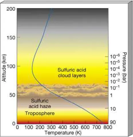
A scheme of Venus’s atmosphere is shown in Figure 3.
In terms of a detailed vertical structure of the Venus cloud system, the Cloud Particle Size Spectrometer (LCPS) on board the Pioneer Venus Sounder probe has provided excellent in situ measurements.
Figure 3. The probable structure of Venus’s atmosphere showing the main cloud layer and also how temperature (blue line) varies with height. The temperature scale is in K (kelvins) where 273 K = 0oC. [Graphic: NASA].
The actual amount of cloud droplets in the atmosphere is given by the mass loading of the atmosphere: the first 30 km are composed of clear CO2 air, with the thin haze extending upwards until the altitude where the
temperature drops to ~400 K and pressures of ~ 1 bar and the atmosphere is able to sustain H2S04 droplets. Then, between 44 and 48
km of altitude, a four orders of magnitude increase in the density of the cloud defines the beginning of the main cloud deck which extends upwards to 65 km altitude. Above that altitude, another haze layer spans a further 10 km. Vertical mixing from regions below the main cloud layer enriches it with sulphur dioxide and water. At the region of the cloud top a thin, but highly active photochemically layer exists and is the main
2.1.3 Winds on Venus
Unlike the Earth's lower atmosphere, which is mainly driven from bottom boundary by absorption of sunlight at the surface, Venus' atmospheric circulation is largely driven from above by the absorption of sunlight within and above the upper cloud layer. The cloud cover has an important influence on the atmospheric circulation by controlling the amount and distribution of solar energy absorption (Schubert, 1980).
One of the least explained phenomena of atmospheric circulation on Venus is its zonal retrograde super-rotation; the entire atmosphere, above the lowest scale height, extending upwards to >90-100 km, participates in the global super-rotation which was first observed in Earth-based ultraviolet pictures of the planet. The large-scale albedo feature known as the "dark horizontal Y" , visible in Figure 5, was observed to re-appear approximately every 4 Earth days, indicating a zonal rotation of the cloud level atmosphere with equatorial wind speeds of about 110 m s-l, which is
considerably faster than the rotation speed of the planet at the equator of 2 m s-l. This super-rotation is known to occur in the atmospheres of only
two solid body planets of our solar system, Venus and Saturn's largest moon, Titan. In the case of Venus the super-rotation is thought to reach the lower thermosphere, up to an altitude of around 100 km. At the cloud altitudes the wind speed and characteristics have been inferred from feature tracking in ultraviolet images of Mariner 10, Venera 9, Pioneer Venus and others. Above the clouds, in the absence of diagnostic features, analysis of Doppler shifts of selected molecular lines has provided further wind information. In Figure 4, averaged retrograde zonal wind velocities are shown as measured by experiments on board the Mariner 10 and Pioneer Venus satellites. The wind is maximum over the equator with speeds of ~100 m s-1 and drops off evenly towards the poles. The solid
curve represents the predicted zonal wind calculated for solid body retrograde rotation.
At the present date, the only large scale model describing the circulation of Venus' atmosphere is the Venus Thermosphere General Circulation Model (VTGCM) (Bougher et al., 1988). Further modeling is being prohibited by the inability to identify a suitable physical mechanism that explains the cloud-top super-rotation.
Figure 4. Longitudinally averaged retrograde zonal wind velocities vs latitude, inferred from tracking of small-scale cloud features from ultraviolet images of Venus. Triangles, Pioneer Venus, by Rossow et al. (1980); circles, Mariner 10, by Limaye and Suomi (1981); squares, Mariner 10, by Travis (1978). The solid curve is the zonal wind velocity calculated for solid body retrograde rotation with equatorial speed of 92.4 m s-l. Adapted from Schubert (1980).
2.2
Mars
In the last years Mars has been the target of most of the planetary missions. The huge amount of data collected by the spacecrafts has displayed a rich and diverse geological history, as well as many unsolved puzzles about the evolution of the planet and its present condition.
Although Mars is smaller than Earth (its radius is just a little over half of Earth's) it hosts a variety of impressive features: roughly along the equator there is Valles Marineris, a fault in the Martian crust 4000 km long (about a fifth of the distance around the whole of Mars), up to 600 km wide and 7 km deep; there is the Hellas Basin in the southern hemisphere , which is an enormous impact crater, 2300 km in diameter and more than 9 km deep; there is the highest volcano in the solar system, Olympus Mons which stands at 26 km above the surrounding plain; moreover Olympus Mons lies at the western edge of another impressive feature, the Tharsis region, which is a 10 km high, 4000 km wide bulge in the Martian surface. But probably the most intriguing issue about this planet is related to the role of water on its surface and the connected implications. Several of geomorphologic features (evidence of catastrophic floods, network of channels, layered rocks) let suppose that in the Martian past history water should have been stable on the planet surface. This implies that Mars was warmer and with a denser atmosphere in the past compared to the present conditions, making reasonable the exciting hypothesis that life could have developed in such kind of environment. At the moment the values of temperature and pressure at the surface are well below the triple point of H2O, making
impossible to have stable liquid water on the ground. Anyway the hypothesis that somewhere on the planet (under the surface or near some hydrothermal sources, if any) life could have developed and still
Other important characteristics of Mars are the presence of two polar caps that act as cold trap for CO2 and H2O, their seasonal regression and
condensation, a high (and highly variable) content of thin dust spread all over the planet that gives rise to several atmospheric phenomena such as dust storms (also at planetary global scale) and dust devils. Water vapor and water ice clouds are also present in the atmosphere.
The following pages provide a very short outline of our present knowledge of Mars, limited to the subjects more directly interested by IR spectroscopy investigation. An excellent review and historical introduction can be found in the volume Mars (edited by Kieffer et al., 1992) and reference therein. More recent results are mentioned explicitly along the text.
2.2.1 The Martian atmosphere: gaseous components
Table 5 lists the gases composing the Martian atmosphere, as measured by space probes.
The atmosphere is very thin: a reference, annual averaged, value for surface pressure can be set at 6 mbar. This value is extremely variable, due not only to the great topographic differences observed on the surface, but also because the temperature, during polar night, may fall below the condensation temperature of CO2, determining the frosting of a significant
fraction of atmosphere’s mass. This annual bimodal cycle was well observed by Viking landers (Figure 6).
The study of isotopic and elemental ratios has demonstrated that Mars experienced a substantial erosion of its primitive atmosphere, formed after the end of T Tauri phase of Sun’s life cycle. Different values have been proposed for the surface pressure of early Mars, but the orders of magnitude agree around one bar. Erosion affected mainly the carbon dioxide component, impact by meteoroids and thermal escape
representing the leading phenomena. Several authors pointed out the role of carbon inclusion in carbonates in a water-rich environment. Up to now, anyway, carbonates have not been detected on Mars and therefore this effect, even if present, should be of minor importance.
Constituent Volume mixing ratio
CO2 0.9532
N2 0.027
Noble gases (mainly 40Ar) 0.016
O2 0.0013
CO 0.0007
H2O 0.0003*
O3 0.2-0.04 ppm*
Table 5. Average composition of Martian atmosphere. Confirmed constituents only. *:average value, variable in time and space.
CO and O2 are both derived from CO2. The thinness of the atmosphere
and the (apparent) lack of a substantial ozonosphere allows to UV Solar photons to penetrate until the surface.
The photo-dissociation
2 CO2 + hν → 2 CO + O2 (0.1)
occurs therefore in the whole height of the atmosphere. The inverse reaction has a very low probability. In very simple conditions therefore, an enrichment of CO and O2 would be therefore expected.
Figure 6. Average daily pressure observed by Viking landers. Ls is the aerocentric longitude of the Sun, being 0 at the Northern spring equinox. This parameter is usually adopted to define the season. Upper curve: Viking lander 2; lower curve: Viking lander 1. Data from Tillman, J. E., 1989, PDS web site.
Predicted values exceed several order of magnitude the observed concentrations, demonstrating the existence of more complex mechanisms. Some catalytic cycles involving hydrogen have been proposed and, at this time, represent the more promising solution to the problem (see Atreya & Gu, 1995, for review). These reactions invoke also the production of quite exotic species such as H2O2 and some radicals,
but observative constraints in this sense are, at the moment, very sparse and basically limited to Earth observation. The situation is further complicated by reaction speed considerations related to the altitude. For CO and O2, as well as for the other atmospheric components but CO2, the
vertical mixing ratio profile remains almost unknown.
The role of water on Mars is the topic of much literature, probably exceeding any other subject in planetary sciences. H2O vapor presents a
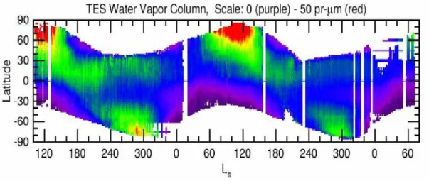
concentration very variable in space and time. Seasonal trends have been observed by MAWD and confirmed recently by TES instrument on MGS
(Smith M. D. et al., 2003a, Figure 7). Water vapor shows a maximum concentration during the retreat of the north polar cap, when an important fraction of H2O, trapped as ice during winter, is sublimated in
the atmosphere; another minor maximum is observed during southern spring.
Figure 7. Annual behavior of water vapor in the Martian atmosphere, as observed by TES instrument (from Smith M.D. et al., 2003a)
Soil plays a complex role as a water source/sink. External layers are important, due to their possibly hygroscopic character, on a seasonal as well as on a daily basis. Here, single water molecules are bounded by electric forces to polar sites of mineral crystals. Temperature of the soil drives the balance between released and captured molecules. Moreover, deep underground (i.e. some meters below surface) may possibly host the greatest planet water reservoir in form of permafrost, i.e.: water in a crystalline form dispersed in a matrix of mineral grains. Evidence of this sense is represented by rampart craters (Figure 8) as well as by observations of GRS experiment on Mars Odyssey (Boynton et al., 2002). Further details are being provided from MARSIS and SHARAD radar observations on Mars Express and Mars Reconnaissance Orbiter, but, at this time it is hard to quantify the total mass involved in these formations.
limited data is available up to now (Titov, 2002). Needless to say, the vertical distribution of water vapor is a particularly important subject because of the high number of atmospheric chemical reactions having H2O as a key player. Sky brightness observed at the Pathfinder site seems
to point toward a layer (with a thickness in the order of 1-3 km) with uniform mixing ratio close to the surface, overlaid by an almost dry atmosphere (Titov et al., 1999). Behavior of water vapor with height is constrained further by the observed distribution of ice clouds on Mars. The altitudes of these structures demonstrate how the vertical distribution of trace components of the atmosphere is influenced deeply by the great scale dynamic of the atmosphere (Rodin, 2002).
Figure 8. An example of rampart crater. Lobes at the rims of these structures are interpreted as evidences of the flow of a water-rich mud after the impact. The permafrost ice would have been liquefied by the heat released during the impact, giving to the ejecta mechanical characteristics very different from those of dry materials. (Images from MOC press release, August 13th,1998).
Liquid water cannot exist in stable form in today’s thin atmosphere. Several structures observed by spacecraft cameras on the surface demonstrated the existence of an ancient climatic regime very different
from the present one. Among them, channels systems and gullies appear particularly impressive (Figure 9). The dating of these structures in the context of Martian history is still a matter of debate, as well as the role of liquid water in the geochemical evolution of Martian surface (Hamilton et al., 2003, Wyatt & McSween, 2003). Ozone was detected by spacecraft UV observations in early ’70. Other measurements are available form Earth’s and HST observatories, as well as from the limited dataset of AUGUSTE experiment on Phobos 2 (Blamont & Chassefière, 1993). They are however too sparse to provide a clear picture of the temporal and spatial behaviors of this gas. Ozone is formed by photo - dissociation of O2, and subsequent
combination with another O2 molecule.
O2 + hν → 2 O (0.2)
O + O2 → O3 (0.3).
The process is inhibited by the presence of water vapor, which subtracts atomic oxygen, possibly in the context of the CO2-forming cycles. The
anti-correlation between O3 and H2O was confirmed by spacecraft
observations. The uncertainties about vertical distribution of atmospheric components do not allow ruling out an atmosphere of alternate water-rich and ozone-rich layers.
Other identified gas constituents have a minor importance. We mention only a nitrogen cycle, foreseen by models, but still without experimental evidence and little impact on global aeronomy of the planet.
For other gases, only upper limits have been fixed, mainly on the basis of IRIS data. Future experiments, namely PFS, will focus their attention on the detection of the species involved in the CO2 cycle and other minor
Figure 9. Channels systems (a.) and gullies (b.) have been invoked as proofs of the existence, in the past, of an environment able to sustain a complete water cycle on Mars. (Images from MOC press releases, June 22nd, 2000 and August, 8th, 2002)
2.2.2 Dust
Besides gases and water ice clouds, Martian atmosphere contains also an amount of mineral dust. Its presence results in several interesting phenomena. Among them, dust devils (columns of dust, with a diameter in the order of several meters and over 6 km high, raised from the surface by whirlpools, Cantor & Edgett, 2002), diffuse haze, and the impressive dust storms, that may hide wide areas of the surface from visual observations for several days.
The dust concentration in the atmosphere is extremely variable, and the observations of Viking landers have demonstrated that it can never be considered negligible. The optical thickness of the atmosphere decreases of only one order of magnitude from the peak of the greatest storm to the quietest periods (from 0.5 to 5, considering the visual region). Consequently, even if surface features can be observed in detail, great
care must be used in the analysis spectroscopic data, deformed in surface reflectivity features details as well as in the phase functions.
The first clues on dust composition come from early IRIS observation, acquired during the greatest dust storm ever recorded on Mars. The shape of thermal IR spectra is consistent with a silicate material, with moderate-high silica content. Moreover, dust must include some fraction of a magnetic material, as demonstrated by simple experiments on Pathfinder lander (Gunnlaugsson, 2000), probably represented by some form of iron oxide, as suggested by visual colorimetric studies. A more precise definition of dust composition has been attempted by several authors indicating montmorillonite + basalt, palagonite (Clancy et al., 1995) and a mixture of different materials, where albite (a member of feldspar group) represents the main constituent (Grassi & Formisano, 2000). None of these models are, at the date, able to reproduce correctly the observed spectra in all their details. Research in this field is still severely limited by the restricted availability of complex refractive indices of different geological materials.
Dust grains have a diameter in the order of micrometer, being therefore much smaller than usual Earth sand. The size distribution is anyway another point of discussion. Most recent results by Montmessin et al., 2002, point toward a bimodal function, indicating perhaps a variety of different phenomena at the origin of the aerosol. Analysis of temperature fields retrieved from IRIS data by Conrath et al. (1975) suggests a constant size distribution with height, despite the expected gravity-driven settling. The Clancy et al. 2002 study of a limited TES set of phase angle measurements claims, on the contrary, the actual occurrence of this phenomenon.
This picture of great uncertainty is completed by the considerations about the vertical distribution of dust. A general consensus grew around the Conrath et al., (1975) model, very similar to an exponential distribution. This measure is anyway a very indirect one. Sparse results by Phobos 2
Aerosol are known to be one of the key factors in the energy balance of the planet, and every aspect mentioned above, far from being a mere speculative interest, potentially has a great impact on their thermal properties, and, consequently, on our capability to model atmospheric phenomena. We shall also keep in mind that any study of spectral data aiming to retrieve surface or atmospheric properties, have the dust optical properties and size distribution as mandatory inputs. We will see that PFS does not represent an exception.
2.2.3 Main phenomena of Martian atmosphere
The study of Martian atmosphere’s dynamics is a subject of particular interest, due to the strong similarities with Earth. Moreover, due to very close values of the length of the day and inclination of rotation axes on the orbital planes, the two environments are characterized by similar boundary conditions. Being, for several aspects, a more simplified system, Mars study can provide very useful insights in the physics of air masses, that may possibly give us new prospectives and tools for the understanding of our own home planet.
Presently at least five global circulation models (Bridger, 2003) are available, being able to reproduce with reasonable accuracy the phenomena (temperature fields, winds, long-scale waves, pressure variations at the surface) observed by space instruments. This correspondence ensures us that main drive mechanisms of atmosphere dynamic have been considered in their relative importance. All these models anyway still present some weak points, where a parameterization of some complex process becomes needed. This means that the user is required to provide some input because the code is not able to foresee the situation by its own; very often these inputs are of key importance, as expected in an essential chaotic system such as an atmosphere. Examples