A real-time, GPU-based VR solution for simulating the POLYRETINA retinal neuroprosthesis

(1)

A real-time, GPU-based VR solution for

simulating the POLYRETINA retinal

neuroprosthesis

Candidato

Enrico Migliorini N. Matricola 880188

Relatore

Prof. Pier Luca Lanzi

Co-relatori

Prof.ssa Alessandra Pedrocchi Prof. Diego Ghezzi

(2)

(3)

Dedicated to my family, Jetsabel, Edoardo and Giulia, and in loving memory of Eleonora.

(4)

(5)

Date le moderne innovazioni nel campo della neuroprostetica, ossia la branca dell’ingegneria biomedica che si occupa di creare dispositivi per restituire facoltà motorie o sensoriali a pazienti affetti da disabilità, valutare l’efficacia e gli aspetti psicologici delle protesi è sempre più necessario. Poiché i ri-sultati di una tale valutazione sono estremamente utili per la progettazione delle protesi stesse, simulare i loro effetti fornisce facilmente dati preziosi.

Questo lavoro presenta il mio progetto di ideazione e realizzazione di un simulatore di visione prostetica, ovvero una combinazione di un ambiente virtuale e una serie di filtri che permettano ad una persona vedente di vedere l’ambiente come lo vedrebbe una persona non vedente cui sia stata impiantata una specifica protesi retinica, vale a dire un dispositivo che restituisca in parte le facoltà visive perse a causa di lesioni della retina.

Questa tesi inizia col dare una panoramica delle protesi retiniche e della realtà virtuale, descrivendo la loro storia, lo stato dell’arte e le opportunità che offrono. Il capitolo 3 descrive l’infrastrattura hardware usata, mentre il capitolo 4 espone nel dettaglio il funzionamento del simulatore ed il capitolo 5 descrive i protocolli dei test. Infine, il capitolo 6 discute i risultati e i possibili sviluppi futuri.

Le appendici includono frammenti di codice nell’appendice A e i risultati sperimentali del test nell’appendice B.

(6)

(7)

Sommario I

Table of Contents III

List of Figures IV

List of Tables VII

List of Abbreviations VIII

1 Introduction 1

1.1 Aim of the project . . . 1

1.2 Proposed approach . . . 4

1.3 Outline . . . 5

2 Background 6 2.1 Retinal prostheses . . . 6

2.1.1 Retina-based loss of vision . . . 6

2.1.2 Retinal prostheses . . . 8

2.1.3 The idea behind POLYRETINA . . . 13

2.1.4 Layouts of POLYRETINA . . . 14

(8)

2.2.1 History and basic principles . . . 15

2.2.2 The use of Virtual Reality in sensory neuroprosthetics . 17 3 Hardware setup 20 3.1 The visor . . . 20

3.2 The Motion Capture system . . . 22

4 The Simulator of Prosthetic Vision 24 4.1 State of the Art . . . 24

4.2 Reason for using a GPU . . . 25

4.3 Shaders . . . 26

4.3.1 Pre-processing . . . 28

4.3.2 Stimulation pattern . . . 31

4.4 The test environment . . . 38

5 Tests 40 5.1 Test 1: Object recognition . . . 40

5.2 Test 2: Reading single words . . . 42

5.3 Test 3a: Finding objects in an environment . . . 44

5.4 Test 3b: Motion Capture integration . . . 46

5.5 The test subjects . . . 47

6 Conclusions and discussion 48 6.1 Overall results . . . 48

6.2 Future developments . . . 50

Appendices 52 A Code fragments . . . 53

(9)

1.1 Function of a visual prosthesis . . . 2

1.2 The SPV applied to the images supplied by a camera . . . 3

1.3 How the electrodes were translated to points. . . 4

2.1 The retina and its two most common dystrophies . . . 7

2.2 A cortical prosthesis. From [Li, 2013]. . . 10

2.3 A retinal prosthesis. From [Beyeler et al., 2017]. . . 11

2.4 The Argus R _{II Retinal Prosthesis System . . . .} ₁₂

2.5 The first prototype for POLYRETINA. . . 13

2.6 Layouts of POLYRETINA . . . 14

2.7 Virtual Reality devices through the ages . . . 16

2.8 A surgeon uses VR to explore a 3D reconstruction of his pa-tient’s brain . . . 18

3.1 The FOVE HMD . . . 21

3.2 The motion capture setup in action . . . 23

4.1 An image, before and after the shader described above was applied . . . 28

4.2 Edge detection . . . 30

4.3 Different techniques for digitally reproducing phosphenes. From [C.Chen et al., 2009]. . . 31

(10)

4.4 References to find the closest pixel. . . 34 4.5 The data object for an 80/120, 46.3◦layout, visualized as a

texture . . . 36 4.6 The image after post-processing . . . 38 4.7 One of the virtual environments as experienced by the users . 39 5.1 Examples from Test 1 . . . 41 5.2 Examples from Test 2 . . . 43 5.3 The room’s layout . . . 44

(11)

2.1 Number of pixels per different values of pitch . . . 15

5.1 Test Subjects . . . 47

6.1 Calculated visual acuity . . . 49

B.1 Test 1 - Accuracy (Noise/No Noise) . . . 66

B.2 Test 1 - Accuracy (First/Second Time) . . . 66

B.3 Test 1 - Times (Noise/No Noise) . . . 67

B.4 Test 1 - Times (First/Second Time) . . . 67

B.5 Test 2 - Accuracy . . . 68

B.6 Test 2 - Accuracy (effect of the angle for different layouts) . . 69

B.7 Test 2 - Accuracy (effect of the layout for different angles) . . 70

B.8 Test 2 - Times . . . 71

B.9 Test 2 - Times (effect of the angle for different layouts) . . . . 71

B.10 Test 2 - Times (effect of the layout for different angles) . . . . 72

B.11 Test 3a - Times . . . 73

B.12 Test 3a - Average time values . . . 74

B.13 Test 3a - Times (considering the iteration) . . . 74

B.14 Test 3b - Times . . . 75

(12)

CPU Central Processing Unit DSE Design Space Exploration GPU Graphics Processing Unit

HMD Head Mounted Display

MEA MicroElectrode Array

SIMD Single Instruction, Multiple Data SPV Simulated Prosthetic Vision VPU Vision Processing Unit

(13)

(14)

Introduction

This thesis exposes my Masters’ Thesis project, aimed at developing a Virtual Reality framework for testing different configurations of a neuropros-thetic device being developed at the LNE lab, in EPFL.

1.1 Aim of the project

Visual neuroprostheses are devices that are built to interface with the hu-man nervous system and partially restore visual faculties in visually-impaired subjects.

Although the base concept was first proposed in 1929 [Förster, 1929], it’s only in the last decade that a design able to restore a modicum of visual capabilities, the Argus R _{II has been approved as a medical device outside}

the scope of research, and is now available to the public [Luo et al., 2014]. One reason for the long time it took to release a device to the public was the lengthy process that implantable devices have to go through before they are fit for human testing. As with all engineering projects, the creation of a retinal prosthesis needs to go through a loop of planning, designing, testing

(15)

Figure 1.1: Function of a visual prosthesis

and evaluating before it is fit for release: but since the time investment required for actual testing is gargantuan, the time scale of the project dilates proportionally.

There are, however, tools that can be used to assist prototyping, so that an initial phase of testing can start at the same time as prototyping. Those tools allow to perform Design Space Exploration (DSE), that is the analysis and evaluation of a range of designs by using simulations, rather than actually manufacturing the devices. DSE is usually applied to electronic and embed-ded systems, where a wide range of metrics can be applied to evaluate the performance of a design, but for testing a device such as a prosthesis, where subjective experience is paramount, a modified approach must be adopted.

(16)

This thesis project used Virtual Reality (VR) environment to create a perceptual experience by the name of Simulation of Prosthetic Vision: that is, a combination of a virtual environment and a series of filters that allow a sighted person to experience the world as seen through the eyes of someone implanted with a specific device developed to alleviate blindness.

Figure 1.2: The SPV applied to the images supplied by a camera

Through the use of the SPV, it is possible to simulate a wide range of devices, with widely different specifications. This work focused on POLY-RETINA, a retinal prosthesis (that is, one which stimulates the retina dir-ectly through electrodes, more about that in Section 2.1) being developed in the LNE laboratory of EPFL. Different configurations of POLYRETINA could be tested and evaluated, allowing precious insights over which configur-ations were the most cost-effective, how much of an improvement this device would be from the current state of the art, and how much different fields of view impacted the overall device effectiveness.

(17)

1.2 Proposed approach

The first step to create a simulation of prosthetic vision was to find a mathematical model that would transform a picture into a pattern, apply-ing post-processapply-ing algorithms and what we know about retinal stimulation to generate a heavily degraded image, as close as possible to the reported perception of a patient implanted with the actual device.

This resulted in a honeycomb pattern of blurred dots. This is because the literature review showed how the stimulation of the retina by an electrode results in the perception of a bright dot of light with blurred edges. As such, the electrodes present on the surface of POLYRETINA were mapped 1-to-1 to areas in the visual field. Wherever an electrode was supposed to be activated, a white dot was shown, and the rest of the visual field was set to black.

(a) The electrodes in POLYRETINA

(b) The simulated electrode pattern

(c) The resulting phosphenes

Figure 1.3: How the electrodes were translated to points.

This pattern was then shown to the subject through the use of a VR Head Mounted Display (HMD). This allowed the subject to experience an immersive simulation, perceiving the environment as a subject implanted with a given configuration of POLYRETINA would. Additionally, the eyes were tracked, allowing the subject to experience different parts of their sur-roundings just by moving their eyes.

(18)

Once the model was created, four different tests were run on sighted volunteers, measuring how accurately and how quickly they could take in details of the virtual environment. These tests ranged from identification of objects and words to full movement and exploration of a virtual environment such as a room. They were performed on members of the LNE laboratory, in the facilities of the Fondation Campus Biotech Geneva, located in Geneva, Switzerland.

These tests were aimed at finding out which configurations offered the best value, especially considering the effort, cost and difficulty of manufacturing them. To that result, extensive statistical validation was then performed on the collected data.

1.3 Outline

This work will start with an overview of retinal prostheses and Virtual Reality, describing their history, state of the art and the opportunities that they present. Chapters 3 and 4 will describe the hardware tools used to cre-ate the SPV and the actual algorithms, while 5 describe the test protocols. Finally, Chapter 6 will discuss the results and the possible future develop-ments of the work. The actual results and statistical analysis of the tests can be found in appendix B. While interesting in its own regard, the actual effectiveness of the prosthetic device is out of the scope of this thesis.

(19)

Background

This chapter provides a background into retinal prostheses and Virtual Reality, the two overarching concepts that are integrated in this project. It briefly explains their basic principles of functioning and touches some historical notes. Additionally, it presents POLYRETINA, a novel retinal prosthetic device and the focus of this project.

2.1 Retinal prostheses

2.1.1 Retina-based loss of vision

The retina is a light-sensitive tissue located at the back of the eye (see Figure 2.1a), which is responsible for converting ambient light into electrical signals, which are then sent to the visual cortex via the optic nerve. As such, it is a central and essential component of vision: retinal dystrophies, such as retinitis pigmentosa or age-related macular degeneration, can drastically impair vision, leading to blindness.

The retina works thanks to two highly specialized kinds of neural cells, rods and cones. These cells are photoreceptors, which means that they send

(20)

(a) Section of the eye (b) A healthy retina

(c) A retina affected by retinitis pigmentosa

(d) A retina affected by macular degeneration

Figure 2.1: The retina and its two most common dystrophies

an electrical signal when they are hit by light at certain frequencies. Rods are sensitive to a wide specter of wavelengths and have a lower threshold for activation, but can’t differentiate between colors: they are responsible for our night vision. Cones, on the other hand, exist in three variants, depending on whether they are sensitive to the red, green or blue color. The signals sent by the photoreceptor cells are then sent to the gangliar cells, neurons whose axon form the optic nerve. From there, the signal is sent to the visual cortex,

(21)

an area of the cerebral cortex situated towards the back of the brain, which processes it to create the perception of vision [Gartner, 2016].

Retinitis pigmentosa is a genetic disorder causing gradual damage to the photoreceptors, eventually leading to blindness over the course of several decades. It affects approximately one person every 4000 [Hamel, 2006]. As for age-related macular degeneration, it is a condition leading the patient to lose vision in the center of their retina. Although it does not lead to total blindness, it severely impairs one’s ability to recognize objects, read or perform other daily tasks. It is the leading causes of irreversible blindness in adults over 50, and there is no known cure [Pennington and DeAngelis, 2016]. The overall prevalence is 8.69%, although it varies greatly among different ethnicities [Won et al., 2014].

2.1.2 Retinal prostheses

As with cochlear implants allowing deaf people to hear, so technology is coming to help alleviate blindness, and allow those affected by retinal degeneration to lead normal lives through the use of prosthetic devices. These devices take the place of the damaged organ or tissue (in this case the retina), artificially converting the trigger (light signals) into electric signals for the brain. That is done via the use of electrodes, which can stimulate neurons with electrical impulses.

There are currently two main categories of prostheses intended for the visual pathways: retinal and cortical ones. The working principle is the same: pictures are captured by a camera and pass through a Vision Processing Unit (VPU). This is a computing device that converts the picture into an activation pattern and sends it to implanted electrodes, which stimulate the underlying neural cells.

(22)

As has been known since 1929 [Förster, 1929], when electrodes deliver an electrical impulse to the underlying neuronal tissue, they generate the perception of light, what is called a phosphene. From reports of patients who have been implanted with retinal neuroprostheses, the perceprion of a phosphene is that of a roughly circular spot of light in their field of vision, in a location according to their placement on the retina. The mapping between the stimuli and the perception, i.e. the mapping of the visual field to retinal neurons, allows us to calculate and reproduce what the user will perceive from a given stimulus. For instance, we know that the image projected on the retina is flipped: therefore, a stimulation to the lower half of the tissue will result in a perceived phosphene in the upper half of the visual field [Tassicker, 1956].

Cortical prostheses, improving on the basic concept found in [Förster, 1929], bypass the eye in its entirety: they are applied directly to the brain’s visual cortex, creating phosphenes (a phosphene is a sensation of bright light) in the corresponding portion of the visual field. The pattern is generated tak-ing into account the mapptak-ing of the retinal visual field with the correspondtak-ing areas of the visual cortex, what is called a retinotopic mapping [McLaughlin et al., 2003].

The main advantage of cortical implants is that they can be used to alleviate a wide variety of visual impairments: as they bypass all of the eye and the optic nerve, they can be used in cases of lesions that do not affect the retina itself. However, the disadvantages are significant: they require intra-skull surgery to be implanted, and the current limits of technology and the anatomical structure of the cortex itself create a harsh upper bound for the number of electrodes that can be placed in an area before cross-electrode interactions and medical safety concerns become an issue [Li, 2013].

(23)

Figure 2.2: A cortical prosthesis. From [Li, 2013].

Retinal prostheses, on the other hand, interact with the retina itself, bypassing the damaged layer of photoreceptor cells and instead stimulating directly the gangliar cells. The idea behind these devices was formulated in 1956 [Tassicker, 1956], with a working prototype developed in 1968 [Brindley and Lewin, 1968]. These devices can be either epiretinal, if they are placed on the retinal surface, or subretinal if they are under it. This distinction also influences how the electrodes are designed to function.

Epiretinal prostheses are realized by implanting a microelectrode array (MEA) connected to a small signal processor through a ribbon cable. The ac-tivation pattern is sent to the signal processor, which activates the electrodes accordingly. The one displayed in Figure 2.3 is an epiretinal prosthesis. An example of epiretinal prosthesis is described in detail later in the chapter.

Subretinal prostheses, on the other hand, use photodiodes, stimulating the gangliar cells according to the ambient light that is entering the eye through the pupil. This removes the need for cameras, however invasive surgery is still required: the diodes do not generate a strong enough voltage to activate neurons, so they require amplifiers which are externally powered

(24)

Figure 2.3: A retinal prosthesis. From [Beyeler et al., 2017].

via a cable connected to a battery via an induction coil. An example of subretinal prosthesis was the alpha-IMS implant [Stingl et al., 2013], whose development was interrupted in 2016.

When compared to cortical prostheses, retinal prostheses have the ad-vancement of being less invasive and the potential for a higher number of electrodes, resulting potentially in a wider field of view or a higher resolu-tion. Additionally, there is no need to consider the retinotopic mapping of retinal neurons to the visual cortex, so the perceived image will have a lower amount of spatial noise.

In order to make more clear how POLYRETINA innovates, here is presen-ted a different, currently state-of-the-art MEA-based epiretinal prosthesis: the Argus R _{II Retinal Prosthesis System, developed by Second Sight}

Med-ical Products [Luo and da Cruz, 2015] and the first retinal prosthesis to be approved by the United States Food and Drugs Administration (FDA). The Argus R _{II records images from the surrounding environment, processes them}

(25)

via an integrated system, then sends the activation pattern to an array of 60 electrodes via a transmission coil. These electrodes need to be powered by an external energy source, therefore the device also includes a portable battery.

(a) The internal components (b) The external components

Figure 2.4: The Argus R _{II Retinal Prosthesis System}

The low amount of electrodes, due to the space needed for wiring and the risk of overheating damage, means that the resolution of such a device is extremely low: the visual acuity of an Argus R _{II prosthesis is 20/1262, where}

blindness is defined, in North America and most of Europe, as visual acuity of 20/200 or lower, or a visual field no greater that 20 degrees [United States Code, 1986], and as a visual acuity of 20/400 or lower by the World Health Organization. Not only is the resolution of the Argus R _{II low, its field of view}

is also limited: the Surgeon Manual for the device states that it is designed to offer "a visual field of 9 by 16.5 centimeters at arm’s length" [Argus R _II

Surgeon Manual, 2013], or an angle of approximately 17◦. Again, that result falls under the legal requirement for blindness.

As of 2019, no retinal prosthesis model has managed to reach an estimated visual acuity even approaching the threshold of legal blindness. This is why POLYRETINA [Ferlauto et al., 2018] is being developed, as a high-resolution,

(26)

wide-angle prosthetic device able to cross the blindness threshold, and to allow patients to lead normal lives.

2.1.3 The idea behind POLYRETINA

Polyretina is a foldable, wide-field epiretinal prosthesis, designed to com-bine the advantages of epiretinal and subretinal prostheses: photovoltaic stimulating pixels are bonded to a semiconductor layer and a top cathode in titanium (Ti). Each of these pixels activates when illuminated by a strong enough light, stimulating the underlying gangliar cells and resulting in a phosphene.

Figure 2.5: The first prototype for POLYRETINA.

The use of photovoltaic electrodes means that no wiring is required: the pixels are activated by pulsating light on them with a small projector, and no battery is needed since the energy required to activate the electrodes is obtained by the light itself. The lack of wires allows a considerably larger numbers of electrodes to be placed on the device, so that the implant can cover a wide field of view without sacrificing resolution. Additionally, the

(27)

device is also less invasive than the current prototypes: although surgery is still required for the implant, there are no cables connecting it to the outside, and not having power cables means that the heat generated by the device will be low enough to avoid overheating issues.

2.1.4 Layouts of POLYRETINA

The layout of POLYRETINA as described in [Ferlauto et al., 2018], com-posed of a circle, a ring and a number of clusters in the periphery, was later discarded for a single circle, where electrodes are arranged in a honeycomb pattern. The circle has a 13 mm diameter, factoring an increase due to radial elongation when the disc is shaped into a spherical cap. Considering that the distance of the retina from the focal point is 17 mm, this results in a field of view of 46.3 degrees.

(a) The first prototype (b) The model being developed

Figure 2.6: Layouts of POLYRETINA

Once the area to be covered by the electrodes has been defined, the layout of a model is identified by two parameters related to the electrodes: diameter and pitch. The first is self-explanatory, while the second refers to the distance between the centers of two adjacent electrodes. For an example, the inner

(28)

circle of the prototype was made of electrodes of 80 µm , each distant 150 µm from its neighbours.

The amount of electrodes present in each layout is a function of the pitch: the smaller it is (obviously, it cannot be equal or lower than the diameter) the more electrodes can be placed on its surface. Experimental data and calculations tell us the number of pixels that can fit on the surface of POLY-RETINA.

Table 2.1: Number of pixels per different values of pitch Pitch Pixels

150 6717

120 10499

90 18693

60 42235

These numbers are far higher than the amount of electrodes for currently state-of-the-art prosthetic devices, like the 60 in the Argus R

II device.

2.2 Virtual Reality

2.2.1 History and basic principles

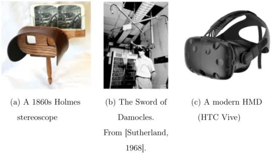
The term Virtual Reality (VR) refers to the process of simulating an immersive world through the use of technology, and presenting it to the user in such a way to make them suspend disbelief and accept the simulated perceptions as their own. Simulating visual experiences is a relatively old concept: the stereoscope was a popular tool in the 19th century to experience photographic images with the illusion of depth. They worked by taking two

(29)

slightly different pictures of the same scene with two cameras separated by a distance equal to the one between human eyes, then printing those photos side-by-side. The stereoscope, through the use of lenses allowing the eye to easily focus on the images despite their proximity to the eye, would then present each picture to the corresponding eye. This recreates the way that our brain perceives the world, since what gives us natural depth perception is how our eyes see objects from slightly separate points of view.

The modern idea of creating immersive Virtual Reality environment via the use of computers can be traced to Ivan Sutherland, computer scientist and pioneer in the field of computer graphics, who first suggested, in his 1965 article The Ultimate Display [Sutherland, 1965] the possibility of displaying images which would change according to the user looking at different points in space. Sutherland went ahead to building what is likely the first computerized VR head-mounted display (HMD), a large device nicknamed the Sword of Damocles [Sutherland, 1968]. (a) A 1860s Holmes stereoscope (b) The Sword of Damocles. From [Sutherland, 1968]. (c) A modern HMD (HTC Vive)

(30)

The Sword of Damocles sent sthereoscopic wireframe images to mini-ature cathode ray displays placed over the eyes of the user, and tracked head movements via a ultrasonic head position monitor. Despite the technolo-gical limits of the 1960s’ computers, the device managed to give the illusion of three-dimensionality, and allowed users to examine the presented images from a variety of points of view.

Modern VR HMDs are more compact, portable and have a higher resol-ution, but the basic working principle is the same: stereoscopic images are projected on a display, and when looked at through lenses, the users can visually experience a computer-generated world.

VR devices have a variety of uses in the modern world. They have recently become widely popular in the entertainment business, especially for computer games, but that is far from their only use: VR solutions have been developed for guiding drones (unmanned vehicles) [Smolyanskiy and Gonzalez-Franco, 2017], presenting 3D models of products to be developed, assisting with edu-cation [Freina and Ott, 2015] and even operating fine machinery like surgical robots [Khor et al., 2016]. VR has also proven to have a variety of med-ical applications, from the treatment of anxiety and other mental health is-sues [Valmaggia et al., 2016] to helping cope with pain [Dascal et al., 2017] to assisting in rehabilitation after traumatic brain injuries [Dascal et al., 2017] to detecting, via functional Magnetic Resonance Image (fMRI) how brain activity changes in different virtual environments [Adamovich et al., 2009].

2.2.2 The use of Virtual Reality in sensory

neuropros-thetics

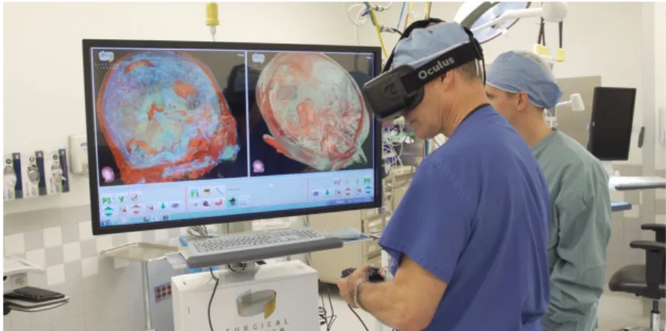
The technical, psychological and behavioral aspects of seeing through a prosthetic device are of the utmost interest to researchers in

(31)

neuroprosthet-Figure 2.8: A surgeon uses VR to explore a 3D reconstruction of his patient’s brain

ics. Due to the stringent regulations and the extended times required for performing human testing, a need has arisen to allow researchers to explore the implications of prosthetic vision via experiments performed on sighted subjects. That is possible by artificially simulating the visual perceptions be-lieved to be experienced by patients implanted with the device in question. This process is known as Simulation of Prosthetic Vision(SPV).

The first SPV tool was developed shortly after the first retinal pros-theses [Sterling et al., 1971]. The technology used at the time was rather crude: for the next three decades, SPV tools consisted mostly in monitors covered by perforated film, so that the subjects would experience only a cer-tain number of pixels of the image [Cha et al., 1992b]. The advent of modern, inexpensive Virtual Reality devices provided a new, powerful tool for SPV: image processing algorithms can be easily applied to VR visual output, al-lowing the user to experience the world as a patient implanted with a certain device would.

Literature already presents several experiments using SPV to evaluate prosthetic devices: they have been used for testing performance when reading

(32)

[Dagnelie et al., 2006a], hand-eye coordination [Dagnelie et al., 2006b], object tracking [Hallum et al., 2005] and mobility through a maze [Cha et al., 1992a]. The main aim of this thesis project was to examine in detail how the increased resolution an visual angle of POLYRETINA would affect accuracy and speed on several visual tests when compared to state-of-the-art results, with the further goal of determining which one was more cost-effective (as manufacturing smaller electrodes is significantly more expensive and diffi-cult). SPV proved to be the perfect tool for this kind of Design Space Ex-ploration (DSE): a procedurally generated computer simulation based on the desired resolution and targeted visual angle allows to test the effectiveness of various configurations, bypassing the expensive and time-consuming process of manufacturing the devices and going through animal and human testing. There are a number of decisions to be taken and challenges to be overcome when designing an SPV, however [C.Chen et al., 2009]: overly simplistic al-gorithms, or ones that are not solidly grounded in descriptions provided by first-hand observers (that is, reports by human subjects implanted with sim-ilar prostheses) would produce erroneous and misleading results. Therefore, special care was taken during the design to make sure that the simulated phosphenes were accurate in shape and position.

In the next chapter the technical details about the SPV developed during this project will be presented and explained.

(33)

Hardware setup

This chapter focuses on the hardware tools that were used during the process. It will introduce their functioning and present how they were used during development of the SPV.

3.1 The visor

The visor chosen to perform the testing was the FOVE 0 1. The FOVE has a 70-Hz, 2560x1440 display and the usual suite of accelerometers and gyroscopes which allow head tracking, but most importantly it includes two low-latency eye trackers.

Eye tracking is a technology that allows a computer to trace where a subject is looking. This is vital for simulating a retinal prosthesis such as POLYRETINA: as the electrodes do not cover the entirety of the retina, a subject cannot observe their surroundings in their entirety, but is limited to a circular area: the angle formed by two diametrically opposed points on this area’s border and the center of the retina is the visual field of the prosthesis.

(34)

Since POLYRETINA is affixed to the eye, it moves with it: this will allow a patient who has been implanted the device to see different portions of the surrounding environment just by moving their eyes, without needing to move their head as well.

Figure 3.1: The FOVE HMD

It follows that the visual field has to move on the VR visor’s screen accord-ing to eye movements, in order to allow a simulation subject to effortlessly explore their environment. Eye tracking is the simplest, least invasive way to allow subjects to move the phosphene field that makes up their perception to different locations in their field of view.

Eye tracking works by projecting near-infrared light on the eyes of the subject, then studying the reflection patterns on the iris. These patterns are dependent on the position of the pupil, therefore simple 3D geometry can output a vector that will reveal the direction of the viewer’s gaze. When

(35)

crossing this vector with the plane that is the actual display of the HMD, we obtain screen coordinates that will be used as the center of the visual field.

3.2 The Motion Capture system

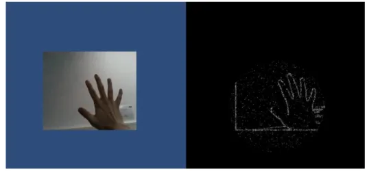
As will be explained in more detail in 5.4, one of the tests required subjects to explore a virtual reality environment. In order to navigate it, it was necessary to allow the subject to move freely, observing their surroundings from different perspectives. Having the subject control their avatars via a controller or other interfaces would have resulted in motion sickness, due to the perceptions from the eyes not lining up with the feedback from the vestibular system [Hettinger and Riccio, 1992].

One method that is occasionally used to counteract VR sickness is al-lowing the user to teleport their avatar in a different location, doing away with the illusion of motion. Such a system, however, was impractical for our needs: in order to be used effectively, it requires the subject to have a good spatial awareness of the virtual environment, something we were testing for. The solution we adopted was the use of an OptiTrackTM Motion Capture system: such a system is made of 15 infrared cameras capturing images from a 4m x 4m room from different points of view. Reflective markers arranged in pre-determined patterns are placed on the subject’s head and hands: from the images captured by the cameras, 3D reconstruction algorithms can provide a computer program with the subject’s 3D coordinates. Therefore the subject can simply walk across the room, and their movements will be related to the VR avatar. As the images then move according to the subject’s head movements, vestibular and visual feedback act in concert, removing motion sickness. Similar technology is used by the VIVE Lighthouse system in order

(36)

to provide low-latency position tracking and improve user experience [Nie-horster et al., 2017].

None of the subjects reported motion sickness during the test.

Figure 3.2: The motion capture setup in action

In the next chapter, I will present in detail the algorithm I created. I will compare it to the state of the art and describe its working principles in detail.

(37)

The Simulator of Prosthetic

Vision

In this chapter I provide a detailed explanation of how the simulator works.

4.1 State of the Art

Previous SPVs in literature were unusable for testing POLYRETINA, as none of those algorithms could handle the amount of data required to run a real-time VR simulator with such a high electrode count. This is because state-of-the-art SPVs either handled a significantly lower number of elec-trodes (e.g. [Shanquing Cai et al., 2005], [Cha et al., 1992a] and [Dagnelie et al., 2007]), used static images ( [Dagnelie et al., 2006a], [Jason A. Dowl-ing, 2004]) or were simply not aimed at providing a real-time simulation ( [Beyeler et al., 2017]). The pulse2percept open-source framework stands out as an eminent example: in order to simulate the Argus R II prosthesis for

(38)

factors of an algorithm relying on the operation of convolution to generate the stimulation pattern, and especially the fact that pulse2percept is built to run on a Central Processing Unit (CPU), instead of a Graphics Processing Unit (GPU).

Looking at the state of the art, the only article mentioning an architecture other than a CPU is Eckmiller [Eckmiller et al., 2005], who used a Digital Signal Processor to run a simulation of just 256 pixels. One of the main aims of this project was to show how the use of algorithms thought for usage on GPU could result in a simulator that was fast enough to render in real time an unprecedented number of electrodes. This meant moving away from the convolution-based state-of-the-art ones, and instead developing novel ones to take advantage of the massive parallelism of graphic cards.

4.2 Reason for using a GPU

A CPU is the core of a computer, an unit made of a relatively small processors (usually 2 to 32) which handles all the processes running on the machine. CPUs are built to take complex scheduling decisions, dedicating processing resources to different tasks and switching on the fly depending on the requirements of the system. However, the limited number and high cost of processors means that CPUs have a very low degree of parallelism, only managing to handle a limited number of operations at a time. This means that they are good at handling programs with a complex data flow, loops and branches, but they fall short on operations that need to be run on a large amount of data at the same time, such as image processing.

GPUs, on the other hand, are built to use a large amount of simpler, and relatively inexpensive cores. They do not handle complex branching

(39)

and scheduling as well as CPU cores, but they allow for a massive amount of parallelism. For example, the nVidia GeForce GTX 1080Ti, which was used to run Test 3b, has 3584 cores, all able to process data at the same time. This makes GPUs exceptionally suited at running Single Instruction, Multiple Data (SIMD) programs, where a single program is run over a large array of data. This, as their name implies, means that GPUs are uniquely suited to graphic tasks, where rather simple algorithms are applied to every pixel on screen.

The large number of electrodes of POLYRETINA, coupled with the need for a real-time simulator which can run at a high framerate (which is required in order to minimize VR sickness [Hettinger and Riccio, 1992]) means that a large amount of information must be processed in a few milliseconds: even at the lowest resolution of POLYRETINA, the effects of 6717 electrodes need to be applied over a 2560x1440 display. There is no way that any CPU currently on the market can achieve such a high throughput.

Therefore, it was needed to create a novel SPV, which could exploit the GPU’s high degree of parallelism to deliver the visual input with the shortest possible delay. This, however, requires a different algorithm than the ones currently in use with CPUs: that is because GPU programming has some significant differences from CPU programming.

4.3 Shaders

A shader is a program that runs on the computer’s GPU. When the CPU instructs the GPU to render a scene, i.e. turning information about the scene into an image, the GPU runs the shaders in order to generate additional data, which will be used to render the final image. Although their original use was

(40)

(as the name suggests) to produce appropriate levels of light, darkness and shadows in an image, shaders nowadays can be used to achieve a variety of effects: they can make surfaces look metallic and reflective, generate complex light effects, add distortion, act on brightness, contrast and color profile.

There are two kinds of shaders. The first kind is the vertex shader, which is applied to the vertices of any polygon making up the scene’s meshes (i.e. the objects on screen). Vertex shaders are used, for instance, to calculate the incidence and direction of light for reflections, and to determine whether certain surfaces are visible or hidden.

The second kind is the fragment shader, which is applied to every pixel in the scene. Fragment shaders can be used to add many kinds of image effects to a picture: for example,

f l o a t 4 frag ( v 2 f _ i m g i ) : C O L O R {

f l o a t 4 r e s u l t = t e x 2 D ( _MainTex , i . uv ); r e s u l t . r = 1.0;

r e t u r n r e s u l t ; }

is a small fragment shader (note that several declarations and compiler dir-ectives have been excluded for the sake of brevity) which sets the red channel of every pixel to 1 (maximum). The effect of this shader is shown in Figure 4.1.

Two fragment shaders made up the backbone of the SPV developed for this project. The first would take on the role of the external image processor: it applied enhancement algorithms to generate the picture that, in a com-plete POLYRETINA prototype, would then be projected onto the patient’s retina. The second one was the SPV proper: starting from the image output by the pre-processing shader, it created the honeycomb phosphene pattern

(41)

(a) The base image (b) The shaded image

Figure 4.1: An image, before and after the shader described above was applied

corresponding to the perceptual experience of a POLYRETINA user. The decision to use shaders and the design of the actual GPU algorithms mark the biggest improvement from the state of the art, as mentioned above. While image processing dove via a CPU can access straightforwardly different parts of the image at once, by default a fragment shader can only refer to the pixel it is currently elaborating. It is possible to access other portions of the image via an operation called texture sampling, but that is an expensive function, better to be used sparingly.

4.3.1 Pre-processing

If the stimulation pattern were to be generated directly from the virtual environment (applying a luminance-based threshold to decide whether an electrode is activated or not) it would be impossible to make out objects against a background of comparable brightness. Therefore, an edge detection algorithm is applied to the image.

(42)

The algorithm consists of three operations: first, a gaussian blur is applied to the image. This reduces the false positives due to image noise and artifacts, and allows an edge to be detected where a sharp contrast is present.

Afterwards, the Sobel operator [Sobel, 2014] is applied. This operator uses a pair of 3x3 matrices as convolution kernels over the blurred image.

The two matrices are

Gx =      −1 0 +1 −2 0 +2 −1 0 +1      and Gy =      −1 −2 −1 0 0 0 +1 +2 +1     

where the former detects horizontal gradients and the latter detects vertical ones. Subsequently every pixel’s RGB channels are set to the maximum value among them, turning the image into grayscale. Every pixel’s white value (that is, the RGB channels are set to the same number: a white value of 0.0 means that the pixel is black, 1.0 means it is white) is then set to q

G2_x+ G2_y.

The final step of the algorithm is edge enhancing: where usually edge detection algorithms try to make the edge as thin as possible, for the purposes of the test a thicker edge was more useful. This is because a thin edge is not bright enough to activate the electrode, and in simulation terms it would have been more unlikely for the pixels’ centers to precisely overlap with one of the edges. That would have resulted in a mostly black picture. This is done by setting every pixel’s white value to the maximum value in a 5-pixel radius circle around it, and setting the gray pixels which are closest to a darker area to white, to strengthen weak edges.

The output of the algorithm can be seen in Figure 4.2.

The greatest challenges during the creation of this shader consisted in the choice of algorithms: edge detection algorithms are plentiful, each working

(43)

(a) The base image (b) The image after edge detection

Figure 4.2: Edge detection

better for different kinds of pictures. The whole process is similar to the Canny edge detector [Canny, 1986], a well-studied algorithm. Despite being sensitive to some kinds of noise when detecting weak edges (small changes in contrast), the Canny algorithm places a light computational load on the computer [Wang and Fan, 2009]. The fact that weak edges are ignored by the Canny algorithm can also benefit us in this specific project: when looking at a picture with many small changes in color, as a carpet or a grass field could be, a more accurate algorithm would detect a noisy mass of white edges.

Edge enhancing was an original addition, inspired by similar researches such as [Luo et al., 2014], where black cardboard cut-outs were placed on the objects to be identified. That gave me the idea to increase the contrast to a very high value and making sure that the edges would remain visible throughout the small, involuntary head and eye movements. The desired thickness of the edges was determined through trial-and-error, looking for a value that would allow easy detection at any resolution without losing detail.

(44)

4.3.2 Stimulation pattern

The most important shader to be written was the one converting an image into a pattern of phosphenes corresponding to activated electrodes, as was mentioned in Section 2.2.2.

During the course of the project, a variety of layouts have been simulated and tested. As a shorthand, from here onwards, I am going to refer to layouts as "X/Y", meaning X µm of diameter and Y µm of pitch. If not mentioned, the targeted visual field is going to be 46.3◦.

As explored in [C.Chen et al., 2009], there are several ways to model phos-phenes, with different degrees of realism: for this project we chose to adopt bright Gaussian circular discrete phosphenes, as done by several previous works, such as [Dagnelie et al., 2006a]. This is more biorealistic than simply creating large, square shapes: also, experimental results from the manufac-turing process suggested that there was very little cross-talk and interaction between adjacent electrodes, therefore representing them as fused (see Figure 4.3) would have been an unnecessary effort.

Figure 4.3: Different techniques for digitally reproducing phosphenes. From [C.Chen et al., 2009].

The shader only renders a circular portion of the screen: its center is determined via eye tracking as described in Section 3.1 and its radius is dependent on the visual field being targeted, according to the trigonometric

(45)

formula

r = sin(target FoV/2) 2 sin(camera FoV/2)

In the same way, simple trigonometric equivalences allow us to calculate the electrodes’ diameter and pitch in terms of fraction of the screen dimensions and therefore pixels. This allows to procedurally generate simulations for every conceivable layout.

Generally, algorithms for SPVs use the convolution operator to generate the stimulation pattern: however, considering the large area of the screen which is covered by the electrode, and the high computational demands of the VR simulation, such an approach appeared inefficient: it would require a conspicuous number of sampling operations from a high-resolution tex-ture (the phosphene map). Instead, the approach that was adopted was to use analytical geometry and trigonometry to identify, for each pixel, the coordinates of the closest electrode center and only perform a low number of sampling operations from the source image. Although branching is not very effective on shaders, this algorithm is efficient enough that even at the highest resolution, the tests could run smoothly at 60 frames per second.

This algorithm also has the conspicuous benefit of adapting instantly to any configuration of POLYRETINA: as the computations happen on the fly, a variation of the electrodes’ size and pitch or of the visual field layout could be immediately applied, without the need to generate a new phosphene map.

The algorithm for finding the centers of the electrodes is as follows: 1. Let X and Y be the coordinates of the pixel currently being worked on.

Note that these are screen coordinates expressed as a number between 0.0 and 1.0, where (0.0, 0.0), (0.0, 1.0), (1.0, 0.0) and (1.0, 1.0) are the four screen corners, (0.0, 0.0) being on the top left and (1.0, 1.0) being on the bottom right.

(46)

2. Find the bands corresponding to the closest possible pixel. Since the pixels are positioned in a hexagonal pattern, this corresponds to finding the center of the hexagon containing the pixel. In a pattern like shown in Figure 4.4, the distance between the centers of the hexagons is equal to the electrode pitch(henceforth referred to as ep), therefore the side

of the hexagons themselves (henceforth referred to as l) turns out to be equal to √ep

3. The X coordinate can assume values of the form k×ep× √

3 2 ,

i.e. k ×l ×3₂ (represented by the cyan and magenta vertical lines), while the Y coordinate can assume values equal to k × ep₂ , i.e. k × l ×

√ 3 2

(shown by the yellow and red horizontal lines). 3. Let Xp and Yp be the coordinates of the pixel.

Let Ie be a non-negative even integer such that @k ∈ N | keven, |Xp −

(k × ep× √ 3 2 )| < |Xp− (Ie× ep× √ 3

2 )|, and Io a non-negative odd integer

Let Jebe a non-negative even integer such that @k ∈ N | k is even, |Yp−

(k ×ep₂ )| < |Yp− (Je×ep₂)|, and Jo a non-negative odd integer such that

That is to say, Xe, Xo, Ye and Yo are, respectively, the magenta, cyan,

yellow and red bands closest to the pixel, according to the colors shown in Figure 4.4.

4. It is trivial to see that for all the pixels located in the rectangular areas delimited to the left and right respectively by a blue and a green line in Figure 4.4 (this means that |Xp − Xe| < ₂l or |Xp − Xo| < ₂l) the

(47)

Figure 4.4: References to find the closest pixel.

For the Y coordinate, if |Xp − Xe| > |Xp− Xo| then it is equal to Yo,

otherwise it is equal to Ye.

5. Concerning those pixels that lie to the left of a blue line and the right of a green one, it is best to find the equation of the line bisecting the rectangular area and finding on which side the pixel is.

If Xo < Xp (the pixel is to the right of an odd column) and Ye < Yp

(we are below an even row) then if (Xp − Xo) ×

√

3 − (Yp − Ye) > 0

then the center is in (Xe, Yo), otherwise it is in (Xo, Ye).

Similarly, if Xe < Xp (the pixel is to the right of an even column) and

Ye < Yp (we are below an even row) then if (Xp−Xe)×

√

3+(Yp−Ye) > ep

(48)

If Xo < Xp (the pixel is to the right of an odd column) and Yo < Yp

(we are below an odd row) then if (Xp − Xo) ×

√

3 + (Yp− Yo) > ep

2

then the center is in (Xe, Yo), otherwise it is in (Xo, Ye).

Finally, if Xe < Xp (the pixel is to the right of an even column) and

Yo < Yp(we are below an odd row) then if (Xp−Xe)×

√

3−(Yp−Yo) > 0

then the center is in (Xo, Ye), otherwise it is in (Xe, Yo).

6. The distance between the pixel and the newly found center is calcu-lated: if it is more than the electrode radius, then the pixel is set to black and step 6 is skipped.

7. The pixel takes the color resulting from a small Gaussian blur centered on the coordinates that have just been calculated. This avoids a whole pixel turning white because of an artifact in the edge detection, while still guaranteeing that it will accurately react to illuminated areas. These steps are repeated by the graphics card for every pixel on screen.

In case that the algorithm is not performing sufficiently well (which is possible when using an older graphics card), the shader can be made faster by sacrificing versatility and creating in advance a data object which encodes, for every pixel, the coordinates of the underlying electrode’s center, if any are present. This solution only requires to access an address on the data object, followed by a texture sampling, cutting down on the time needed to per-form calculations, but it increases the required bandwidth, since additional information is sent to the GPU. Additionally, the data object needs to be recalculated if a different resolution is to be examined.

When profiled, the two version of the algorithm performed equally well on all of the tested GPUs (nVidia GeForce GTX 745, 1080 and 1080Ti), without any noticeable slowdown.

(49)

Figure 4.5: The data object for an 80/120, 46.3◦layout, visualized as a texture

The final stage is adding noise, which has five components:

• Every electrode has a chance to be permanently deactivated, and always set to black.

• Every electrode has a chance to activate on its own, without being stimulated. After the experiments were finished, this element of noise was deemed unrealistic and removed from the tests.

• The brightness of each electrode varies randomly between a pre-determined percentage and 100% (pure white). This variation in brightness can be determined at the start of the simulation or change dynamically at every moment.

(50)

pre-determined interval.

For the purpose of the first two tests, the following values were used: 10% chance to be permanently deactivated, 10% chance to activate randomly, brightness between 50% and 100%, diameter between 50% and 150% of the value being tested. These values simulate inconsistencies in the electrodes’ specifications, which may be of irregular size or get damaged with use, as well as differences in the response of the underlying tissues. The chance for random activation was removed for the last two tests, as it was deemed not realistic.

The noise profile shows once again why this algorithm was developed in-stead on relying on the state-of-the-art convolution-based ones: when using a phosphene map, the only way to have the electrodes vary in size and bright-ness, or to have them randomly deactivated, is to generate the map every time that the variation is to be computed. By using the shader to determ-ine the electrodes’ activation on the fly, however, these factors can easily be computed at runtime by using a pseudorandom number generator.

Finally, a Gaussian blur is applied to the image, in order to blur the borders of the pixels. Figure 4.6 shows the output of this shader when set to simulate four different POLYRETINA resolutions.

The electrodes that make up POLYRETINA respond best to pulsated light, therefore the image is flashed, presented only for 1 frame every 4. The ideal frequence would be showing the image for 10 ms and a black screen for the following 40 ms, but since the FOVE screen’s refresh rate is 70Hz, that is impossible: instead, we are showing the image for approximately 14 ms and a black screen for approximately 42 ms.

(51)

(a) 120/150 (b) 80/120

(c) 60/90 (d) 40/60

Figure 4.6: The image after post-processing

4.4 The test environment

The tool which was used to create the test environment and run the tests themselves is Unity 3D. Designed as a game engine, Unity allows to easily generate 3D environments and define the tests’ behavior via scripts in the

(52)

C# language.

I wrote several scripts managing the process of automatically creating the test environments. Detailed in those scripts were the details about the various layouts to test, the different objects or words to be presented, or how to arrange objects to recognize. More details will be explained in Chapter 5. Through the use of paired virtual cameras, then, Unity rendered the stereo-scopic images to be sent to the HMD. After the images had been produced, the custom shaders were applied to them through a Unity function.

(a) The first-person view from Unity, before applying the shader

(b) The same view, after applying the two shaders described above

Figure 4.7: One of the virtual environments as experienced by the users

The resulting images were broadcast to the VR headset and updated every frame.

(53)

Tests

In this chapter are described the protocols of the three experiments that were performed. First, the setup is illustrated, with the addition of some technical details, then the procedure is outlined.

5.1 Test 1: Object recognition

The first test tasked the subjects with recognizing 48 3D model of different objects positioned in front of their eyes. Through a gamepad, the objects could be rotated on each of their three axes, to allow the subject to observe them from different angles.

The test environment was extremely simple: the virtual representation of the HMD would act like a pivot, and the object being presented would move and rotate in solidarity with it, in order to always remain at a fixed distance, and in the center of the visual field. As mentioned before, the subject was able to rotate the objects on their axes. The scene rendered on the visor was also shown (without the shaders) on the examiner’s display, as well as the object’s name.

(54)

The order the items were presented was randomized; each object was scaled so that its largest diagonal would cover 20 degrees of the subject’s visual field, and the layout of the virtual prosthetic would change every 12 objects: the angle remained fixed at 46.3 degrees, while the resolution changed from 120/150 to 80/120 to 60/90, and finally to 40/60.

(a) Object before applying the shader

(b) 60/90, with random activation

(c) 80/120, without random activation

Figure 5.1: Examples from Test 1

The experiment would proceed as follows:

1. The examiner presses the Space Bar, and the item is displayed on the HMD.

2. The subject examines the object.

3. The subject presses the A button on the gamepad and states what they believe the object to be.

4. The examiner marks the answer as correct or incorrect. 5. Restart from 1 until all the objects have been examined.

As soon as the gamepad button was pressed, the screen would go black and the system would mark the time.

(55)

5.2 Test 2: Reading single words

The second test required the subjects to read 100 words that were posi-tioned in front of their eyes, in a setup almost identical to that of Test 1. Instead of 3D models, the words (randoly selected from a list of common words between four and six letters long, in the subject’s native language, and in the Arial font) were presented to the subject. The words could not be rotated, but other than that, the sequence of actions in the experiments was identical to that of Test 1.

One important difference was that the words were shown at different sizes, calculated so that each letter would cover vertically a certain angle in the subject’s visual field, ranging from 3 degrees to 7. Therefore, a subject would be first shown five 3◦-tall words at a 120/150 resolution, then five 4◦-tall words at the same resolution, and so on. After going through 7◦-tall words, the layout would switch to the next resolution, and end after 40/60 was completed. The field of view of the prosthesis was, once again, fixed at 46.3 degrees.

(56)

(a) 3◦vertical FOV, unfiltered (b) 60/90, with random activation (c) 120/150, without random activation (d) 5◦vertical FOV, unfiltered

(e) 60/90, with random activation (f) 120/150, without random activation (g) 7◦vertical FOV, unfiltered (h) 60/90, with random activation (i) 120/150, without random activation

(57)

5.3 Test 3a: Finding objects in an environment

The third test was different from the previous two, as instead of just presenting the target it placed the subjects inside a virtual environment: a furnished room, as seen in Figures 4.7 and 5.3.

On top of several of the room’s furniture were various 3D items, chosen so that they would not look out of place in an apartment. One of those objects was a simple, plain coffee mug, and the subjects had to look around the room until they managed to identify it. The mug was chosen because it had a recognizable silhouette, so that a subject would not confuse it with similar shapes.

Figure 5.3: The room’s layout

The subject could see the room as if they were standing in front of the door (shown at the bottom in the figure above), at eye level. They could not move, but they could zoom in and out to see further objects in higher detail.

(58)

The objects were arranged so that they would not hide one another. The experiment would proceed as follows:

1. The examiner presses the Space Bar, and the room is displayed on the HMD.

2. The subject looks around, zooming in and out, searching for the coffee mug.

3. The subject tells the examiner when they believe they have located the mug.

4. If the object being looked at is the correct one, the examiner presses the Space Bar, marking the time and turning the HMD’s screen black. Otherwise they notify the subject, who keeps looking.

5. Restart from 1 until all the layouts have been tested.

(a) 40/60, 15◦FOV (b) 40/60, 25◦FOV (c) 40/60, 35◦FOV (d) 40/60, 45◦FOV

(59)

12 different layouts were tested: all combinations of 80/120, 60/90 and 40/60 resolutions, at field of view angles of 15◦, 25◦, 35◦and 45◦. Every resolution, starting with the lowest, was tested at increasing angles, from 15◦to 45◦, and the whole procedure was repeated three times, for a total of 36 runs per subject.

5.4 Test 3b: Motion Capture integration

Being able to only see the room from a fixed point in space was incon-venient for a few reasons: even when arranging objects carefully so that they were all visible from the same point of view, the borders tended to over-lap. Without the possibility to examine them from different angles, and with depth perception stunted by the shaders, for the subjects it was artificially difficult to locate the coffee mug. Additionally, the zoom feature amplified small head movements, making the image shake when the subject was looking at far targets.

To avoid that, the test was redesigned to take advantage of the Motion Capture system presented in Section 3.2. The room was reorganized to fit inside the 4m x 4m room covered by an OptiTrack R _{system. Additionally,}

two real-world tables were added to the scene, with trackers to relate their position to the VR environment, in order to make the scene as immersive as possible. The subject’s hands were also tracked and rendered into the scene. Additionally, the 120/150 resolution, which was not tested in Test 3a, was reintroduced. Other than for these changes, the test protocol was the same as Test 3a.

(60)

5.5 The test subjects

15 subjects of varying gender, age and nationality were chosen as the test population. Due to human testing policies, all of the test subjects were affiliated with the LNE laboratory, and all of them signed a regular informed consent module. None of the subjects presented severe visual impairments, and those affected by myopia, presbyopia or astigmatism performed the test using contact lenses.

Table 5.1: Test Subjects

Subject Gender Age Mothertongue

Subject 1 Male 38 Italian

Subject 2 Female 33 Italian

Subject 3 Female 31 French

Subject 4 Female 25 French

Subject 6 Female 26 English

Subject 9 Male 28 French

(61)

Conclusions and discussion

6.1 Overall results

The retinal prostheses which are currently state of the art do not go bey-ond restoring 15 degrees of field of view. This is because their design requires cables to transmit data from the camera to the implant: the number of elec-trodes required to achieve a wide field of view as well as a sufficiently high resolution would require thicker cables, making the implant unacceptably invasive and increasing the risk of tissue damage due to overheating.

Previous tests with currently available devices had shown the mean per-centage of correct object identification to be 32.8 ± 15.7% [Luo et al., 2014]. Test 1 showed an average accuracy of 92.089%, an incredible improvement over the state of the art.

The virtual reality simulation repeated proved how an increase in the field of view, made possible by POLYRETINA’s novel approach of using photovoltaic electrodes activated via pulsated light, results in an impressive enhancement of the patient’s ability to discern objects and navigate envir-onments, both in accuracy and speed.

(62)

Additionally, the results proved how the difference in accuracy and time between the 60/90 and the 40/60 layouts is quite minor, although significant. This is an important result, since the biomedical and electronic engineers tasked with building the implants reported that manufacturing the 40/60 configuration is far more difficult than the 60/90 one. This is due to the mechanical strain placed on the electrodes when the disc is made into a sphere cap, strain that with the current techniques is too intense for 40 µm electrodes. The 60/90 configuration, then, turns out to be the most cost-effective one, without sacrificing much in terms of visual accuracy.

The visual acuity of patients implanted with the prosthesis was also meas-ured, by finding the smallest possible angle that can be discerned (since that corresponds to distance between two adjacent electrodes, it is equivalent to sin−1(electrode pitch_{focal length} )) and calculating the correspondent value in the Imperial scale. The results are as follows.

Table 6.1: Calculated visual acuity Layout Visual acuity

120/150 20/859

80/120 20/687

60/90 20/515

40/60 20/343

As mentioned in 2.1.2, the definition of blindness, in North America and most European countries, is visual acuity of 20/200 or lower, a result that the current layouts of POLYRETINA cannot yet achieve. The definition writ-ten by the World Health Organization, however, is more stringent, requiring an acuity lower or equal to 20/400 [World Health Organization, 2018]. This means that the 40/60 configuration, should the manufacturing issues be

(63)

over-come, the 40/60 layout could be the first prosthetic device to cross the WHO threshold for blindness.

For what concerns the project itself, it succeeded in creating a real-time simulator that could simulate a complex device with thousands of electrodes at a steady 60 fps framerate. This opens the way to a new generation of SPVs, which can simulate all sorts of configurations of devices by offloading the calculations to the GPU. A simple comparison with the currently state-of-the-art simulators, both considering the number of pixels and the speed, shows this result to be unprecedented.

6.2 Future developments

While the actual implants are being tested in vivo on animals, the VR simulation framework can be adapted to perform different experiments: a project currently being worked on moves from VR to the Augmented Reality: a setup including a webcam, the VR visor, and the shaders running on a laptop would allow a test subject to experience the real world as seen through POLYRETINA. This, in turn, would allow to design a number of experiments to test how the prosthetic device would interfere with everyday activities, as well as spatial perception.

Implementing different edge-detection algorithms is also an avenue that should be explored: for instance, the Canny edge detection is not effective when it comes to reading, and there are several algorithms optimized for detecting facial features [Madabusi et al., 2011]. It is not unthinkable to use computer vision algorithms to detect when a face is being looked at and switch to a more effective algorithm.

(64)

circular phosphenes elongated ones are shown, following the trajectories of the nerve axons [Jansonius et al., 2009].

The final, and most important, development would be the actual creation of an integrated system to work together with the POLYRETINA implant: such system would apply the needed algorithms to generate a stimulation pattern, then send them to a pulsated digital light projector, which would then target the retina to generate the stimulus.

(65)

(66)

Code fragments

In this appendix, I will show some code snippets showcasing the imple-mentation of the most significant parts of the algorithms described in chapter 4.

A.1 Sobel Operator

This function computes the Sobel Operator to calculate the color gradient in the image. This version is run over all three of the RGB channels, and transformation to greyscale is done later.

f l o a t lum(f l o a t 3 c o l o r) { r e t u r n c o l o r.r*.3 + c o l o r.g* . 5 9 + c o l o r.b* . 1 1 ; } f l o a t s o b e l(s a m p l e r 2 D tex, f l o a t 2 uv) { f l o a t 3 Gx = t e x 2 D(tex, f l o a t 2(uv.x-_texelw, uv.y-_ t e x e l w) ) .rgb + 2*t e x 2 D(tex, f l o a t 2(uv.x-_texelw, uv.y) ) .rgb + t e x 2 D(tex, f l o a t 2(uv.x-_texelw, uv.y+_ t e x e l w) ) .rgb + ( -1) *t e x 2 D(tex, f l o a t 2(uv.x+_texelw, uv.y-_ t e x e l w) ) .rgb

(67)

+ ( -2) *t e x 2 D(tex, f l o a t 2(uv.x+_texelw, uv.y) ) .rgb + ( -1) *t e x 2 D(tex, f l o a t 2(uv.x+_texelw, uv.y+_ t e x e l w) ) .rgb ; f l o a t 3 Gy = t e x 2 D(tex, f l o a t 2(uv.x-_texelw, uv.y-_ t e x e l w) ) .rgb + 2*t e x 2 D(tex, f l o a t 2(uv.x, uv.y-_ t e x e l w) ) .rgb + t e x 2 D(tex, f l o a t 2(uv.x+_texelw, uv.y-_ t e x e l w) ) .rgb + ( -1) *t e x 2 D(tex, f l o a t 2(uv.x-_texelw, uv.y+_ t e x e l w) ) .rgb + ( -2) *t e x 2 D(tex, f l o a t 2(uv.x, uv.y+_ t e x e l w) ) .rgb + ( -1) *t e x 2 D(tex, f l o a t 2(uv.x+_texelw, uv.y+_ t e x e l w) ) .rgb ;

f l o a t Gvx = max(max(max(Gx.r, Gx.g) , Gx.b) , lum(Gx) ) ;

f l o a t Gvy = max(max(max(Gy.r, Gy.g) , Gy.b) , lum(Gy) ) ;

f l o a t val = s q r t(Gvx*Gvx + Gvy*Gvy) ;

r e t u r n val; }

The variables Gx and Gy hold, respectively, the Sobel operator to find

hori-zontal and vertical gradient.

The parameter tex is the texture storing the data currently being

pro-cessed, whileuvholds the coordinates of the pixel currently being worked on.

For every pixel this function requires 18 texture samplings.

The variable _texelw holds the dimension of a texel’s side (texel being a

texture’s pixel), expressed as the reciprocal of the screen’s horizontal resolu-tion.

The function lumcalculates the luminance of a pixel given its color, using