External memory BWT and LCP computation for sequence collections with applications

RESEARCH

External memory BWT and LCP computation

for sequence collections with applications

Lavinia Egidi

_{, Felipe A. Louza}

_{, Giovanni Manzini}

_{and Guilherme P. Telles}

Abstract

Background: Sequencing technologies produce larger and larger collections of biosequences that have to be stored in compressed indices supporting fast search operations. Many compressed indices are based on the Bur-rows–Wheeler Transform (BWT) and the longest common prefix (LCP) array. Because of the sheer size of the input it is important to build these data structures in external memory and time using in the best possible way the available RAM.

Results: We propose a space-efficient algorithm to compute the BWT and LCP array for a collection of sequences in the external or semi-external memory setting. Our algorithm splits the input collection into subcollections sufficiently small that it can compute their BWT in RAM using an optimal linear time algorithm. Next, it merges the partial BWTs in external or semi-external memory and in the process it also computes the LCP values. Our algorithm can be modi-fied to output two additional arrays that, combined with the BWT and LCP array, provide simple, scan-based, external memory algorithms for three well known problems in bioinformatics: the computation of maximal repeats, the all pairs suffix–prefix overlaps, and the construction of succinct de Bruijn graphs.

Conclusions: We prove that our algorithm performs O(_{n maxlcp) sequential I/Os, where n is the total length of the} collection and maxlcp is the maximum LCP value. The experimental results show that our algorithm is only slightly slower than the state of the art for short sequences but it is up to 40 times faster for longer sequences or when the available RAM is at least equal to the size of the input.

Keywords: Burrows–Wheeler Transform, Longest common prefix array, Maximal repeats, All pairs suffix–prefix overlaps, Succinct de Bruijn graph, External memory algorithms

© The Author(s) 2019. This article is distributed under the terms of the Creative Commons Attribution 4.0 International License (http://creat iveco mmons .org/licen ses/by/4.0/), which permits unrestricted use, distribution, and reproduction in any medium, provided you give appropriate credit to the original author(s) and the source, provide a link to the Creative Commons license, and indicate if changes were made. The Creative Commons Public Domain Dedication waiver (http://creat iveco mmons .org/ publi cdoma in/zero/1.0/) applies to the data made available in this article, unless otherwise stated.

Introduction

A fundamental problem in bioinformatics is the ability to efficiently search into the billions of DNA sequences produced by NGS studies. The Burrows Wheeler trans-form (BWT) [1] is a well known structure which is the starting point for the construction of compressed indices for collections of sequences [2]. The BWT is often com-plemented with the longest common prefix (LCP) array [3] since the latter makes it possible to efficiently emu-late Suffix Tree algorithms [4, 5]. The construction of such data structures is a challenging problem. Although the final outcome is a compressed index, construction

algorithms can be memory hungry and the necessity of developing lightweight algorithms was recognized since the very beginning of the field [6–8]. In lightweight algo-rithms it is assumed that the input and the output fit in main memory but the amount of additional working memory is sublinear with the size of the input.

When even lightweight algorithms do not fit in RAM, one has to resort to external or semi-external memory construction algorithms (see [9–14] and references therein). In the external memory model [15] it is assumed that the main memory grows at most polylogarithmically with the size of the input. In the semi-external model the main memory can grow linearly with the size of the input but part of the working data has to reside on disk. In both models the complexity of the algorithms is usually meas-ured in terms of disk I/Os, since data transfer is much slower than CPU operations.

Open Access

*Correspondence: louza@usp.br

2 _{Department of Computing and Mathematics, University of São Paulo,} Av. Bandeirantes, 3900, 14040-901 Ribeirão Preto, Brazil

The space efficient computation of the BWT in main memory for a single sequence is well studied, and remarkable advances have been recently obtained [16, 17]. Unfortunately, for external memory computation the situation is less satisfactory. For collections of sequences, the first external memory algorithm is the BCR algo-rithm described in [18] that computes the multi-string BWT for a collection of total size n, performing a num-ber of sequential I/Os proportional to nK, where K is the length of the longest sequence in the collection. This approach is clearly not competitive when the sequences have non-homogeneous lengths, and it is far from the theoretical optimal even for sequences of equal length. Nevertheless, the simplicity of the algorithm makes it very effective for collections of relatively short sequences, and it has become the reference tool for this problem. This approach was later extended [19] to compute also the LCP values with the same asymptotic number of I/ Os. When computing also the LCP values, or when the input strings have different lengths, the algorithm uses O(m) words of RAM, where m is the number of input sequences.

In this paper, we present a new space-efficient algo-rithm for the computation of the BWT and LCP array for a collection of sequences in external or semi-external memory. Our algorithm takes the amount of available RAM as an input parameter, and tries to make the best use of it by splitting the input into subcollections suffi-ciently small so that it can compute their BWT in inter-nal memory using an optimal linear time algorithm. Next, it merges the partial BWTs in external or semi-external memory and in the process it also computes the LCP values. Since the LCP values are computed in a non-standard order, the algorithm is completed by an external memory mergesort procedure that computes the final LCP array. We show that our algorithm per-forms a number of sequential I/Os between O(n avelcp) and O(n maxlcp) , where avelcp and maxlcp are respec-tively the average and the maximum longest common prefix of the input sequences. To our knowledge, the only other known external memory algorithm for computing the BWT and LCP arrays of a collection of sequences is bwt-lcp-em, recently proposed in [20] that performs O(n maxlcp) sequential I/Os and uses O(m + K) words of RAM, where K is the fixed string length.

In “Related approaches” section we compare our approach with the ideas behind these previous works, and in “Experiments” section we compare their performance in practice. The experimental results show that BCR is the fastest algorithm for relatively short sequences while our algorithm is the fastest when the average LCP of the collection is relatively small compared to the lengths of the sequences. Both our algorithm and BCR appear to be

faster than the available implementation of bwt-lcp-em, which is however only a prototype implementation with some limitations on the admissible inputs.

Another contribution of the paper, which follows from our first result, is the design of simple external memory algorithms for three well known problems related to genomic sequences, namely: (i) the computation of maxi-mal repeats [21, 22], (ii) the computation of the all pairs suffix–prefix overlaps [23–25], and (iii) the construc-tion of succinct de Bruijn graphs [26–28]. Our external memory algorithms for these problems are derived from known internal memory algorithms, but they process the input data in a single sequential scan. In addition, for the problem of computing the all pairs suffix–prefix, we go beyond the recent solutions that compute all the overlaps [24, 25, 29, 30], and we compute only the overlaps above a certain length, still spending constant time per reported overlap. Our algorithms take as input the BWT and LCP array, together with two additional arrays that our BWT construction algorithm can compute without any asymp-totic slowdown.

Since problems on genomic sequences often involve huge datasets, it is certainly important to provide effi-cient external memory algorithms for the three problems described above. To our knowledge, only for the all pairs suffix–prefix problem there exists an external memory algorithm, namely the algorithm [30, Algorithm  2] that computes all the overlaps given the BWT, LCP, and Gen-eralized Suffix Array of the input collection.

Background

Let s[1, n] denote a string of length n over an alphabet  of constant size σ . As usual, we assume s[n] is a spe-cial symbol (end-marker) not appearing elsewhere in s and lexicographically smaller than any other symbol. We write s[i, j] to denote the substring s[i]s[i + 1] · · · s[j] . If j ≥ n we assume s[i, j] = s[i, n] . If i > j or i > n then s[i, j] is the empty string. Given two strings s1 and s2 we

write s1 s2 ( s1≺ s2 ) to denote that s1 is

lexicographi-cally (strictly) smaller than s2 . We denote by LCP(s1, s2)

the length of the longest common prefix between s1 and

s2.

The suffix array sa[1, n] associated to s is the permuta-tion of [1, n] giving the lexicographic order of s ’s suffixes, that is, for i = 1, . . . , n − 1 , s[sa[i], n] ≺ s[sa[i + 1], n].

The longest common prefix array lcp[1, n + 1] is defined for i = 2, . . . , n by

the lcp array stores the length of the longest common pre-fix (LCP) between lexicographically consecutive sufpre-fixes. For convenience we define lcp[1] = lcp[n + 1] = −1.

(1) lcp[i] = LCP(s[sa[i − 1], n], s[sa[i], n]);

Let s1[1, n1], . . . , sk[1, nk] denote a collection of strings

such that s1[n1] = $1, . . . , sk[nk] = $k , where $ 1< . . . <

$ k are k symbols not appearing elsewhere in s1, . . . , sk

and smaller than any other symbol. Let sa1···k[1, n]

denote the suffix array of the concatenation s1· · · sk of

total length n = k

h=1nh . The multi-string BWT [19, 31]

of s1, . . . , sk , denoted by bwt1···k[1, n] , is defined as

Essentially bwt1···k is a permutation of the symbols in

s1, . . . , sk such that the position in bwt1···k of si[j] is given

by the lexicographic rank of its context si[j + 1, ni] (or

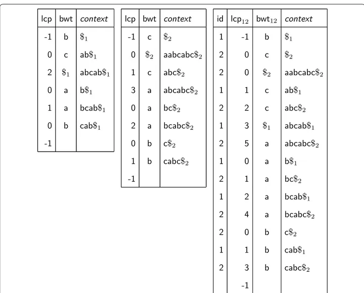
si[1, ni] if j = ni ). Figure 1 shows an example with k = 2 .

(2) bwt1···k[i] =

sj[nj] if sa1···k[i] = �j−1_h=1nh+ 1

sj[sa1···k[i] − �_h=1j−1nh− 1] if �h=1j−1nh+ 1 < sa1···k[i] ≤ �_h=1j nh.

Notice that for k = 1 , this is the usual Burrows–Wheeler Transform [1].

Given the suffix array sa1···k[1, n] of the

concatena-tion s1· · · sk , we consider the corresponding LCP array

lcp_1···k[1, n] defined as in (1) (see again Fig. 1). Note that, for i = 2, . . . , n , lcp1···k[i] gives the length of the longest

common prefix between the contexts of bwt1···k[i] and

bwt1···k[i − 1] . We stress that all practical

implementa-tions use a single $ symbol as end-marker for all strings to avoid alphabet explosion, but end-markers from

Fig. 1 LCP array and BWT for s1= abcab$1 and s2= aabcabc$2 , and multi-string BWT and corresponding LCP array for the same strings. Column

different strings are then sorted as described, i.e., on the basis of the index of the strings they belong to.

Computing multi‑string BWTs

The gSACA-K algorithm [32], based on algorithm SACA-K [33], computes the suffix array for a string collection. Given a collection of strings of total length n, gSACA-K computes the suffix array for their concatenation in O(n)  time using (σ + 1) log n additional bits (in prac-tice, only 2KB are used for ASCII alphabets). gSACA-K is time and space optimal for alphabets of constant size σ =O(1) . The multi-string bwt_1···k of s1, . . . , sk can be

easily obtained from the suffix array as in (2). gSACA-K can also compute the lcp array lcp1···k still in linear time

using only the additional space for the lcp values.

Merging multi‑string BWTs

The Gap algorithm [34], based on an earlier algorithm by Holt and McMillan [35], is a simple procedure for merg-ing multi-strmerg-ing BWTs. In its original formulation the Gap algorithm can also merge LCP arrays, but in this paper we compute LCP values using a different approach more suitable for external memory execution. We describe here only the main idea behind Gap and refer the reader to [34] for further details.

For simplicity in the following we assume we are merging k single-string BWTs bwt1= bwt(s1), . . . , bwtk = bwt(sk) ;

the algorithm does not change in the general case where the inputs are multi-string BWTs. Computing bwt1···k amounts

to sorting the symbols of bwt1, . . . , bwtk according to the

lexicographic order of their contexts, where the context of symbol bwtj[i] is sj[saj[i], nj] . By construction, the symbols

in each bwtj are already sorted by context, hence to

com-pute bwt1···k we only need to merge bwt1, . . . , bwtk without

changing the relative order of the symbols within the input sequences.

The Gap algorithm works in successive iterations. Dur-ing the h-th iteration it computes a vector Z(h)

specify-ing how the entries of bwt1, . . . , bwtk should be merged

to have them sorted according to the first h symbols of their context. Formally, for j = 1, . . . , k the vector Z(h)

contains |bwtj| copies of the value j arranged so that the

following property holds.

Property 1 For j1, j2∈ {1, . . . , k} , the i1-th occurrence of j1 precedes the i2-th occurrence of j2 in Z(h) if and only if the length-h context of bwtj1[i1] is lexicographically

smaller than the length-h context of bwtj2[i2] , or the two

contexts are equal and j1<j2 . 

Property 1 is equivalent to state that we can logically partition Z(h) _{into b(h) + 1 blocks}

such that each block corresponds to the set of symbols in bwt1···k , whose contexts are prefixed by the same

length-h string. The context of any symbol in block Z(h)[ℓj+ 1, ℓj+1] is lexicographically smaller than the

context of the symbols in block Z(h)_[ℓ

k+ 1, ℓk+1] with

k > j ; within each block, if j1<j2 the symbols of bwtj1

precede those of bwtj2 . We keep explicit track of such

blocks using a bit array B[1, n + 1] such that at the end of iteration h it is B[i] �= 0 if and only if a block of Z(h)

starts at position i. By Property 1, when all entries in B are nonzero, Z(h) _{describes how the bwt}

j ( j = 1, . . . , k )

should be merged to get bwt1···k.

Related approaches

The strategy used by Gap to build multi-string BWTs follows the idea, introduced by [35, 36], of merging par-tial BWTs, i.e. BWTs of subsets of the input collection. Interestingly, both previous algorithms for computing the BWT and LCP in external memory [19, 20] are also based on a merging strategy but instead of merging par-tial BWTs, they merge the arrays L1 , L2 , L3 , …, where Li

consists of the symbols which are at distance i from the end of their respective strings. The symbols inside each Li are sorted as usual by context. In the example of Fig. 1,

we would have L1= bc (since s1 ends with b$1 and s2

ends with c$2 ), L2= ab , (since s1 ends with ab$1 and s2

ends with bc$2 ), L3= ca and so on. Note that in L3 c

pre-cedes a since c ’s context ab$1 is lexicographically smaller

than a ’s context bc$2 . Clearly, merging the arrays Li yields

the desired multi-string BWT and the authors of [19, 20] show how to compute also the LCP array. The algorithms in [19, 20] differ in how the merging is done: [19] uses a refinement of a technique introduced in [9, 10], while [20] uses a refinement of Holt and McMillan merging strategy [35, 36].

The _{eGap algorithm}

The eGap algorithm for computing the multi-string BWT and LCP array in external memory works in three phases. First it builds multi-string BWTs for sub-collec-tions in internal memory, then it merges these BWTs in external memory and generates the LCP values. Finally, it sorts the LCP values in external memory.

Phase 1: BWT computation

Given a collection of sequences s1, s2, . . . , sk , we split it

into sub-collections sufficiently small that we can com-pute the multi-string SA for each one of them in internal memory using the gSACA-K algorithm. After computing (3) Z(h)[1, ℓ1], Z(h)[ℓ1+ 1, ℓ2], . . . , Z(h)[ℓb(h)+ 1, n]

each SA, we compute the corresponding multi-string BWT and write it to disk in uncompressed form using one byte per character.

Phase 2: BWT merging and LCP computation

This part is based on the Gap algorithm previously described but suitably modified to work efficiently in external memory (or in semi-external memory if there are at least n bytes of RAM). In the following we assume that the input consists of k BWTs bwt1, . . . , bwtk of total

length n over an alphabet of size σ . The input BWTs are read from disk and never moved to internal memory.

The algorithm initially sets Z(0)_{= 1}n12n2_{. . . k}nk and

B = 10n−11 . Since the context of every symbol is prefixed

by the same length-0 string (the empty string), initially there is a single block containing all symbols. At itera-tion h the algorithm computes Z(h) _{from Z}(h−1) _{as follows}

(see also Fig. 2). We define an array F[1, σ] such that F[c] contains the number of occurrences of characters smaller than c in bwt1···k . F partitions Z(h) into σ buckets, one for

each symbol. Using Z(h−1) _{we scan the partially merged}

BWT, and whenever we encounter the BWT character c coming from bwtℓ , with ℓ ∈ {1, . . . , k} , we store it in the

next free position of bucket c in Z(h) _{; note that c is not}

actually moved, instead we write ℓ in its corresponding position in Z(h) _{. In our implementation, instead of using}

distinct arrays Z(0)_{, Z}(1)_{, . . . we only use two arrays Z}old

and Znew _{, that are kept on disk. At the beginning of}

itera-tion h it is Zold_{= Z}(h−1) _{and Z}new_{= Z}(h−2) _{; at the end}

Znew = Z(h) and the roles of the two files are swapped. While Zold _{is accessed sequentially, Z}new _{is updated}

sequentially within each bucket, that is within each set of positions corresponding to a given character. Since the

boundary of each bucket is known in advance we logi-cally split the Znew _{file in buckets and write to each one}

sequentially.

eGap computes LCP values exploiting the bitvector B used by Gap to mark the beginning of blocks (see Eq. 3) within each Z(h) _{(for simplicity the computation of B is}

not shown in Fig. 2). We observe that if B[i] is set to 1 during iteration h then lcp1···k[i] = h − 1 , since the

algo-rithm has determined that the contexts of bwt1···k[i] and

bwt1···k[i − 1] have a common prefix of length exactly

h −1 . We introduce an additional bit array Bx[1, n + 1]

such that, at the beginning of iteration h, Bx[i] = 1 iff B[i] has been set to 1 at iteration h − 2 or earlier. During iteration h, if B[i] = 1 we look at Bx[i] . If Bx[i] = 0 then

we know that B[i] has been set at iteration h − 1 : thus we output to a temporary file Fh−2 the pair �i, h − 2� to

record that lcp1···k[i] = h − 2 , and we set Bx[i] = 1 so no

pair for position i will be produced in the following itera-tions. At the end of iteration h, file Fh−2 contains all pairs

�i, lcp_1···k[i]� with lcp[i] = h − 2 ; the pairs are written in increasing order of their first component, since B and Bx

are scanned sequentially. These temporary files will be merged in Phase 3 to produce the LCP array.

As proven in [34, Lemma  7], if at iteration h of the Gap algorithm we set B[i] = 1 , then at any iteration g ≥ h +2 processing the entry Z(g)[i] will not change the arrays Z(g+1) _{and B. Since the roles of the Z}old _and

Znew files are swapped at each iteration, and at iteration h we scan Zold_{= Z}(h−1) _{to update Z}new _{from Z}(h−2) _to

Z(h) , we can compute only the entries Z(h)[j] that are dif-ferent from Z(h−2)_{[j] . In particular, any range [ℓ, m] such}

that Bx[ℓ] = Bx[ℓ + 1] = · · · = Bx[m] = 1 can be added

to a set of irrelevant ranges that the algorithm may skip

Fig. 2 Outline of Gap’s main loop computing Z(h) _{from Z}(h−1) _{. Array F is initialized so that F[c] contains the number of occurrences of symbols}

in successive iterations (irrelevant ranges are defined in terms of the array Bx as opposed to the array B, since

before skipping an irrelevant range we need to update both Zold _{and Z}new _{). We read from one file the ranges to}

be skipped at the current iteration and simultaneously write to another file the ranges to be skipped at the next iteration (note that irrelevant ranges are created and con-sumed sequentially). Since skipping a single irrelevant range takes O(k + σ) time, an irrelevant range is stored only if its size is larger than a given threshold t and we merge consecutive irrelevant ranges whenever possible. In our experiments we used t = max(256, k + σ) . In the worst case the space for storing irrelevant ranges could be O(n) but in actual experiments it was always less than 0.1n bytes.

As in the Gap algorithm, when all entries in B are nonzero, Zold _{describes how the BWTs bwt}

j ( j = 1, . . . , k )

should be merged to get bwt1···k , and a final sequential

scan of the input BWTs along with Zold _{allows to write}

bwt1···k to disk, in sequential order. Our implementation

can merge at most 27_{= 128 BWTs at a time because we}

use 7 bits to store each entry of Zold _{and Z}new _{. These}

arrays are maintained on disk in two separate files; the additional bit of each byte are used to keep the current and the next copy of B. The bit array Bx is stored

sepa-rately in a file of size n/8 bytes. To merge a set of k > 128 we split the input in subsets of cardinality 128 and merge them in successive rounds. In practice, the algorithm merges the multi-string BWTs produced by Phase 1. In our experiments the maximum number of sub-collec-tions was 21.

Semi-external version We have also implemented a semi-external version of the merge algorithm that uses n bytes of RAM. The i-th byte is used to store Zold_{[i] and}

Znew[i] (3 bits each), B[i] and Bx[i] . This version can sort

at most 23_{= 8 BWTs simultaneously; to sort k BWTs it}

performs log8k merging rounds. Although performing

more rounds is clearly more expensive, this version stores in RAM all the arrays that are modified and reads from disk only the input BWTs and is therefore significantly faster.

Phase 3: LCP merging

At the end of Phase 2 all LCP-values have been written to the temporary files Fh on disk as pairs �i, lcp[i]� . Each file

Fh contains all pairs with second component equal to h

in order of increasing first component. The computation of the LCP array is completed using a standard external memory multiway merge [37, Chap.  5.4.1] of maxlcp sorted files, where maxlcp = maxi(lcp1···k[i]) is the

larg-est LCP value.

Analysis

During Phase 1, gSACA-K computes the suffix array for a sub-collection of total length m using 9m bytes (8m bytes for sa and 1m bytes for the text). If the available RAM is M, the input is split into subcollections of size ≈ M/9 . Since gSACA-K runs in linear time, if the input collec-tion has total size n, Phase 1 takes O(n) time overall.

A single iteration of Phase 2 consists of a complete scan of Z(h−1) _{except for the irrelevant ranges. Since the}

algo-rithm requires maxlcp iterations, without skipping the irrelevant ranges the algorithm would require maxlcp sequential scans of O(n) items. Reasoning as in [34, Theorem 8] we get that by skipping irrelevant ranges the overall amount of data directly read/written by the algo-rithm is O(n avelcp) items where avelcp is the aalgo-rithmetic average of the entries in the final LCP array. However, if we reason in terms of disk blocks, every time we skip an irrelevant range we discard the current block and load a new one (unless the beginning of the new relevant range is inside the same block; in that case or if the beginning of the new relevant range is in the block immediately fol-lowing the current one, skipping the irrelevant range does not save any I/O). We can upper bound this extra cost, with an overhead of O(1) blocks for each irrelevant range skipped. Summing up, if the total number of skipped ranges is Ir and each disk block consists of B words, the I/O complexity of Phase 2 according to the theoretical model in [15] is O(Ir + n avelcp/(B log n)) block I/Os (under the reasonable assumptions that the alphabet is constant, each entry in Z takes constant space, and we need a constant number of merge rounds). Although the experiments in “Experiments” section suggest that in practice Ir is small, for simplicity and uniformity with the previous literature we upper bound the cost of Phase 2 with O(n maxlcp) sequential I/Os (corresponding to O(n maxlcp/(Blog n)) block I/Os).

Phase 3 takes O(⌈logmaxlcp⌉) rounds; each round

merges  LCP files by sequentially reading and writing O(n) bytes of data. The overall cost of Phase 3 is therefore O(nlogmaxlcp) sequential I/Os. In our experiments we

used  = 256 ; since in our tests maxlcp < 216 _two

merg-ing rounds were always sufficient. Experiments

In this section we report on an experimental study comparing between the eGap algorithm and the other known external memory tools computing the BWT and LCP arrays of sequence collections. We imple-mented eGap in ANSI C based on the code of Gap [34] and gSACA-K [32]. eGap source code is freely available at https ://githu b.com/felip elouz a/egap/. All tested algorithms were compiled with GNU GCC ver.

4.6.3, with optimizing option -O3. The experi-ments were conducted on a machine with GNU/Linux Debian 7.0/64 bits operating system using an Intel i7-3770 3.4 GHz processor with 8 MB cache, 32 GB of RAM and a 2.0 TB SATA hard disk with 7200 RPM and 64 MB cache. The complete set of experi-ments took about 70 days of computing time.

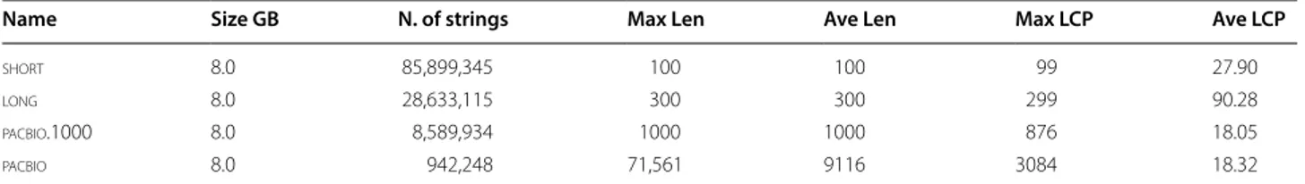
Datasets We used four real DNA datasets reported in Table 1 containing sequences of different lengths and structure. The sequences of the first three datasets were trimmed to make them of the same length, while the fourth dataset contains sequences of widely different lengths. short are Illumina reads from human genome (ftp://ftp.sra.ebi.ac.uk/vol1/ERA01 5/ERA01 5743/srf/). long are Illumina HiSeq 4000 paired-end RNA-seq reads from plant Setaria viridis (https ://trace .ncbi.nlm. nih.gov/Trace s/sra/?run=ERR19 42989 ). pacbio.1000 and pacbio are PacBio RS II reads from Triticum aes-tivum (wheat) genome (https ://trace .ncbi.nlm.nih.gov/ Trace s/sra/?run=SRR58 16161 ). All datasets contain sequences over the A, C, G, T alphabet plus a string terminator symbol.

Memory setting To make a realistic external memory experimental setting one has to use an amount of RAM smaller than the size of the data. Indeed, if more RAM is available, even if the algorithm is supposedly not using it, the operating system will use it to temporar-ily store disk data and the algorithm will be no longer really working in external memory. This phenomenon will be apparent also from our experiments. For these reasons we reduced the available RAM to simulate three different scenarios: (i) input data 4 times larger than the available RAM, (ii) input data of approximately the same size as the RAM, and (iii) input data 4 times smaller than the RAM. We evaluated these scenarios with the complete 8  GB datasets from Table 1 (with 2  GB, 8  GB, and 32  GB RAM), and with the datasets trimmed to 1 GB (hence with 256 MB, 1 GB, and 4 GB RAM). The RAM was limited at boot time to a value equal to the amount assigned to the algorithm plus a small extra amount for the operating system (14 MB for the 256 MB instance and 64 MB for the others).

Comparison with the existing algorithms

We compared eGap with the algorithm BCR [19] which is the current state of the art for BWT/LCP computation for collections of sequences. We used the bcr-lcp implementation from [38] since the previous implementation mentioned in [19] did not compute the LCP values correctly. We tested also the recently proposed algorithm bwt-lcp-em [20] using the code from [39]. As a reference we also tested the algorithm eGSA [14] using the code from [40]. eGSA computes the Suffix and LCP Arrays for collections of sequences in external memory: the disadvantage of this algorithm is that working with the Suffix Array could involve transferring to/from disk a much larger amount of data.

Limitations We tested bwt-lcp-em only on the short 1 GB dataset since the implementation in [39] only supports collections of at most 2 GB and with strings of at most 253 symbols. We tested eGSA only with memory scenario (iii) (input data 4 times smaller than the RAM) since it was already observed in [14] that eGSA ’s running time degrades when the RAM is restricted to the input size. Finally, we could not test bcr-lcp on the pacbio 1 GB dataset since it stopped with an internal error after four days of computation. This is probably due to the presence of very long strings in the dataset since bcr-lcp was originally conceived for collections of short/medium length strings. The corresponding entries are marked as “failed” in Fig. 3. For the larger 8 GB data-sets we stopped the experiments that did not complete after six days of CPU time, corresponding to 60 micro-seconds per input symbol. The corresponding entries are marked with “ > 60 ” in Fig. 3. Note that both bwt-lcp-em and bcr-lcp are active projects, so some of the lim-itations reported here could have been solved after our experiments were completed.

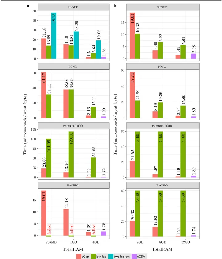
Results: The results of our experiments are summarized in Fig. 3. The bar plots on the left are for the 1 GB data-sets showing the running time as function of the available RAM; the diagrams on the right are for the 8 GB data-sets. The results show that for memory scenarios (i) and (ii) eGap and bcr-lcp have the better performance, whereas for scenario (iii) eGap and eGSA are the best

Table 1 Datasets used in our experiments

Columns 4 and 5 show the maximum and average lengths of the single strings. Columns 6 and 7 show the maximum and average LCPs of the collections

Name Size GB N. of strings Max Len Ave Len Max LCP Ave LCP

short 8.0 85,899,345 100 100 99 27.90

long 8.0 28,633,115 300 300 299 90.28

pacbio.1000 8.0 8,589,934 1000 1000 876 18.05

options. The performance of bwt-lcp-em improves with the RAM size, but it is still 12 times slower than eGap for the short datasets with 4 GB of RAM.

The above results are in good accordance with the the-oretical analysis. bcr-lcp complexity is O(n maxlen) sequential I/Os while eGap and bwt-lcp-em both take

a b 48.18 13.69 21.18 28.29 13.89 14.9 1.75 19.06 5.64 1.5 31.11 61.17 38.09 38.06 1.99 15.11 3.16 101.09 23.68 120.15 13.26 1.7 2 51.68 1.2 9 failed 19.01 failed 11.18 1.7 5 failed 1.3 9 pacbio pacbio.1000 long short 256MB 1GB 4GB 0 10 20 30 40 50 0 20 40 60 0 25 50 75 100 125 0 5 10 15 TotalRAM Time (microseconds/input byte) 10.33 19.03 6.82 3.46 2.08 5.61 1.49 21.99 57.71 19.36 8.18 1.89 15.69 2.74 > 60 21.52 > 60 3.9 7 1.8 9 > 60 1.1 9 > 60 20.63 > 60 12.92 1.7 4 > 60 1.2 3 pacbio pacbio.1000 long short 2GB 8GB 32GB 0 5 10 15 0 20 40 60 0 20 40 60 0 20 40 60 TotalRAM Time (microseconds/input byte)

eGap bcr-lcp bwt-lcp-em eGSA

O(n maxlcp) sequential I/Os. For the short and long datasets the maximum length and the maximum LCP coincide and we see that when the available memory is only one fourth of the input size bcr-lcp is clearly the fastest option: indeed it is up to a factor 2.6 faster than eGap. This is no longer true when the available memory is equal or larger than the input size: in this case eGap is the fastest, probably because of its ability to exploit all the available memory using a semi-external strategy when-ever possible. When the available memory is larger than the input size or for the pacbio.1000 dataset which has a very large maxlen then eGap is up to 40 times faster than bcr-lcp. Note that, in accordance with our heuristic analysis, eGap ’s running time per input byte appears to be roughly proportional to the average LCP of the collec-tion. If we look at the datasets pacbio and pacbio.1000 we see that they have widely different maximum LCPs, yet their running times are very close similarly to their average LCPs.

Note that in the scenario (iii) eGSA is often the fast-est algorithm and its running time appears to be less influenced by the size of the average or maximum LCP. Another advantage is that it also computes the Suffix Array, but it has the drawback of using a large amount of disk working space: 340 GB for a 8 GB input vs 56 GB used by eGap.

We conclude that, although eGap is not always the fastest algorithm, its running time is never too far from that of the best algorithm. In addition, eGap is the only algorithm that was able to complete all computations in all memory models. Although it was devised as an exter-nal memory algorithm, its ability to switch to a semi-external strategy if the memory is available makes it a very flexible tool. The comparison with the other algo-rithms in this setting is indeed not completely fair, since none of them is designed to take the available memory as a parameter in order to make the best use of it. Note that, as the available memory increases, all algorithms become faster because the operating system uses the RAM as a buffer but the speed improvement is different for differ-ent algorithms.

Relative performance of _{eGap’s building blocks}

We evaluated the percentage of time spent by each phase of eGap and their efficiency (percentage the CPU was busy) on the 8 GB datasets in the memory scenarios con-sidered above, thus with RAM limited to (i) 1  GB, (ii) 8 GB, and (iii) 32 GB.

The results in Fig. 4 show that Phase 2 of eGap domi-nates the algorithm in general. The second phase took about 95% , 85% and 50% of the total time in scenarios (i), (ii), and (iii) respectively. If we look at the efficiency of the single phases, we see that they all improve with the RAM

size. However, we notice that for any given memory sce-nario the efficiency of Phases 1 and 3 was almost the same for the different datasets, while Phase 2 has a dif-ferent behavior. For the short and long datasets with 8 GB and 32 GB RAM, we see that Phase 2 efficiency is very close to Phase 1’s, while there is a sharp drop when using 2 GB RAM. For the pacbio datasets, the drop in Phase 2 efficiency is significant already when we use 8 GB RAM.

Applications

In this section we show that the eGap algorithm, in addi-tion to the BWT and LCP arrays, can output addiaddi-tional information useful to design efficient external memory algorithms for three well known problems on sequence collections: (i) the computation of maximal repeats, (ii) the all pairs suffix–prefix overlaps, and (iii) the construc-tion of succinct de Bruijn graphs. For these problems we describe algorithms which are derived from known (internal memory) algorithms suitably modified so that they process the input data in a single sequential scan.

Our first observation is that eGap can also output the array which provides, for each bwt entry, the id of the sequence to which that entry belongs. In information retrieval this is usually called the Document Array, so in the following we will denote it by da . In Phase 1 the gSACA-K algorithm can compute the da together with the lcp and bwt using only additional 4n bytes of space to store the da entries. These partial da ’s can be merged in Phase 2 using the Znew _{array in the same way as the}

BWT entries. In the following we use bwt , lcp , and da to denote the multistring BWT, LCP and Document Array of a collection of m sequences of total length n. We write s to denote the concatenation s1· · · sm and sa to denote

the suffix array of s . We will use s and sa to describe and prove the correctness of our algorithms, but neither s nor sa are used in the computations.

Computation of maximal repeats

Different notions of maximal repeats have been used in the bioinformatics literature to model different notions of repetitive structure (see for example [21, 22]). We use a notion of maximal repeat from [41, Chap. 7]: we say that a string α is a Type 1 maximal repeat if α occurs in the collection at least twice and every extension, i.e. cα or αc with c ∈  , occurs fewer times. We consider also a more restrictive notion: we say that a string α is a Type 2 maxi-mal repeat if α occurs in the collection at least twice and every extension of α occurs at most once.

To compute Type 1 maximal repeats the crucial obser-vation is that there is a substring of length ℓ that prefixes sa entries j, j + 1, . . . , i (and no others) iff lcp[k] ≥ ℓ for k = j +1, . . . , i , and both lcp[j] and lcp[i + 1] are smaller

than ℓ . To ensure that the repeat is Type 1 maximal, we also require that there exists h ∈ [j + 1, i] such that lcp[h] = ℓ and that the substring bwt[j, i] contains at least two distinct characters.

Our algorithm consists of a single sequential scan of bwt and lcp . During the scan, we maintain a stack containing pairs �j, lcp[h]� with j ≤ h such that if �j′_{, lcp[h}′_{]� is below �j, lcp[h]� then j}′_{<j and}

a b pacbio pacbio.1000 long short 2GB 8GB 32GB 0.00 0.25 0.50 0.75 1.00 0.00 0.25 0.50 0.75 1.00 0.00 0.25 0.50 0.75 1.00 0.00 0.25 0.50 0.75 1.00 TotalRAM Pe rcentageoftherunningtime pacbio pacbio.1000 long short 2GB 8GB 32GB 0.00 0.25 0.50 0.75 1.00 0.00 0.25 0.50 0.75 1.00 0.00 0.25 0.50 0.75 1.00 0.00 0.25 0.50 0.75 1.00 TotalRAM Efficiency (CPU/totaltime)

Phase 1 Phase 2 Phase 3

lcp[h′_{] < lcp[h] . In addition, when the scanning reaches}

position i, for every entry �j, lcp[h]� in the stack it is lcp[h] = min_j≤k<ilcp[k] , that is, lcp[h] is the smallest value in the range lcp[j, i − 1].

We maintain the stack as follows. When we reach position i, if the entry �j, lcp[h]� at the top of the stack has lcp[h] < lcp[i] we push �i, lcp[i]� on the stack. If lcp[h] = lcp[i] we do nothing. If lcp[h] > lcp[i] we pop from the stack all entries �j, lcp[h]� with lcp[h] > lcp[i] ; if the removal leaves at the top of the stack an entry �j′_{, lcp[h}′_{]� with lcp[h}′_{] < lcp[i] we push on the stack a}

new entry � ˆ, lcp[i]� where ˆ is the first component of the last entry just removed from the stack. Note that in any case when we have completed the processing of position i the entry at the top of the stack has sec-ond component equal to lcp[i] , and for each stack entry �j, lcp[h]� it is lcp[h] = min_j≤k≤ilcp[k] as claimed.

We now prove that if �j′_{, lcp[h}′_{]� is immediately below}

�j, lcp[h]� then lcp[j − 1] = lcp[h′_{]. As we observed}

above, if at step i we push �i, lcp[i]� on the stack, the previous top entry has second component equal to lcp[i − 1] so the property holds for the first insertion of an entry �i, lcp[·]� . During the following steps it is pos-sible that �i, lcp[x]� is removed and immediately rein-serted as �i, lcp[y]� (with lcp[y] < lcp[x] ), but since the preceding stack element does not change, is still holds true that lcp[i − 1] is equal to the second component of the preceding element. Note that, since lcp values on the stack are strictly increasing, we conclude that for each stack entry �j, lcp[h]� it is lcp[j − 1] < lcp[h].

Our algorithm outputs Type 1 maximal repeats when elements are popped from the stack. At step i +1 we pop from the stack all entries �j, lcp[h]� such that lcp[h] > lcp[i + 1] . Recall that by construction lcp[h] = min_j≤k≤ilcp[k] . In addition lcp[j − 1] < lcp[h] and lcp[i + 1] < lcp[h] . Thus, to ensure that we have found a Type 1 maximal repeat we only need to check that bwt[j − 1, i] contains at least two distinct charac-ters. To efficiently check this latter condition, for each stack entry �j, lcp[h]� we maintain a bit vector bj of size

σ keeping track of the distinct characters in the array bwt from position j − 1 to the next stack entry, or to the last seen position for the entry at the top of the stack. When �j, lcp[h]� is popped from the stack its bit vector is or-ed to the previous stack entry in constant time; if �j, lcp[h]� is popped from the stack and immediately replaced with �j, lcp[i]� its bit vector survives as it is (essentially because it is associated with an index, not with a stack entry). Clearly, maintaining the bit vector does not increase the asymptotic cost of the algorithm.

Since at each step we insert at most one entry on the stack, the overall cost of our algorithm is O(n) time. The algorithm uses a stack of size bounded by O(maxlcp)

words. For most applications maxlcp ≪ n so it should be feasible to keep the stack in RAM. However, since a stack can also be implemented in external memory in O(1) amortized time per operation [42], we can state the fol-lowing result.

Theorem  1 We can compute all Type 1 maximal repeats in O(n) time executing a single scan of the arrays bwt and lcp using O(1) words of RAM. 

To find Type 2 maximal repeats, we are interested in consecutive LCP entries lcp[j], lcp[j + 1], . . . , lcp[i], lcp[i + 1], such that lcp[j] < lcp[j + 1] = lcp[j + 2] = · · · =lcp[i] > lcp[i + 1]. Indeed, this implies that for h = j, . . . , i all suffixes s[sa[h], n] are prefixed by the same string α of length lcp[j + 1] and every extension αc occurs at most once. If this is the case, then α is a Type 2 maxi-mal repeat if all characters in bwt[j, i] are distinct since this ensures that also every extension cα occurs at most once. In order to detect this situation, as we scan the lcp array we maintain a candidate pair �j + 1, lcp[j + 1]� such that j + 1 is the largest index seen so far for which lcp[j] < lcp[j + 1] . When we establish a candidate at

j +1 as above, we initialize to zero a bit vector b of size σ setting to 1 only entries bwt[j] and bwt[j + 1] . As long as the following values lcp[j + 2], lcp[j + 3], . . . are equal to lcp[j + 1] we go on updating b and if the same posi-tion is marked twice we discard �j + 1, lcp[j + 1]� . If we reach an index i + 1 such that lcp[i + 1] > lcp[j + 1] , we update the candidate to �i + 1, lcp[i + 1]� and reinitialize b. If we reach i + 1 such that lcp[i + 1] < lcp[j + 1] and �j + 1, lcp[j + 1]� has not been discarded, then a repeat of

Type 2 (with i − j + 1 repetitions) has been located.

Theorem  2 We can compute all Type 2 maximal repeats in O(n) time executing a single scan of the arrays bwt and lcp using O(1) words of RAM. 

Note that when our algorithms discover Type 1 or Type 2 maximal repeats we know the repeat length and the number of occurrences so one can easily filter out non-interesting repeats (too short or too frequent). In some applications, for example the MUMmer tool [43], one is interested in repeats that occur in at least r distinct input sequences, maybe exactly once for each sequence. Since for these applications the number of input sequences is relatively small, we can handle these requirements by simply scanning the da array simultaneously with the lcp and bwt arrays and keeping track of the sequences associ-ated to a maximal repeat using a bit vector (or a union-find structure) as we do with characters in the bwt.

All pairs suffix–prefix overlaps

In this problem we want to compute, for each pair of sequences si sj , the longest overlap between a suffix of si

and a prefix of sj . Our solution is inspired by the

algo-rithm in [24] which in turn was derived by an earlier Suf-fix-tree based algorithm [23]. The algorithm in [24] solves the problem using a Generalized Enhanced Suffix array (consisting of the arrays sa , lcp , and da ) in O(n + m2₎

time, which is optimal since n is the size of the input and there are m2 _{longest overlaps. However, for large}

col-lections it is natural to consider the problem of report-ing only the overlaps larger than a given threshold τ still spending O(n) time plus constant time per reported over-lap. Our algorithm solves this more challenging problem.

In the following we say that a suffix starting at sa[i] is special iff it is a prefix of the suffix starting at sa[i + 1] , not considering the end-marker. This is equivalent to state that s[sa[i] + lcp[i + 1]] = $ . For example, in Fig. 1 (right) the special suffixes are ab$1 , abc$2 , abcab$1

b$1 , bc$2 , bcab$1 , c$2 , cab$1 . Notice that a special

suf-fix starting at sa[i] has the form v$ with |v| = lcp[i + 1] ; clearly only if sa[i] is special then v can be a suffix–pre-fix overlap. Note also that any sufsuffix–pre-fix $ is always trivially special.

To efficiently solve the suffix–prefix overlaps problem, we modify Phase  2 of our algorithm so that it outputs also the bit array xlcp such that xlcp[i] = 1 iff the suf-fix starting at sa[i] is special. To this end, we maintain an additional length-n bit array S such that, at the end of iteration h, S[i] = 1 if and only if the suffix starting at sa[i] is special and it has length less than h, again not considering the end-marker symbol. The array S is initial-ized at the end of iteration h = 1 as S = 1k₀n−k _,

consist-ently with the fact that in the final suffix array the first k contexts are strings consisting of just an end-marker, that are special suffixes and the only suffixes of length 0.

During iteration h, we update S as follows. With ref-erence to the code in Fig. 2, whenever we use entry Z(h−1)[i] to compute Z(h)_{[j] for some j, if S[i] = 1 and}

B[j +1] = 0 then we set S[j] = 1.

Lemma 1 The above procedure correctly updates the array S.

Proof We prove by induction that at the end of itera-tion h: (1) S[i] = 1 iff the suffix starting at sa[i] is special and has length less than h, and (2) if S[i] = 1 the length-h context currently in position i is in tlength-he correct lexico-graphic position with respect to the final suffix array ordering (in other words, it is a prefix for s[sa[i], n]). For h = 1 the result is true by construction. During itera-tion h > 1 , if we reach a posiitera-tion i such that S[i] = 1 , then by inductive hypothesis the context in position i has

the form v$ with |v| ≤ h − 2 . If c is the symbol we read at Step 5 of Fig. 2, then the context corresponding to posi-tion j is cv$ . Since the context contains the end-marker, j is the correct lexicographic position of cv$ which is there-fore the suffix corresponding to sa[j] . If B[j + 1] = 0 , then lcp[j + 1] ≥ h − 1 . Since lcp[j + 1] ≤ |cv| ≤ h − 1 , it follows that |cv| = lcp[j + 1] = h − 1 and S[j] is special as claimed.

On the other hand, if at the end of iteration h it is S[j] = 0 , then either it was S[i] = 0 or B[j + 1] = 1 which implies lcp[j + 1] < h − 1 . In both cases the suffix start-ing at sa[j] cannot be special and of length less than h. 

Having established the properties of S, we can now show how to compute xlcp . Recall that LCP values are computed as follows. In Phase 2, during iteration h + 1 if B[i + 1] = 1 and Bx[i + 1] = 0 we output the pair

�i + 1, h − 1� recording the fact that lcp[i + 1] = h − 1 . Such pairs are later sorted by their first component dur-ing Phase 3 to retrieve the LCP array. If sa[i] is special, its corresponding suffix has length lcp[i + 1] = h − 1 so, by the properties of S, at the beginning of itera-tion h + 1 it is S[i] = 1 . Thus, to compute xlcp , instead of the pair �i + 1, h − 1� we output the triplet �i + 1, h − 1, S[i]� = �i + 1, lcp[i + 1], xlcp[i]� . After the

merging is completed we sort the triplets by their first component and we derive both arrays lcp and xlcp.

Our algorithm for computing the suffix–prefix over-laps longer than a threshold τ , consists of a sequential scan of the arrays bwt , lcp , da , and xlcp . We maintain m distinct stacks, stack[1], . . . , stack[m] , one for each input sequence; stack[k] stores pairs �j, lcp[j + 1]� only if sa[j] is a special suffix belonging to sequence k such that lcp[j + 1] > τ . During the scan we maintain the invariant that for all stack entries �j, lcp[j + 1]� , lcp[j + 1] is the length of the longest common prefix (longer than τ ) between s[sa[j], n] and s[sa[i], n] , where i is the posi-tion just scanned.

To maintain the invariant in amortized constant time per scanned position, we use the following additional structures:

• A stack lcpStack containing, in increasing order, the values ℓ such that some stack[k] contains an entry with LCP component equal to ℓ;

• An array of lists top such that top[ℓ] contains the indexes k for which the entry at the top of stack[k] has LCP component equal to ℓ;

• An array daPtr[1, m] such that daPtr[k] points to the entry k in the list top[ℓk] containing it ( daPtr[k] is

used to remove such entry k from top[ℓk] in constant

We maintain the above data structures as follows. When we reach position i + 1 we remove all entries �j, lcp[j + 1]� such that lcp[j + 1] > lcp[i + 1] . We use lcpStack to determine which are the values ℓ such that some stack contains an entry j, ℓ with ℓ > lcp[i + 1] . For the value ℓ at the top of lcpStack we locate through top[ℓ] all stacks that contain an ℓ-entry at the top. For each one of these stacks we remove the top entry j, ℓ so that a new entry �j′_{, ℓ}′_{� , with ℓ}′_{< ℓ , becomes the new top of}

the stack. Then, if k is the stack that is being updated, we add k to top[ℓ′_{] , and a pointer to the new entry is saved}

in daPtr[k] (overwriting the previous pointer). When all entries of top[ℓ] have been processed, top[ℓ] is emptied and ℓ is popped from lcpStack . The whole procedure is repeated until a value ℓ ≤ lcp[i + 1] is left at the top of lcpStack.

Finally, if xlcp[i] = 1 and lcp[i + 1] > τ , �i, lcp[i + 1]� is added to stack[da[i]] ; this requires removing da[i] from the list top[ℓ] where ℓ is the previous top LCP value in stack[da[i]] ; the position of da[i] in top[ℓ] is retrieved through daPtr[da[i]] . Also we add da[i] to top[lcp[i + 1]] , and the pointer to this new element of top[lcp[i + 1]] is written to daPtr[da[i]] . Since the algorithm performs an amortized constant number of operations per entry �i, lcp[i + 1]� , maintaining the above data structures takes O(n) time overall.

The computation of the overlaps is done as in [24]. When the scan reaches position  i, we check whether bwt[i] = $ . If this is the case, then s[sa[i], n] is prefixed by the whole sequence sda[i] , hence the longest overlap

between a prefix of sda[i] and a suffix of sk is given by the

element currently at the top of stack[k] , since by con-struction these stacks only contain special suffixes whose overlap with s[sa[i], n] is larger than τ . Note that using lcpStack and top we can directly access the stacks whose top element corresponds to an overlap with sda[i] larger

than τ , hence the time spent in this phase is proportional to the number of reported overlaps. As in [24] some care is required to handle the case in which the whole string sda[i] is a suffix of another sequence, but this can be done

without increasing the overall complexity as in [24]. Since we spend constant time for reported overlap and amor-tized constant time for scanned position the overall cost of the algorithm, in addition to the scanning of the bwt /lcp/xlcp/da arrays, is O(n + Eτ) , where Eτ is the number

of suffix–prefix overlaps greater than τ . Since all stacks can be implemented in external memory spending amor-tized constant time per operation, we only need to store in RAM top and daPtr that overall take O(m + maxlcp) words.

Theorem  3 Our algorithm computes all suffix–prefix overlaps longer than τ in time O(n + Eτ) , where Eτ is the

number of reported overlaps, using O(m + maxlcp) words of RAM and executing a single scan of the arrays bwt , lcp ,

da and xlcp . 

Construction of succinct de Bruijn graphs

A recent remarkable application of compressed data structures is the design of efficiently navigable succinct representations of de Bruijn graphs [26–28]. Formally, a de Bruijn graph for a collection of strings consists of a set of vertices representing the distinct k-mers appearing in the collection, with a directed edge (u, v) iff there exists a (k + 1)-mer α in the collection such that α[1, k] is the k-mer associated to u and α[2, k + 1] is the k-mer associ-ated to v.

The starting point of all de Bruijn graphs succinct rep-resentation is the BOSS reprep-resentation [28], so called from the authors’ initials. For simplicity we now describe the BOSS representation of a k-order de Bruijn graph using the lexicographic order of k-mers, instead of the co-lexicographic order as in [28], which means we are building the graph with the direction of the arcs reversed. This is not a limitation since arcs can be traversed in both directions (or we can apply our construction to the input sequences reversed).

Consider the N k-mers appearing in the collection sorted in lexicographic order. For each k-mer αi

con-sider the array Ci of distinct characters c ∈  ∪ {$} such

that cαi appears in the collection. The concatenation

W = C1C2· · · CN is the first component of the BOSS

representation. The second component is a binary array last , with |last| = |W | , such that last[j] = 1 iff W [j] is the last entry of some array Ci . Clearly, there is a bijection

between entries in W and graph edges; in the array last each sequence 0i_{1 ( i ≥ 0 ) corresponds to the outgoing}

edges of a single vertex with outdegree i + 1 . Finally, the third component is a binary array W− _{, with |W}−_{| = |W | ,}

such that W−_{[j] = 1 iff W [j] comes from the array C} i ,

where αi is the lexicographically smallest k-mer prefixed

by αi[1, k − 1] and preceded by W[j] in the collection.

This means that αi is the lexicographically smallest k-mer

with an outgoing edge reaching the node associated to k-mer W [j]αi[1, k − 1] . Note that the number of 1 ’s in last

and W− _{is exactly N, i.e. the number of nodes in the de}

Bruijn graph.

We now show how to compute W , last and W− _by

a sequential scan of the bwt and lcp array. The crucial observation is that the suffix array range prefixed by the same k-mer αi is identified by a range [bi, ei] of LCP

val-ues satisfying lcp[bi] < k , lcp[ℓ] ≥ k for ℓ = bi+ 1, . . . , ei

and lcp[ei+ 1] < k . Since k-mers are scanned in

lexi-cographic order, by keeping track of the corresponding characters in the array bwt[bi, ei] we can build the array Ci

and consequently W and last . To compute W− _{we simply}

need to keep track also of suffix array ranges correspond-ing to (k − 1)-mers. Every time we set an entry W [j] = c we set W−_{[j] = 1 iff this is the first occurrence of c in the}

range corresponding to the current (k − 1)-mers.

Theorem  4 Our algorithm computes the BOSS repre-sentation of a de Bruijn graph in O(n) time using O(1) words of RAM, and executing a single scan of the arrays

bwt and lcp . 

If, in addition to the bwt and lcp arrays, we also scan the da array, then we can keep track of which sequences contain any given graph edge and therefore obtain a suc-cinct representation of the colored de Bruijn graph [44]. Finally, we observe that if our only objective is to build the k-order de Bruijn graph, then we can stop the phase 2 of our algorithm after the k-th iteration. Indeed, we do not need to compute the exact values of LCP entries greater than k, and also we do not need the exact BWT but only the BWT characters sorted by their length  k context.

Conclusions

In this paper we have described eGap, a new algorithm for the computation of the BWT and LCP arrays of large collection of sequences. Depending on the amount of available memory, eGap uses an external or semi-exter-nal strategy for computing the BWT and LCP values. An experimental comparison of the available tools for BWT and LCP arrays computation shows that eGap is the fast-est tool in many scenarios and was the only tool capable of completing the computation within a reasonable time frame for all kind of input data.

Another important feature of eGap is that, in addition to the BWT and LCP array, it can compute, without any asymptotic slowdown, two additional arrays that pro-vide important information about the substrings of the input collection. We show how to use such information to design efficient external memory algorithms for three important problems for biosequences, namely the com-putation of maximal repeats, the comcom-putation of the all pairs suffix–prefix overlaps, and the construction of suc-cinct de Bruijn graphs. Overall our results confirm the importance of the BWT and LCP arrays beyond their use for the construction of compressed full text indexes. This is in accordance with other recent results that have shown of they can be used directly to discover structural information on the underlying collection (see [45–47] and references therein).

Authors’ contributions

LE and GM devised the main algorithmic ideas. All authors contributed to improve the algorithms and participated to their implementations. FAL and

GPT designed and performed the experiments. All authors read and approved the final manuscript.

Author details

1 _{DiSIT, University of Eastern Piedmont, Viale Michel, 11, 15121 Alessandria,} Italy. 2 _{Department of Computing and Mathematics, University of São Paulo,} Av. Bandeirantes, 3900, 14040-901 Ribeirão Preto, Brazil. 3 _{IIT CNR, Via Moruzzi,} 1, 56124 Pisa, Italy. 4 _{Institute of Computing, University of Campinas, Av. Albert} Einstein, 1251, 13083-852 Campinas, Brazil.

Competing interests

The authors declare that they have no competing interests.

Availability

The source code of the proposed algorithm is available at https ://githu b.com/

felip elouz a/egap.

Funding

L.E. was partially supported by the University of Eastern Piedmont project Behavioural Types for Dependability Analysis with Bayesian Networks. F.A.L. was supported by the Grants #2017/09105-0 and #2018/21509-2 from the São Paulo Research Foundation (FAPESP). G.M. was partially supported by PRIN grant 201534HNXC and INdAM-GNCS Project 2019 Innovative methods for the solution of medical and biological big data. G.P.T. acknowledges the support of Brazilian agencies Conselho Nacional de Desenvolvimento Científico e Tecnológico (CNPq) and Coordenação de Aperfeiçoamento de Pessoal de Nível Superior (CAPES).

Publisher’s Note

Springer Nature remains neutral with regard to jurisdictional claims in pub-lished maps and institutional affiliations.

Received: 6 November 2018 Accepted: 23 February 2019

References

1. Burrows M, Wheeler DJ. A block-sorting lossless data compression algo-rithm. Technical report, Digital SRC Research Report; 1994.

2. Mäkinen V, Belazzougui D, Cunial F, Tomescu AI. Genome-Scale Algorithm Design: biological sequence analysis in the era of high-throughput sequencing. Cambridge: Cambridge University Press; 2015. 3. Manber U, Myers G. Suffix arrays: a new method for on-line string

searches. SIAM J Comput. 1993;22(5):935–48.

4. Gog S, Ohlebusch E. Compressed suffix trees: efficient computation and storage of LCP-values. ACM J Exp Algorith. 2013;18:2.

5. Navarro G, Mäkinen V. Compressed full-text indexes. ACM Comput Surv. 2007;39:1.

6. Burkhardt S, Kärkkäinen J. Fast lightweight suffix array construction and checking. In: Proc. 14th symposium on combinatorial pattern matching (CPM ’03). Springer, Morelia, Michocän, Mexico; 2003. p. 55–69. 7. Manzini G. Two space saving tricks for linear time LCP computation. In:

Proc. of 9th Scandinavian workshop on algorithm theory (SWAT ’04). Humlebæk: Springer; 2004. p. 372–83.

8. Manzini G, Ferragina P. Engineering a lightweight suffix array construc-tion algorithm. In: Proc. 10th European symposium on algorithms (ESA). Rome: Springer; 2002. p. 698–710.

9. Ferragina P, Gagie T, Manzini G. Lightweight data indexing and com-pression in external memory. In: Proc. 9th Latin American theoretical informatics symposium (LATIN ’10). Lecture Notes in Computer Science vol. 6034; 2010. p. 698–711.

10. Ferragina P, Gagie T, Manzini G. Lightweight data indexing and compres-sion in external memory. Algorithmica. 2011.

11. Kärkkäinen J, Kempa D. LCP array construction in external memory. ACM J Exp Algorith. 2016;21(1):1–711722.

12. Beller T, Zwerger M, Gog S, Ohlebusch E. Space-efficient construction of the Burrows–Wheeler transform. In: SPIRE. Lecture Notes in Computer Science, vol. 8214. Jerusalem: Springer; 2013. p. 5–16.

•fast, convenient online submission

•

thorough peer review by experienced researchers in your field

• rapid publication on acceptance

• support for research data, including large and complex data types

•

gold Open Access which fosters wider collaboration and increased citations maximum visibility for your research: over 100M website views per year

•

At BMC, research is always in progress. Learn more biomedcentral.com/submissions

Ready to submit your research? Choose BMC and benefit from: 13. Kärkkäinen J, Kempa D. Engineering a lightweight external memory suffix

array construction algorithm. Math Comput Sci. 2017;11(2):137–49. 14. Louza FA, Telles GP, Hoffmann S, Ciferri CDA. Generalized Enhanced

Suffix array construction in external memory. Algorith Mol Biol. 2017;12(1):26–12616.

15. Vitter J. External memory algorithms and data structures: dealing with massive data. ACM Comput Surv. 2001;33(2):209–71.

16. Belazzougui D. Linear time construction of compressed text indices in compact space. In: STOC. New York: ACM; 2014. p. 148–93.

17. Munro JI, Navarro G, Nekrich Y. Space-efficient construction of com-pressed indexes in deterministic linear time. In: SODA. Barcelona: SIAM; 2017. p. 408–24.

18. Bauer MJ, Cox AJ, Rosone G. Lightweight algorithms for construct-ing and invertconstruct-ing the BWT of strconstruct-ing collections. Theor Comput Sci. 2013;483:134–48.

19. Cox AX, Garofalo F, Rosone G, Sciortino M. Lightweight LCP construction for very large collections of strings. J Discrete Algorith. 2016;37:17–33. 20. Bonizzoni P, Della Vedova G, Pirola Y, Previtali M, Rizzi R. Computing the

BWT and LCP array of a set of strings in external memory. CoRR: arXiv

:1705.07756 . 2017.

21. Külekci MO, Vitter JS, Xu B. Efficient maximal repeat finding using the Bur-rows–Wheeler transform and wavelet tree. IEEE/ACM Trans Comput Biol Bioinform. 2012;9(2):421–9.

22. Ohlebusch E, Gog S, Kügel A. Computing matching statistics and maxi-mal exact matches on compressed full-text indexes. In: SPIRE. Lecture Notes in Computer Science, vol. 6393. Los Cabos: Springer; 2010. p. 347–58.

23. Gusfield D, Landau GM, Schieber B. An efficient algorithm for the all pairs suffix–prefix problem. Inform Process Lett. 1992;41(4):181–5.

24. Ohlebusch E, Gog S. Efficient algorithms for the all-pairs suffix–prefix problem and the all-pairs substring-prefix problem. Inform Process Lett. 2010;110(3):123–8.

25. Tustumi WHA, Gog S, Telles GP, Louza FA. An improved algorithm for the all-pairs suffix–prefix problem. J Discrete Algorith. 2016;37:34–43. 26. Belazzougui D, Gagie T, Mäkinen V, Previtali M, Puglisi SJ. Bidirectional

variable-order de Bruijn graphs. In: LATIN. Lecture Notes in Computer Science, vol. 9644. Ensenada: Springer; 2016. p. 164–78.

27. Boucher C, Bowe A, Gagie T, Puglisi SJ, Sadakane K. Variable-order de Bruijn graphs. In: DCC. IEEE, Snowbird, Utah, USA; 2015. p. 383–392 28. Bowe A, Onodera T, Sadakane K, Shibuya T. Succinct de Bruijn graphs. In:

WABI. Lecture Notes in Computer Science, vol. 7534. Ljubljana: Springer; 2012. p. 225–35.

29. Bonizzoni P, Della Vedova G, Pirola Y, Previtali M, Rizzi R. Constructing string graphs in external memory. In: WABI. Lecture Notes in Computer Science, vol. 8701. Berlin: Springer; 2014. p. 311–25.

30. Bonizzoni P, Della Vedova G, Pirola Y, Previtali M, Rizzi R. An external-memory algorithm for string graph construction. Algorithmica. 2017;78(2):394–424. https ://doi.org/10.1007/s0045 3-016-0165-4.

31. Mantaci S, Restivo A, Rosone G, Sciortino M. An extension of the Bur-rows–Wheeler transform. Theor Comput Sci. 2007;387(3):298–312. 32. Louza FA, Gog S, Telles GP. Inducing enhanced suffix arrays for string

col-lections. Theor Comput Sci. 2017;678:22–39.

33. Nong G. Practical linear-time O(1)-workspace suffix sorting for constant alphabets. ACM Trans Inform Syst. 2013;31(3):15.

34. Egidi L, Manzini G. Lightweight BWT and LCP merging via the Gap algo-rithm. In: SPIRE. Lecture Notes in Computer Science, vol. 10508. Palermo: Springer; 2017. p. 176–90.

35. Holt J, McMillan L. Merging of multi-string BWTs with applications. Bioin-formatics. 2014;30(24):3524–31.

36. Holt J, McMillan L. Constructing Burrows–Wheeler transforms of large string collections via merging. In: BCB. New York: ACM; 2014. p. 464–71. 37. Knuth DE. Sorting and searching, 2nd edn. In: The art of computer

pro-gramming, vol. 3. Reading: Addison-Wesley; 1998. p. 780. 38. Cox AJ, Garofalo F, Rosone G, Sciortino M. Multi-string eBWT/LCP/

GSA computation (commit no. 6c6a1b38bc084d35330295800f-9d4a6882052c51). GitHub; 2018. https ://githu b.com/giova nnaro sone/

BCR_LCP_GSA.

39. Bonizzoni P, Della Vedova G, Nicosia S, Previtali M, Rizzi R. bwt-lcp-em (commit no. a6f0144b203e5bda7af8480e9ea3a1d781ad7ba0). GitHub; 2018. https ://githu b.com/AlgoL ab/bwt-lcp-em.

40. Louza FA, Telles GP, Hoffmann S, Ciferri CDA. egsa (commit no. 1790094e010040bef3be11e393a4f1d5408debb0). GitHub; 2018. https ://

githu b.com/felip elouz a/egsa.

41. Gusfield D. Algorithms on strings, trees, and sequences: computer science and computational biology. Cambridge: Cambridge University Press; 1997.

42. Dementiev R, Kettner L, Sanders P. STXXL: standard template library for XXL data sets. Softw Pract Exper. 2008;38(6):589–637. https ://doi.

org/10.1002/spe.844.

43. Marçais G, Delcher AL, Phillippy AM, Coston R, Salzberg SL, Zimin AV. Mummer4: a fast and versatile genome alignment system. PLoS Comput Biol. 2018;14(1):e1005944.

44. Muggli MD, Bowe A, Noyes NR, Morley PS, Belk KE, Raymond R, Gagie T, Puglisi SJ, Boucher C. Succinct colored de Bruijn graphs. Bioinformatics. 2017;33(20):3181–7.

45. Louza FA, Telles GP, Gog S, Zhao L. Computing Burrows–Wheeler similarity distributions for string collections. SPIRE. Lecture Notes in Computer Sci-ence, vol. 11147. Lima: Springer; 2018. p. 285–96.

46. Prezza N, Pisanti N, Sciortino M, Rosone G. Detecting mutations by ebwt. In: WABI. LIPIcs, vol. 113. Schloss Dagstuhl - Leibniz-Zentrum fuer Informa-tik, Helsinki, Finland; 2018. p. 3–1315.

47. Garofalo F, Rosone G, Sciortino M, Verzotto D. The colored longest com-mon prefix array computed via sequential scans. SPIRE. Lecture Notes in Computer Science, vol. 11147. Lima: Springer; 2018. p. 153–67.