LOGIC AND CONSTRAINT PROGRAMMING FOR COMPUTATIONAL SUSTAINABILITY

(1)

Università degli Studi di Ferrara

DOTTORATO DI RICERCA IN

SCIENZE DELL'INGEGNERIA

CICLO XXIV

COORDINATORE Prof. Stefano Trillo

LOGIC AND CONSTRAINT PROGRAMMING FOR

COMPUTATIONAL SUSTAINABILITY

Settore Scientifico Disciplinare ING-INF/05

Dottorando Tutore

Dott. Cattafi Massimiliano Prof. Gavanelli Marco

_______________________________ _____________________________

Cotutore

Prof.ssa Lamma Evelina _____________________________

(2)

Abstract

Computational Sustainability is an interdisciplinary field that aims to develop com-putational and mathematical models and methods for decision making concerning the management and allocation of resources in order to help solve environmental problems.

This thesis deals with a broad spectrum of such problems (energy efficiency, wa-ter management, limiting greenhouse gas emissions and fuel consumption) giving a contribution towards their solution by means of Logic Programming (LP) and Constraint Programming (CP), declarative paradigms from Artificial Intelligence of proven solidity.

The problems described in this thesis were proposed by experts of the respective domains and tested on the real data instances they provided. The results are en-couraging and show the aptness of the chosen methodologies and approaches. The overall aim of this work is twofold: both to address real world problems in order to achieve practical results and to get, from the application of LP and CP technologies to complex scenarios, feedback and directions useful for their improvement.

(3)

Acknowledgements

I would like to thank my advisers Marco Gavanelli and Evelina Lamma for their constant support and precious teachings, not only during my Ph.D., but throughout my University studies.

I am grateful to all my co-authors for the fruitful shared work and exchange of ideas. I would like to mention Marco Alberti and Fabrizio Riguzzi for their guid-ance in my first projects and publications, Paola Mello, Michela Milano and Mad-dalena Nonato for their help in completing and extending my range of interests, Paolo Cagnoli, Marco Franchini, Stefano Alvisi and Federico Malucelli for their challenging problem proposals.

I am glad I had the opportunity to spend one semester in close, very enjoyable, co-operation with Rosa Herrero, from the Universitat Autònoma de Barcelona, during her research visit at our department.

I also had the pleasure to spend one semester in the stimulating environment of the Cork Constraint Computation Centre and I would like to express my gratitude to Helmut Simonis for mentoring me and to all the other people of the lab who made me feel very welcome and contributed to make my experience worthwhile. I would like to dedicate this thesis to my mom, whose effort to inspire me to-wards curiosity, creative thought and autonomy proved fundamental also during the development of this work.

(4)

(5)

List of Figures

2.1 ICL learning algorithm . . . 10

2.2 Inthelex Theory Revision algorithm . . . 14

2.3 Algorithm AC-3 . . . 20

2.4 B&B Algorithm . . . 23

3.1 Model derived carbon emission savings enabled by cloud computing according to (1) . . . 26

3.2 A graphical representation of the ontology . . . 31

3.3 Integration architecture . . . 33

3.4 IDPML algorithm . . . 44

3.5 Sealed bid auction protocol. . . 49

4.1 Map of incompatibility for biomass power plants in the Emilia-Romagna region. 56 4.2 The areas used in our tests . . . 63

4.3 Detail of the western area. Squares mark optimal placements of plants without considering plant construction energy investment. Different sizes show the associated biomass demand and energy production. . . 64

4.4 Detail of the eastern area. Squares mark optimal placements of plants without considering plant construction energy investment. Different sizes show the associated biomass demand and energy production. Forest area spot linked to plant shows one of the biomass supply points in the optimal provisioning plan. The cross shows the placement of one plant when the goal is maximizing profit. 65 4.5 Detail of the western area. Squares mark optimal placements of plants without considering plant construction energy investment. Different sizes show the associated biomass demand and energy production. . . 66

(10)

LIST OF FIGURES

4.6 Detail of the eastern area. Squares mark optimal placements of plants consid-ering plant construction energy investment. Different sizes show the associated

biomass demand and energy production. . . 67

4.7 Net energy (GJ) produced in the eastern area varying the number of installed power plants. . . 67

4.8 Net energy (GJ) as a function of (dimensionless) ratios of biomass and trans-portation related parameters. On x axis, ratio of cost of a biomass load and cost to move the load for one length unit. On z axis, ratio of energy of a biomass load and energy to move the load for one length unit. (*) indicates the param-eter context of previous experiments. . . 69

5.1 A schematic water distribution system with valves . . . 74

5.2 A network with redundant valves . . . 80

5.3 A partial assignment: circles mean absence of valve, strokes are variables not assigned yet . . . 81

5.4 Example of propagation of the lower bound when joining sectors . . . 82

5.5 Comparison between the approximate Pareto front computed by Giustolisi-Savi´c and the optimal Pareto front obtained in CLP(FD) . . . 83

5.6 Computation time of the algorithms including different optimizations . . . 85

5.7 Computation time of the algorithms including different optimizations, log scale 86 5.8 Anytime behaviour of the CLP(FD) algorithm: solution quality with respect to the computation time. Number of valves Nv = 13 . . . 86

6.1 The 9 zones in which the area is divided, dots show where patients are located . 92 6.2 Pareto front of solutions of one weekly instance obtained using the LGS+LNS search . . . 99

6.3 Results of the runs on the first week (ECLiPSe). . . 101

6.4 Results of the runs on the second week (ECLiPSe). . . 101

6.5 Results of the runs on the third week (ECLiPSe). . . 102

(11)

List of Tables

3.1 Performance results (all times are in seconds, average over 50 runs) . . . 34

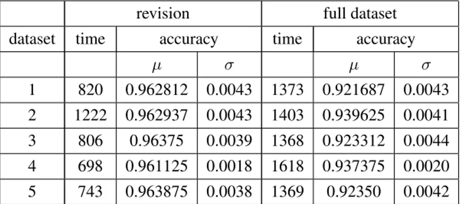
3.2 Revision compared to learning from full dataset for the hotel scenario . . . 47

3.3 Revision compared to learning from dataset for the auction scenario . . . 50

4.1 Excerpt from the interference matrix “sensitivity themes vs. power plants” in the Emilia-Romagna region . . . 55

6.1 Excerpt of the services with average service time . . . 90

6.2 Comparison of search strategies and hand-made solution (ECLiPSe). . . 100

(12)

(13)

1 Introduction

Computational Sustainability is an interdisciplinary field whose aim is to apply techniques from computer science, information science, operations research, applied mathematics, and statistics for balancing environmental, economic, and societal needs for sustainable development (i.e., using the words of the 1983 United Nations Brundtland Commission, development that meets the needs of the present generation without compromising the ability of future generations to meet their own needs) (2).

The focus is developing computational and mathematical models and methods for decision making concerning the management and allocation of resources in order to help solve some of the most challenging problems related to sustainability.

In this thesis we present various problems related to the domain of Computational Sustain-ability, on a broad spectrum which encompasses several of its critical aspects: energy efficiency, water management, limiting greenhouse gas emissions and fuel consumption.

We contribute towards their solution addressing them by means of Logic Programming (LP) and Constraint Programming (CP), which are paradigms from Artificial Intelligence of proven theoretical and practical solidity.

LP and CP offer many advantages under the point of view of declarativeness and flexi-ble expressivity, which are crucial in an area such as Computational Sustainability, where the scenario is often dynamic and faceted and where problem specifics have to be gathered from different domains of expertise often difficult to formalize in a straightforward way. The rapid prototyping features of LP and CP allow one to deliver working models in short time, test them on scaled-down instances and get quick feedback from the experts of the domain in order to

(14)

1. INTRODUCTION

(incrementally) refine the model and improve efficiency in a second stage on top of the existent implementation.

This pattern strongly inspired the approach to the problems described in this thesis, which were proposed by experts of the respective domains (such as environmental agencies, hydraulic engineers, human resource departments) and tested on the real data instances they provided. The results are encouraging and show the aptness of the chosen methodologies and approaches. The overall aim of this work is twofold: both to address real world problems in order to achieve practical results and to get from the application of LP and CP technologies to complex scenarios feedback and directions useful for their improvement.

Publications

Papers containing part of the work described in this thesis were presented in various venues:

Conferences and book chapters:

M. Cattafi, E. Lamma, F. Riguzzi, and S. Storari. Incremental declarative pro-cess mining. In N. T. Nguyen and E. Szczerbicki, editors, Smart Information and Knowledge Management: Advances, Challenges, and Critical Issues, volume 260 of Studies in Computational Intelligence, pages 103–127. Springer, Heidelberg, Germany, 2009.(3)

M. Alberti, M. Cattafi, F. Chesani, M. Gavanelli, E. Lamma, M. Montali, P. Mello, and P. Torroni. Integrating abductive logic programming and description logics in a dynamic contracting architecture. Web Services, IEEE International Conference on 254–261, 2009.(4)

Journals:

M. Alberti, M. Cattafi, F. Chesani, M. Gavanelli, E. Lamma, P. Mello, M. Montali, and P. Torroni. A Computational Logic Application Framework for Service Dis-covery and Contracting. International Journal of Web Services Research, 8(3):1-25, July-September 2011 (5).

M. Cattafi, M. Gavanelli, M. Milano and P. Cagnoli. Sustainable biomass power plant location in the Italian Emilia-Romagna region. ACM Transactions on Intelli-gent Systems and Technology, 2(4), July 2011 (6).

(15)

M. Cattafi, M. Gavanelli, M. Nonato, S. Alvisi, and M. Franchini. Optimal place-ment of valves in a water distribution network with CLP(FD). Theory and Practice of Logic Programming, 11(4-5):731-747, 2011. Best paper award at the 27th In-ternational Conference on Logic Programming (ICLP 2011)(7).

Synopsis

This thesis is organized as follows. We first provide some preliminaries about Logic Program-ming and Constraint ProgramProgram-ming in Chapter 2. In Chapter 3 we present a Computational Logic framework whose aim is to ease the complexity of Service Oriented Architectures, a paradigm which can give a considerable contribution in terms of reducing energy consumption and greenhouse gas emissions of data centres. Energy and greenhouse emissions are also the subject of Chapter 4, this time on the side of energy production from biomass. Some kinds of biomass are a promising source of renewable and low carbon footprint energy but careful assessment of their supply context is necessary in order not to deplete the potential advantages. Chapter 5 is dedicated to another fundamental aspect of sustainability: water and its careful distribution by design of (topologically) robust networks. In Chapter 6 focus is on societal needs and their balance with environmental and economic aspects, the context being home health care and the challenges it poses. Finally, in Chapter 7 we conclude and suggest some future work.

(16)

(17)

2 Preliminaries

2.1 Logic Programming

A first order alphabet Σ is a set of predicate symbols and function symbols (or functors) to-gether with their arity. A term is either a variable or a functor applied to a tuple of terms of length equal to the arity of the functor. If the functor has arity 0 it is called a constant. An atom is a predicate symbol applied to a tuple of terms of length equal to the arity of the predicate. A literal is either an atom a or its negation ¬a. In the latter case it is called a negative literal. In logic programming, predicate and function symbols are indicated with alphanumeric strings starting with a lowercase character while variables are indicated with alphanumeric strings starting with an uppercase character.

A clause is a formula C of the form

h1∨ . . . ∨ hn← b1, . . . , bm

where h1, . . . , hnare atoms and b1, . . . , bmare literals, whose separation by means of commas

represents a conjunction. A clause can be seen as a set of literals, e.g., C can be seen as {h₁, . . . , hn, ¬b1, . . . , ¬bm}.

In this representation, the disjunctions among the elements of the set are left implicit.

Which form of a clause is used in the following will be clear from the context. h1∨ . . . ∨ hn

is called the head of the clause and b1, . . . , bm is called the body. We will use head(C) to

indicate either h1 ∨ . . . ∨ hn or {h1, . . . , hn}, and body(C) to indicate either b1, . . . , bm or

(18)

2. PRELIMINARIES

called a fact. When n = 1, C is called a program clause. When n = 0, C is called a goal. The conjunction of a set of literals is called a query. A clause is range restricted if all the variables that appear in the head appear as well in the body.

A theory P is a set of clauses. A normal logic program P is a set of program clauses. A term, atom, literal, goal, query or clause is ground if it does not contain variables. A substitutionθ is an assignment of variables to terms: θ = {V1/t1, . . . , Vn/tn}. The application

of a substitution to a term, atom, literal, goal, query or clause C, indicated with Cθ, is the replacement of the variables appearing in C and in θ with the terms specified in θ.

The Herbrand universe HU(P ) is the set of all the terms that can be built with function

symbols appearing in P . The Herbrand base HB(P ) of a theory P is the set of all the ground

atoms that can be built with predicate and function symbols appearing in P . A grounding of a clause C is obtained by replacing the variables of C with terms from HU(P ). The grounding

g(P ) of a theory P is the program obtained by replacing each clause with the set of all of its groundings. A Herbrand interpretation is a set of ground atoms, i.e. a subset of HB(P ). In the

following, we will omit the word ‘Herbrand’.

Let us now define the truth of a formula in an interpretation. Let I be an interpretation and φ a formula, φ is true in I, written I |= φ if

• a ∈ I, if φ is a ground atom a;

• a 6∈ I, if φ is a ground negative literal ¬a; • I |= a and I |= b, if φ is a conjunction a ∧ b; • I |= a or I |= b, if φ is a disjunction a ∨ b;

• I |= ψθ if φ = ∀Xψ for all θ that assign a value to all the variables of X; • I |= ψθ if φ = ∃Xψ for a θ that assigns a value to all the variables of X. A clause C of the form

h1∨ . . . ∨ hn← b1, . . . , bm

is a shorthand for the formula

∀Xh₁∨ . . . ∨ h_n← b₁, . . . , bm

where X is a vector of all the variables appearing in C. Therefore, C is true in an interpretation I iff, for all the substitutions θ grounding C, if I |= body(C)θ then I |= head(C)θ, i.e., if

(19)

2.2 Inductive Logic Programming

(I |= body(C)θ) → (head(C)θ ∩ I 6= ∅). Otherwise, it is false. In particular, a program rule is true in an interpretation I iff, for all the substitutions θ grounding C, (I |= body(C)θ) → h ∈ I.

A theory P is true in an interpretation I iff all of its clauses are true in I and we write I |= P.

If P is true in an interpretation I we say that I is a model of P . It is sufficient for a single clause of a theory P to be false in an interpretation I for P to be false in I.

For normal logic programs, we are interested in deciding whether a query Q is a logical consequence of a theory P , expressed as

P |= Q.

This means that Q must be true in a model M (P ) of P that is assigned to P as its meaning by one of the semantics that have been proposed for normal logic programs (e.g. (8, 9, 10)).

For theories, we are interested in deciding whether a given theory or a given clause is true in an interpretation I. This can be achieved with the following procedure (11). The truth of a range restricted clause C on a finite interpretation I can be tested by asking the goal ?-body(C), ¬head(C) against a database containing the atoms of I as facts. By ¬head(C) we mean ¬h1, . . . , ¬hm. If the query fails, C is true in I, otherwise C is false in I.

In some cases, we are not given an interpretation I completely but we are given a set of atoms J and a normal program B as a compact way of indicating the interpretation M (B ∪ J ). In this case, if B is composed only of range restricted rules, we can test the truth of a clause C on M (B ∪J ) by running the query ?-body(C), ¬head(C) against a Prolog database containing the atoms of J as facts together with the rules of B. If the query fails, C is true in M (B ∪ J ), otherwise C is false in M (B ∪ J ).

2.2 Inductive Logic Programming

Inductive Logic Programming (ILP) (12) is a research field at the intersection of Machine Learning and Logic Programming. It is concerned with the development of learning algorithms that adopt logic for representing input data and induced models. Recently, many techniques have been proposed in the field and they were successfully applied to a variety of domains. Logic proved to be a powerful tool for representing the complexity that is typical of the real

(20)

2. PRELIMINARIES

world. In particular, logic can represent in a compact way domains in which the entities of interest are composed of subparts connected by a network of relationships. Traditional Ma-chine Learning is often not effective in these cases because it requires input data in the flat representation of a single table.

The problem that is faced by ILP can be expressed as follows: Given:

• a space of possible theoriesH; • a set E+_{of positive example;}

• a set E−of negative examples; • a background theory B. Find a theory H ∈H such that;

• all the positive examples are covered by H • no negative example is covered by H

If a theory does not cover an example we say that it rules the example out so the last condition can be expressed by saying the “all the negative examples are ruled out by H”.

The general form of the problem can be instantiated in different ways by choosing appro-priate forms for the theories in input and output, for the examples and for the covering relation. In the learning from entailment setting, the theories are normal logic programs, the ex-amples are (most often) ground facts and the coverage relation is entailment, i.e., a theory H covers an example e iff

H |= e.

In the learning from interpretations setting, the theories are composed of clauses, the ex-amples are interpretations and the coverage relation is truth in an interpretation, i.e., a theory H covers an example interpretation I iff

I |= H.

Similarly, we say that a clause C covers an example I iff I |= C.

We concentrate on learning from interpretation so we report here the detailed definition: Given:

(21)

• a space of possible theoriesH; • a set E+_{of positive interpretations;}

• a set E−_{of negative interpretations;}

• a background normal logic program B. Find a theory H ∈H such that;

• for all P ∈ E+_{, H is true in the interpretation M (B ∪ P );}

• for all N ∈ E−, H is false in the interpretation M (B ∪ N ).

The background knowledge B is used to encode each interpretation parsimoniously, by storing separately the rules that are not specific to a single interpretation but are true for every interpretation.

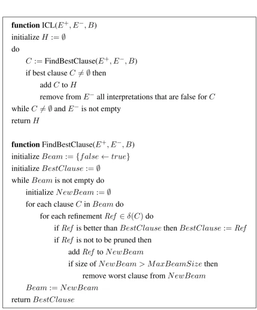
The algorithm ICL (13) solves the above problem. It performs a covering loop (function ICL in Figure 2.1) in which negative interpretations are progressively ruled out and removed from the set E−. At each iteration of the loop a new clause is added to the theory. Each clause rules out some negative interpretations. The loop ends when E−is empty or when no clause is found.

The clause to be added in every iteration of the covering loop is returned by the procedure FindBestClause (Figure 2.1). We look for clauses that cover as many positive interpretations as possible and rule out as many negative interpretations as possible. Starting from the clause f alse ← true, that rules out all the negative interpretations but also all the positive ones, the search gradually refines it. The algorithm is based on a beam search: the beam is a (finite) pool of candidate partial clauses to refine. At each iteration the best one, according to a certain heuristic, is selected and the worst one, according to the same criterion, is discarded if the beam is full. We use notation p( |C) for the probability that an example interpretation is classified as negative given that it is ruled out by the clause C. This probability can be a suitable heuristic and it is computed as the number of ruled out negative interpretations over the total number of ruled out interpretations (positive and negative). The refinements of a clause are obtained by generalization. A clause C is more general than a clause D if the set of interpretations covered by C is a superset of those covered by D. This is true if D |= C. However, using logical implication as a generality relation is impractical because of its high computational cost. Therefore, the syntactic relation of θ-subsumption is used in place of implication: D

(22)

2. PRELIMINARIES

function ICL(E+, E−, B) initialize H := ∅

do

C := FindBestClause(E+_{, E}−_{, B)}

if best clause C 6= ∅ then add C to H

remove from E−all interpretations that are false for C while C 6= ∅ and E−is not empty

return H

function FindBestClause(E+, E−, B) initialize Beam := {f alse ← true} initialize BestClause := ∅

while Beam is not empty do initialize N ewBeam := ∅ for each clause C in Beam do

for each refinement Ref ∈ δ(C) do

if Ref is better than BestClause then BestClause := Ref if Ref is not to be pruned then

add Ref to N ewBeam

if size of N ewBeam > M axBeamSize then remove worst clause from N ewBeam Beam := N ewBeam

return BestClause

(23)

θ-subsumes C (written D ≥ C) if there exist a substitution θ such that Dθ ⊆ C. If D ≥ C then D |= C and thus C is more general than D. The opposite, however, is not true, so θ--subsumption is only an approximation of the generality relation. For example, let us consider the following clauses:

C1 = accept(X) ← true

C2 = accept(X) ∨ refusal (X) ← true

C3 = accept(X) ← invitation(X)

C4 = accept(alice) ← invitation(alice)

Then C1 ≥ C2, C1 ≥ C3 but C2 6≥ C3, C3 6≥ C2 so C2 and C3 are more general than C1,

while C2and C3are not comparable. Moreover C1 ≥ C4, C3 ≥ C4but C2 6≥ C4and C46≥ C2

so C4is more general than C1and C3while C2and C4are not comparable.

From the definition of θ-subsumption, it is clear that a clause can be refined (i.e. general-ized) by applying one of the following two operations on a clause

• adding a literal to the (head or body of the) clause • applying a substitution to the clause.

FindBestClause computes the refinements of a clause by applying one of the above two op-erations. Let us call δ(C) the set of refinements so computed for a clause C. The clauses are thus gradually generalized until a clause is found that covers all (or most of) the positive interpretations while still ruling out some negative interpretations.

The literals that can possibly be added to a clause are specified in the language bias, a collection of statements in an ad hoc language that prescribe which refinements have to be considered. Two languages are possible for ICL:DLABand rmode (see (14) for details). Given

a language bias which prescribes that the body literals must be chosen among {invitation(X)} and that the head disjuncts must be chosen among {accept(X), refusal (X)}, an example of refinements sequence performed by FindBestClause is the following:

f alse ← true accept(X) ← true

accept(X) ← invitation(X)

accept(X) ∨ refusal (X) ← invitation(X)

The refinements of clauses in the beam can also be pruned: a refinement is pruned if it is not statistical significant and if it cannot produce a value of the heuristic function larger than that of the best clause. As regards the first type of pruning, a statistical test is used, while as regards

(24)

2. PRELIMINARIES

the second type of pruning, the best refinement that can be obtained is a clause that covers all the positive examples and rules out the same negative examples as the original clause.

When a new clause is returned by FindBestClause, it is added to the current theory. The negative interpretations that are ruled out by the clause are ruled out as well by the updated theory, so they can be removed from E−.

2.2.1 Incremental Inductive Logic Programming

The learning framework presented in Section 2.2 assumes that all the examples are provided to the learner at the same time and that no previous model exists for the concepts to be learned. In some cases, however, the examples are not all known at the same time and an initial theory may be available. When a new example is obtained, one approach consists of adding the example to the previous training set and learning a new theory from scratch. This approach may turn out to be too inefficient, especially if the amount of previous examples is very high. An alternative approach consists in revising the existing theory to take into account the new example, in order to exploit as much as possible the computation already done. The latter approach is called Theory Revision and can be described by the following definition:

Given:

• a space of possible theoriesH; • a background theory B

• a set E+_{of previous positive example;}

• a set E−of previous negative examples; • a theory H that is consistent with E+_{and E}−

• a new example e.

Find a theory H0 ∈H such that;

• H0_{is obtained by applying a number of transformations to H}

• H0covers e if e is a positive example, or • H0_{does not cover e if e is a negative example.}

(25)

2.3 Abductive Logic Programming and theSCIFF system

Theory Revision has been extensively studied in the learning from entailment setting of Induc-tive Logic Programming. In this case, examples are ground facts, the background theory is a normal logic program and the coverage relation is logical entailment. Among the systems that have been proposed for solving such a problem are: RUTH (15), FORTE (16) and Inthelex (17)

All these systems perform the following operations:

• given an uncovered positive example e, they generalize the theory T so that it covers it • given a covered negative example e, they specialize the theory T so that it does not cover

it

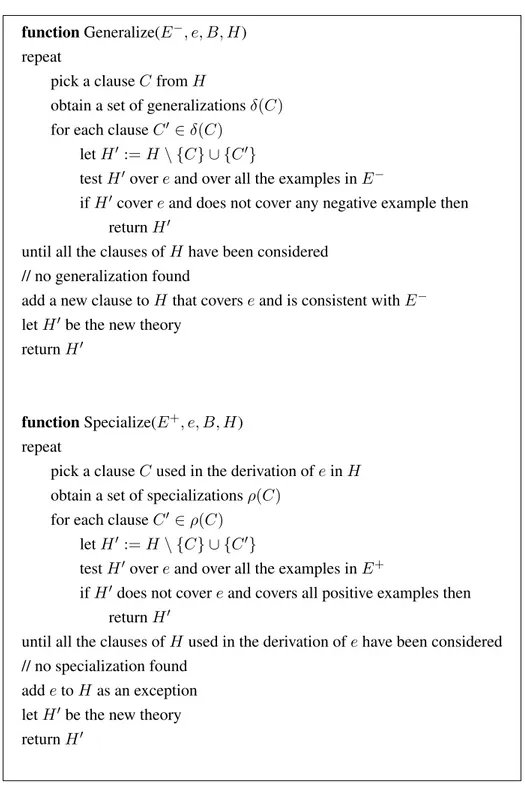
As an example of an ILP Theory Revision system, let us consider the algorithm of Inthelex that is shown in Figure 2.2. Function Generalize is used to revise the theory when the new example is positive. Each clause of the theory is considered in turn and is generalized. The resulting theory is tested to see whether it covers the positive example. Moreover, it is tested on all the previous negative examples to ensure that the clause is not generalized too much. As soon as a good refinement is found it is returned by the function.

Function Specialize is used to revise the theory when the new example is negative. Each clause of the theory involved in the derivation of the negative example is considered in turn and is specialized. The resulting theory is tested to see whether it rules out the negative example. Moreover, it is tested on all the previous positive examples to ensure that the clause is not specialized too much. As soon as a good refinement is found it is returned by the function.

While various systems exist for Theory Revision in the learning from entailment setting, to the best of our knowledge no algorithm has been proposed for Theory Revision in the learning from interpretation setting.

2.3 Abductive Logic Programming and the

SCIFF system

Abductive Logic Programming (18) is useful in a number of situations involving reasoning with incomplete knowledge and dynamic occurrence of events. SCIFF (19) is an extension of the IFF abductive language and proof-procedure (20). Its main motivations originate from the domain of agent interaction where the definition of agent communication languages and proto-cols, their semantic characterization and their verification are key issues. Its aim is to specify in a declarative but intensional way what are “admissible interactions” among agents, and to

(26)

2. PRELIMINARIES

function Generalize(E−, e, B, H) repeat

pick a clause C from H

obtain a set of generalizations δ(C) for each clause C0 ∈ δ(C)

let H0 := H \ {C} ∪ {C0}

test H0over e and over all the examples in E−

if H0cover e and does not cover any negative example then return H0

until all the clauses of H have been considered // no generalization found

add a new clause to H that covers e and is consistent with E− let H0be the new theory

return H0

function Specialize(E+, e, B, H) repeat

pick a clause C used in the derivation of e in H obtain a set of specializations ρ(C)

for each clause C0 ∈ ρ(C) let H0 := H \ {C} ∪ {C0}

test H0over e and over all the examples in E+

if H0does not cover e and covers all positive examples then return H0

until all the clauses of H used in the derivation of e have been considered // no specialization found

add e to H as an exception let H0be the new theory return H0

(27)

provide a computational tool to decide whether a given interaction is admissible (verification of compliance).

An Abductive Logic Program (ALP) is defined as the triplet hKBS,A, ICi, where KBS

is a logic program in which the clauses can contain special atoms, that belong to the setA and are called abducibles. Such atoms are not defined by means of clauses in the KBS, and, as

such, they cannot be proved: their truth value can be only hypothesized. In order to avoid un-constrained hypotheses, a set of integrity constraints (IC) must always be satisfied. Integrity constraints, in SCIFF are in the form of implications, and can relate abducible literals, de-fined literals, as well as constraints with Constraint Logic Programming semantics (see Section 2.4.6).

Given an abductive logic program T = hP, Ab, ICi and a formula G, the goal of abduction is to find a (possibly minimal) set of ground atoms ∆ (abductive explanation) in predicates in Ab which, together with P , “entails” G, i.e., P ∪ ∆ |= G, and such that P ∪ ∆ “satisfies” IC, e.g. P ∪ ∆ |= IC (see (18) for other possible notions of integrity constraint “satisfaction”). Here, the notion of “entailment” |= depends on the semantics associated with the logic program P (there are many different choices for such semantics (21)).

2.3.1 Syntax of theSCIFF language

The SCIFF language is composed of entities for expressing events and expectations about eventsand relationships between events and expectations.

Eventsare the abstractions used to represent the actual behaviour. Definition 1 An event is an atom:

• with predicate symbol H;

• whose first argument is a ground term; and • whose second argument is an integer.

Intuitively, the first argument is meant to represent the description of the happened event, ac-cording to application-specific conventions, and the second argument is meant to represent the time at which the event has happened.

Example 1

(28)

2. PRELIMINARIES

says that alice asked bob his phone_number with a query_ref message, in the context identified by dialog_id, at time 10.

A negated event is a negative literal not H(. . . , . . .). We will call history a set of happened events, and denote it with the symbol HAP.

Expectations are the abstractions used to represent the desired events from an external viewpoint (cannot be enforced, only expected to be as one would like them to be).

Expectations are of two types:

• positive: representing some event that is expected to happen; • negative: representing some event that is expected not to happen. Definition 2 A positive expectation is an atom:

• with predicate symbol E;

• whose first argument is a term; and

• whose second argument is a variable or an integer.

Intuitively, the first argument is meant to represent an event description, and the second argu-ment is meant to tell for what time the event is expected (which should not be confused with the time at which the expectation is generated, which is not modeled by theSCIFF’s declarative semantics). Expectations may contain variables, which leaves the expected event not com-pletely specified. Variables in positive expectations are always existentially quantified: if the time argument is a variable, for example, this means that the event is expected to happen at any time.

Example 2 The atom

E(tell(bob, alice, inform(phone_number, X), dialog_id), Ti) (2.2)

says that bob is expected to inform alice that the value for the piece of information identified by phone_number is X, in the context identified by dialog_id. Such (inform) event should happen at some timeTito fulfil the expectation.

A negated positive expectation is a positive expectation with the explicit negation operator ¬ applied to it. Variables in negated positive expectations are quantified as those in positive expectations.

(29)

Definition 3 A negative expectation is an atom:

• with predicate symbol EN;

• whose first argument is a term; and

• whose second argument is a variable or an integer.

Intuitively, the first argument is meant to represent an event description, and the second ar-gument is meant to tell in which time points the event is expected not to happen. As well as positive expectations, negative expectations may contain variables which are typically univer-sally quantified: for example, if the time argument is a variable, then the event is expected not to happen at all times.

Example 3 The atom

EN(tell(bob, alice, refuse(phone_number), dialog_id), Tr) (2.3)

means that bob is expectednot to refuse to alice his phone_number, in the context identified by dialog_id, atany time.

A negated negative expectation is a negative expectation with the explicit negation operator ¬ applied to it. Variables in negated negative expectations are quantified as those in negative expectations.

Is is worth noticing that

¬E(tell(bob, alice, refuse(phone_number), dialog_id), T_r)

is different from

EN(tell(bob, alice, refuse(phone_number), dialog_id), Tr)

. The intuitive meaning of the former is: no refuse is expected by Bob (if he does, we simply did not expect him to), whereas the latter has a different, stronger meaning: it is expected that Bob does not utter refuse (by doing so, he would frustrate our expectations).

(30)

2. PRELIMINARIES

2.3.1.1 Syntax with explicit quantifiers

AlthoughSCIFF offers a very rich, flexible and transparent (i.e., implicit) quantification of vari-ables, which keeps the language neat and simple, and makes it suitable to express interaction protocols in an intuitive way, in some contexts it can be useful to explicit the quantifiers.

ICs can thus be expressed as follows:

Body → ∃(ConjP1) ∨ . . . ∨ ∃(ConjPn) ∨ ∀¬(ConjN1) ∨ . . . ∨ ∀¬(ConjNm) (2.4)

where Body, ConjPi i = 1, . . . , n and ConjNj j = 1, . . . , m are, as in the conjunctions

of literals built over event atoms, over predicates defined in the background or over built-in predicates such as ≤, ≥, . . .. The variables appearing in the body are implicitly universally quantified with scope the entire formula. The quantifiers in the head apply to all the variables appearing in the conjunctions and not appearing in the body.

We will use Body(C) to indicate Body and Head(C) to indicate the formula ∃(ConjP1)∨

. . .∨∃(ConjPn)∨∀¬(ConjN1)∨. . .∨∀¬(ConjNm) and call them respectively the body and

the head of C. We will use HeadSet(C) to indicate the set {ConjP1, . . . , ConjPn, ConjN1, . . . , ConjNm}.

Body(C), ConjPii = 1, . . . , n and ConjNj j = 1, . . . , m will be sometimes interpreted

as sets of literals, the intended meaning will be clear from the context. We will call P conjunc-tioneach ConjPi for i = 1, . . . , n and N conjunction each ConjNj for j = 1, . . . , m. We

will call P disjunct each ∃(ConjPi) for i = 1, . . . , n and N disjunct each ∀¬(ConjNj) for

j = 1, . . . , m.

An example of an IC written with explicit quantifiers is: a(bob, T ), T < 10

→∃(b(alice, T 1), T < T 1) ∨

∀¬(c(mary, T 1), T < T 1, T 1 < T + 10)

(2.5)

IC (2.5) means: if bob has executed action a at a time T < 10, then alice must execute action b at a time T 1 later than T or mary must not execute action c for 9 time units after T . The disjunct ∃(b(alice, T 1), T < T 1) stands for ∃T 1(b(alice, T 1), T < T 1) and the disjunct ∀¬(c(mary, T 1), T < T 1, T 1 < T + 10) stands for ∀T 1¬(c(mary, T 1), T < T 1, T 1 < T + 10).

(31)

2.4 Constraint Satisfaction Problems

2.4.1 Definition

Many problems in Artificial Intelligence can be considered as instances of Constraint Satisfac-tion Problems.

Definition 4 A Constraint Satisfaction Problem (CSP) is a triple P = hX, D, Ci where X = {X1, X2, . . . , Xn} is a set of unknown variables, D = {D1, D2, . . . , Dn} is a set of domains

andC = {c1, . . . , cm} is a set of constraints. Each cl(Xi1, . . . , Xik) is a relation, i.e., a

subset of the Cartesian product of the involved variablesDi1 × · · · × Dik. An assignment

A = {X1 7→ d1, . . . , Xn7→ dn} (where d1 ∈ D1, . . . , dn∈ Dn) is a solution iff it satisfies all

the constraints.

If all the constraints in a CSP are unary or binary (involve at most two variables), we have a binary CSP. Binary CSPs are often represented as graphs: each variable is a node and each constraint is an arc that links the involved variables.

Applications include various domains: scheduling, planning, logistics, timetabling, artifi-cial vision, molecular biology, etc (22, 23, 24, 25, 26, 27, 28).

2.4.2 Algorithms

In general, the tasks posed in the constraint satisfaction problem paradigm are computationally intractable (NP-hard). Various types of algorithms have been proposed to solve Constraint Sat-isfaction Problems; an exhaustive survey is beyond the scope of this thesis. A good introduction is given in (29).

2.4.3 Consistency Techniques

In order to reduce the complexity of looking for a solution of a CSP, domain values that are provably not part of any solutions can be deleted (domain filtering) testing consistency. Definition 5 A unary constraint c(Xi) is Node-Consistent iff ∀v ∈ Di, v ∈ c(Xi); i.e., each

valuev belonging to the domain of variable Xiis consistent.

Definition 6 A binary constraint c(Xi, Xj) is Arc-Consistent iff ∀v ∈ Di ∃u ∈ Dj such that

(v, u) ∈ c(Xi, Xj) and vice-versa. In other words, for each value v belonging to the domain

of variableXithere exists a valueu in the domain of Xj that is consistent withv and for each

(32)

2. PRELIMINARIES

procedure REVISE(Xi, Xj)

DELETE ← false; for each v in Dido

if there is no such u in Dj such that (u, v) is consistent,

then delete v from Di; DELETE ← true; endif; endfor; return DELETE; end REVISE procedure AC-3

Q ← C % Set of all the constraints while not Q empty

select and delete any constraint c(Xk, Xm) from Q;

if REVISE(Xk, Xm) then

Q ← Q ∪ {c(Xi, Xk) such that c(Xi, Xk) ∈ C, i 6= k, i 6= m}

endif endwhile end AC-3

Figure 2.3: Algorithm AC-3

A Constraint network is Arc-Consistent if all the constraints are Arc-Consistent. Every binary CSP can be converted into an equivalent (i.e., with the same solution set) CSP which is Arc-Consistent. Many algorithms achieving Arc-Consistency have been proposed. All these al-gorithms are based on the following idea: if a binary constraint c(Xi, Xj) is not arc-consistent,

there will be a value v that is not supported. Supposing that v is in the domain of Xi, there

is no value in the domain of Xj that is consistent with v. In this case, v can be safely

re-moved from the domain of Xi. When we delete a value, we have a list of things that must

be re-considered. In AC-3 (30), that is often used because of its simple implementation, the list contains constraints (or, equivalently, arcs of the constraint graph). AC-3 is reported in Figure 2.3.

(33)

Other levels of consistency have been defined: Path-Consistency (31) and k-consistency (32, 33) achieve higher level of consistency, but they are more expensive. In most cases, Arc-Consistency is a good tradeoff, hence it is widely used.

If we deal with non-binary constraints (also called global constraints), Arc-Consistency can be extended:

Definition 7 An n-ary constraint c(X1, . . . , Xn) is Generalized Arc-Consistent (GAC) iff ∀v ∈

Di,∀j 6= i, ∃vkj ∈ Djsuch that(vk1, . . . , vki−1, vi, vki+1, . . . , vkn) ∈ c(X1, . . . , Xn).

Even when a non-binary CSP can be converted into a binary one (34), the use of global constraints is often beneficial. The model can be expressed in a more declarative, clear and concise way, and propagation is usually stronger too.

2.4.4 Systematic Search Algorithms

Systematic search algorithms build a search tree and explore it to find a feasible assignment.

2.4.4.1 Backtracking

Backtracking (or Standard Backtracking, or Chronological Backtracking) (35) incrementally attempts to extend a partial solution that specifies consistent values for some of the variables, toward a complete solution, by repeatedly choosing a value for another variable consistent with the values in the current partial solution. We have a labelling phase and a test for consistency phase.

In the labelling phase an unassigned variable is chosen and assigned a value in its domain. In the test phase, the last assignment is checked for consistency with all the other variables that were assigned before. If an inconsistency is detected, the last assignment is undone, and another value is chosen.

2.4.4.2 Forward Checking

Forward Checking (FC) (36) is a commonly used algorithm for solving CSPs, because it is simple and effective. This algorithm interleaves a labelling phase and a propagation phase. In the labelling phase a tentative value v is assigned to a given variable X as in Standard Backtracking. In the propagation phase, unassigned variables connected to X are considered,

(34)

2. PRELIMINARIES

and all values inconsistent with v removed from the corresponding domains, so only consistent values remain.

When a domain becomes empty, we have a failure, and the algorithm (chronologically) backtracks.

2.4.5 Constraint Optimization Problems

In some cases, finding a feasible solution is not enough, and a preference between solutions must be expressed. This preference is usually given with a function, that maps solutions into a cost (for minimization problems) or to a profit (for maximization problems).

2.4.5.1 Definition

For our needs, we define the Constraint Optimization problem as follows:

Definition 8 A Constraint Optimization Problem (COP) is a pair Q = hP, gi such that P is a CSP andg : D1× · · · × Dn 7→ St(wherehSt, ≤i is a totally-ordered set) is a merit function

that maps each solution tuple into a value. A solutionA of P is also a solution of the COP iff @A0 solution ofP such that g(A) < g(A0).

We have thus a total order induced by the function f on the set of possible CSP solutions. We will consider a maximization problem, being straightforward the extension to minimization problems.

2.4.5.2 Algorithms

The usual algorithm for solving COPs is Branch-and-Bound (37).

Branch and Bound is a general search method; a possible description of Branch-and-Bound is as follows. The whole problem is divided into two or more subproblems, as in a tree-search. When we find a solution, we impose that the solution must not be worse than the current optimal solution. A sketch of the algorithm is presented in Figure 2.4.

The comparison between the current optimum and the value in each node of the search tree can be performed in different ways. In the original formulation, an Upper Bound must be computed in every node of the search tree; if the Upper Bound is worse than the current best, the branch can be pruned off, because it cannot lead to an improvement of the solution.

(35)

let CSP = hX, D, Ci, COP = (CSP, g)

let AP = {CSP } % Set of Active Problems CurSol = −∞ % Current best solution WhileAP 6= ∅

choose P ∈ AP , let P = hXp, Dp, Cpi

if P is inconsistent AP ← AP \ {P }

Else if P has only one solution Sp

% Add the constraintg(X) > f (Sp) to all the active problems

∀Q ∈ AP, Q = hXq, Dq, Cqi, Cq← Cq∪ {g(Xq) > g(Sp)}

letCurSol ← Sp

Else% Branch

Generate the set CP of children of P AP ← AP \ P ∪ CP

End While ReturnCurSol

Figure 2.4: B&B Algorithm

2.4.6 Constraint Logic Programming

Constraint Logic Programming is a class of programming languages at the intersection of Con-straint Solving and Logic Programming (38). The paradigm of Logic Programming, as shown in Section 2.1 is declarative and thus allows a separation between logic and control (39). The logicpart is responsible for correctness and describes information, given as facts and relations, which must be manipulated and combined to compute the desired result. The control part is responsible for efficiency, and embeds the strategies and control of the manipulations and com-binations. An ideal programming methodology would be first of all concerned with what is the desired result; then, if necessary, with efficiency, or how to obtain the result. In Prolog, the most common logic programming language, the logic is given by first order predicate logic and the control is based on SLD-resolution.

However, one drawback of Logic Programming is that the manipulated objects are uninter-preted structures and equality only holds between objects that are syntactically identical. So, for instance, 1 + 2 is a syntactic object that cannot unify with 3.

(36)

2. PRELIMINARIES

(40). It represents a class of declarative languages, CLP(C) which are parametric in the con-straint domainC. For example, C can be the set of real numbers, and we have the CLP(R) (41), or the Finite Domain sort, thus we have CLP(F D). Constraint Logic Programming gives an interpretation to some of the syntactic structures and replaces unification with constraint solving in the domain of the computation.

More formally, the constraint domainC contains the following components (42):

• The constraint domain signature Σ_C. It is a signature (i.e., a set of functions and predicate symbols) that represents the subset of the syntactic structures that are interpreted in the domainC.

• The class of constraintsL_C, which is a set of fist-order formulas.

• The domain of computationD_C, which is a Σ-structure that is the intended interpretation of the constraints. It consists of a set D and a mapping from the symbols in Σ_Cto the set D.

• The constraint theory,T_C, which is a Σ-theory that describes the logical semantics of the constraints.

• The solver, solv_C, which is a solver for L_C, i.e., a function that maps each formula to true, f alse or unknown, indicating that the set of constraints is satisfiable, unsatisfiable or that it cannot tell.

In this thesis, we will mainly refer to the F D and R sorts. In F D the domain of the computation can be any finite set of elements. One of the most important instances is the set of integers comprised between two values [−M ax.. + M ax]: in this case the signature contains the integers, plus operations like +, −, ∗, / and constraints like =, <, >, ≤, ≥ that are interpreted as in mathematics. In most CLP languages (43, 44, 45), the solver solvF Dis based

on (Generalized) Arc-Consistency.

There are various implementations of the R sort with different characteristics, we will mostly refer to the one presented in (46).

(37)

3 Computational Logic tools for Green

IT

3.1 Introduction

Service Oriented Architectures (SOA), exploiting the Internet as a means of communication, are emerging as a simple and effective paradigm for distributed application development. Het-erogeneous entities, in terms of hardware and software settings, can interoperate effectively following well established communication standards.

This ‘decentralization’ of software has proved not only to be beneficial under the point of view of software engineering but also with respect to sustainability. Computing requirements have risen sharply over the last years, and data centres have acquired a considerable and grow-ing impact in terms of energy consumption and carbon footprint. Accordgrow-ing to the American Environmental Protection Agency, data centers consumed 0.7% of total US electricity in 2000 and 1.5% in 2006, while the Department of Energy estimate for 2010 is around 3% (1).

SOA enables businesses to delegate tasks to specialized structures which can benefit of economies of scale and thus the whole system can use resources in a more flexible and efficient way. Some independent analyst firms have conducted quantitative studies in order to show that

“the growth of cloud computing will have a very significant positive effect on data center energy consumption. Few, if any, clean technologies have the capability to reduce energy expenditures and greenhouse gas production with so little business disruption. Software as a service, infrastructure as a service, and platform as a service are all inherently more efficient models than conventional alternatives, and

(38)

3. COMPUTATIONAL LOGIC TOOLS FOR GREEN IT

Figure 3.1: Model derived carbon emission savings enabled by cloud computing according to (1)

their adoption will be one of the largest contributing factors to the greening of enterprise IT.” (47).

According to one of the available reports, “US businesses with annual revenues of more than $1 billion can cut carbon emissions by 85.7 million metric tons annually by 2020 as a result of spending 69% of infrastructure, platform and software budgets on cloud services” (1), see also Figure 3.1.

However organizing software as a composition of services introduces elements of consider-able complexity related to the need to coordinate their interaction. Interoperability of services has a ‘syntactic’ aspect, which can be achieved by using standards and expressing interfaces of what types of data are taken in input and produced in output by services (48). But it needs to be accompanied by a ‘semantic’ one, with a formal specification of what the service ‘does’ and the technological intelligent tools to understand and elaborate them.

3.1.1 Semantic Web Services

Service providers can expose their policies, in order for potential customers to evaluate the fea-sibility of a fruitful interaction. Such an evaluation can be performed manually, if the service’s interface is bound not to change over time.

However, a more promising approach is for customers to choose the appropriate service provider at run-time, based on the service provider’s exposed policies.

This approach requires a reasoning engine that reasons on the provider and customer’s goals and policies, in order to devise a sequence of actions that lets both achieve their goals, while respecting their policies.

(39)

3.1 Introduction

In (49), Alberti et al. proposed a contracting architecture based on the SCIFF abductive logic framework presented in Section 2.3. In that work, the policies were expressed by means of integrity constraints, and the domain knowledge was expressed in SCIFF’s logic clauses. The sound and completeSCIFF proof procedure was employed to find, if possible, a course of action that was satisfactory for both.

However, in a practical perspective, we envisage a possible improvement in representing the domain specific knowledge exploiting the vast body of results from the Knowledge Repre-sentation field and, in particular, Description Logics. In this way, we can address the Ontology layer of the Semantic Web stack.

In this chapter, we propose an approach to letSCIFF access existing knowledge, expressed by means of an ontology: by interfacing SCIFF with ontological reasoners, distinguishing syntactically the ontology-related predicates and delegating their computation to the external reasoners.

This approach bears two main practical advantages: first, it makes the knowledge encoded in ontologies available toSCIFF, and second it takes advantage of the formal properties en-joyed by the existing ontological reasoners for the associated computational tasks, in particular concerning decidability and efficiency.

Moreover we deal with a dual aspect of contracting: learning and updating policies from existent interactions. This is a very important issue because policies can be rather complex and even experts of the domain can find it very difficult to express them in a formal language. The overall process can be very time-consuming and error-prone, while classification of an interaction as compliant (or not) with respect to the intended behaviour is usually easier.

Applying techniques inspired by Inductive Logic Programming (see Section 2.2) authors of (50) propose a framework for policy learning. We extend it in order to include the cases, often relevant in the dynamic domain of Web Services, in which policies are already partially specified and one wants to update them taking advantage of new available knowledge.

After recalling in Section 3.2 how Semantic Web Services contracting can be represented inSCIFF we show, in Section 3.3, how it could benefit of added ontological expressivity. We describe a possible implementation and its experimental evaluation in Sections 3.4.1 and 3.4.2 respectively.

In Section 3.5 we discuss in detail the problem of learning policies from histories of pre-vious interactions. After explaining how this knowledge can be represented in logic in Section 3.6, we present a framework designed to learn policies from such information (Section 3.7) and

(40)

its extension which is able to update policies when new knowledge is available (Section 3.8). The two approaches are compared in Section 3.9. In Section 3.10 we discuss related work in the field.

3.2 Contracting with

SCIFF

In this section, we briefly recall theSCIFF-based contracting framework (49).

A web service’s policy is defined, in theSCIFF language, as an abductive logic program (ALP). In particular, the integrity constraints can relate the web services’ information ex-changes with the expected input from peer web services. The possible relations can be of various types, and include temporal relations, such as deadlines, linear constraints, inequalities and disequalities, all defined by means of constraints. The definitions stated in this way are then used to make assumptions on the possible evolutions of the interaction.

3.2.1 A contracting scenario

In (49) theSCIFF framework is applied to contracting in an e-commerce scenario, which we extend here in order to demonstrate our approach to integration.

The two actors are eShop (which wants to sell a device) and alice (a potential customer for that device), each with policies expressed as SCIFF ICs. SCIFF is used as a reasoner in a component that acts as a mediator, considering the actors’ policies and trying to devise a course of action that will let both reach their goals. The two actors’ policies, expressed in SCIFF integrity constraints, are as follows.

(41)

3.2 Contracting withSCIFF

alice’s policy. “If the shop asks me to pay cash, I will, but if the shop asks me to pay by credit card, I will require evidence of the shop’s affiliation to the Better Business Bureau.“

H(tell(Shop, alice, ask(pay(Item, cc))), T a) → H(tell(alice, Shop, request_guar(BBB)), T rg)∧

E(tell(Shop, alice, give_guar(BBB)), T g) ∧ T g > T rg ∧ T rg > T a.

H(tell(Shop, alice, ask(pay(Item, cc))), T a)∧ H(tell(Shop, alice, give_guar(BBB)), T g) →

H(tell(alice, Shop, pay(Item, cc)), T p) ∧ T p > T a ∧ T p > T g.

H(tell(Shop, alice, ask(pay(Item, cash))), T a) → H(tell(alice, eShop, pay(Item, cash)), T r) ∧ T a < T r.

(3.1)

eShop’s policy. “If an acceptable customer requests an item from me, then I expect the cus-tomer to pay for the item with an acceptable means of payment. If the cuscus-tomer is not accept-able, I will inform him/her of the failure. If an acceptable customer pays with an acceptable means of payment, I will deliver the item. If a customer requests evidence of my affiliation to the Better Business Bureau (BBB), I will provide it.”

H(tell(Customer, eShop, request(Item)), T r) ∧ accepted_payment(How) →

accepted_customer(Customer) ∧ H(tell(eShop, Customer, ask(pay(Item, How))), T a)∧ E(tell(Customer, eShop, pay(Item, How)), T p) ∧ T p > T a ∧ T a > T r

∨ rejected_customer(Customer) ∧ H(tell(eShop, Customer, inf orm(f ail)), T i) ∧ T i > T r.

H(tell(Customer, eShop, pay(Item, How)), T p)

∧ accepted_customer(Customer) ∧ accepted_payment(How) → H(tell(eShop, Customer, deliver(Item)), T d) ∧ T d > T p.

H(tell(Customer, eShop, request_guar(BBB)), T rg) → H(tell(eShop, Customer, give_guar(BBB)), T g) ∧ T g > T rg.

(42)

The notion of acceptability for customers and payment methods from eShop’s viewpoint, defined by the accepted_customer/1 and accepted_payment/1 predicates, is defined in eShop’s knowledge base. In (49), only EU residents are accepted customers, as defined by the following clauses: accepted_customer(Customer):-resident_in(Customer, Location), accepted_destination(Location). rejected_customer(Customer):-resident_in(Customer, Location), not accepted_destination(Location). accepted_destination(european_union). accepted_payment(cc). accepted_payment(cash).

This knowledge is merged with that provided by the customer, for example

resident_in(alice,european_union).

so that in the resulting knowledge base, on whichSCIFF operates, accepted_customer(alice)is true.

However, this method would not work in case the customer declared

resident_in(alice,italy), as italy does not unify with european_union. One could, of course, add to the knowledge base accepted_destination/1 facts for all the current EU members, but such knowledge should be updated when new countries join the EU. In other cases, acceptability could be defined by a transitive, symmetric relation, which could introduce cycles in the knowledge base, possibly leading to loops.

3.3 Representing domain knowledge with ontologies

An alternative way to represent (part of) the domain specific knowledge is to use technology and concepts developed, with focus on this very purpose, in the Knowledge Representation field, and to rely, in particular, on ontologies. The W3C recommendation for ontology repre-sentation on the Web is the Web Ontology Language (OWL) (51) based on the well established semantics of Description Logics (52) and on XML and RDF syntax. Using OWL for domain

(43)

3.3 Representing domain knowledge with ontologies

Figure 3.2: A graphical representation of the ontology

knowledge representation improves expressiveness (with such features as stating sub-class re-lations, constructing classes on property restrictions or by set operators, defining transitive properties and so on) yet keeping decidability (if using OWL Lite or OWL DL) in a straight-forward and domain modeling-oriented notation. Moreover, since OWL is tailored for the Web, it provides support for expressing knowledge in distributed contexts (identified by URIs) and its recognized standard status is a warranty on interoperability and reuse issues. As a plus, it can be mentioned that community driven development of Semantic Web tools already provides good support for OWL ontology management tasks such as editing (53) also for not KR-skilled users.

For instance, in Fig. 3.2 we show a possible ontological representation of eShop’s policies concerning acceptable customers and means of payments, merged with alice’s own knowledge. The following OWL axiom says that the acceptedCustomer class is a subclass of the potentialCustomerclass, and that it is disjoint from the

(44)

3. COMPUTATIONAL LOGIC TOOLS FOR GREEN IT rejectedCustomerclass: <owl:Class rdf:about="#acceptedCustomer"> <rdfs:subClassOf rdf:resource="#potentialCustomer" /> <owl:disjointWith rdf:resource="#rejectedCustomer" /> </owl:Class>

The following fact states that cash is an instance of the acceptedPayment class:

<owl:Thing rdf:about="#cash">

<rdf:type rdf:resource="#acceptedPayment" /> </owl:Thing>

The following axiom declares the paysWith property:

<owl:ObjectProperty rdf:ID="paysWith">

<rdfs:domain rdf:resource="#potentialCustomer" /> <rdfs:range rdf:resource="#payment" />

</owl:ObjectProperty>

The following fact states that alice is an instance of italian, with value ae1254 for the paysWithproperty:

<owl:Thing rdf:about="#alice">

<rdf:type rdf:resource="#italian" /> <paysWith rdf:resource="#ae1254" /> </owl:Thing>

It can be noticed that the ontological notation for the KB makes it possible to infer that alice is European (and therefore an accepted customer) even if she just states being Italian, while if we had put resident_in(alice, italy) instead of resident_in(alice, europe)in the KB at the end of Sect. 3.2.1 she would not have been recognized as such.

Moreover, we defined a class premiumCustomer representing the accepted customers who pay with a credit card, and which we could use to add refinement to policies (for instance providing a faster delivery). Since alice is an accepted customer and pays with her credit card, the ontological reasoning allows to recognize her as a premiumCustomer.

(45)

3.4 Handling semantic knowledge withSCIFF

Figure 3.3: Integration architecture

3.4 Handling semantic knowledge with

SCIFF

In this section we describe our implementation of the SCIFF access to OWL ontologies. It should be noticed that even if OWL relies on the Open World Assumption, whenSCIFF comes to reasoning involving it, the logic programming peculiar Closed World Assumption is rein-troduced, thus assuming to have all (relevant) information on the domain available at that time and providing usual features such as negation as failure.

3.4.1 InterfacingSCIFF and ontological reasoners

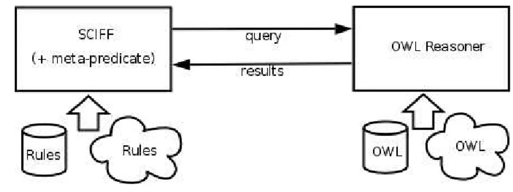
An external specific ontology-focused component interfaced with SCIFF can be, when nec-essary, queried in order to perform the actual ontological reasoning and give back results. As represented in Fig. 3.3, the architecture for this solution involves a Prolog meta-predicate which invokes the ontological reasoning on desired goals, an intercommunication interface from SCIFF to the external component (which incorporates a query and results translation schema) and the actual reasoning module. Both modules can access both local and networked knowledge.

Goals given to the meta-predicate are handled like suggested in (54) and (55) considering single arity predicates as “belongs to class (with same name of predicate)" queries and dou-ble arity ones as “are related by property (with same name of predicate)" queries. To reduce the overhead caused by external communication, our implementation of the meta-predicate provides a caching mechanism: it is first checked if a similar query (i.e., involving the same predicate) has been performed before and, only if not, the external reasoner is invoked and answers are cached by storing them as Prolog facts (by means of asserta/1}).The OWL reasoning module uses the Pellet (56) API, while the communication interface uses the Jasper

(46)

N Load time Query time Total

100 ∼ 0 ∼ 0 ∼ 0

500 1.0 ∼ 0 1.0

1000 1.0 ∼ 0 1.0

5000 2.0 1.2 3.2

10000 4.0 2.8 6.8

Table 3.1: Performance results (all times are in seconds, average over 50 runs)

Prolog-Java library (44). This solution enables access to the full OWL(-DL) expressivity, in-cluding features such as equivalence of classes and properties, transitive properties, declaration of classes on property restriction and property-based individual classification.

3.4.2 Experimental evaluation

The approach was tested successfully in simple reasoning scenarios, such as the one depicted in Fig. 3.2.

To assess its scalability, we experimented with randomly generated ontologies. Each ontol-ogy, composed of N classes, was built starting from its root node, and recursively attempting, for each node, five attempts of child generation, each with probability 1/3.

The reasoner was queried about the belonging of an entity to the hierarchy root class. We report in Tab. 3.1 the time spent for loading the ontology into the reasoner (i.e. the time spent for parsing ICs and loading the ontology into a persistent OWLOntology object) and for the actual query. The approach appears to scale reasonably (on PC equipped with an Intel Celeron 2.4 GHz CPU), the loading time is usually higher than the query time.

3.5 Learning and Updating Policies

We have shown how the possibility to express Web Service policies in formal languages and the use of Computational Logic tools to perform reasoning about their composition and coor-dination has great potential to ease the complexity of these operations, thus bringing the SOA scenario closer to a feasible extended adoption.

However, writing policies in a formal language is often a very complicated issue itself. Sometimes not enough knowledge about the domain is available, or the domain expert finds it difficult to express it formally.