The impact of varying per capita intensities of EU Funds on regional growth: Estimating dose response treatment effects through statistical matching

March 2016 Authors:

The impact of varying per capita

intensities of EU Funds on

regional growth: Estimating dose

response treatment effects

through statistical matching

FINAL REPORT

Work package 14d:

Propensity score matching

Ex post evaluation of Cohesion Policy programmes

2007-2013, focusing on the European Regional

Development Fund (ERDF) and the Cohesion Fund (CF)

April 2016

EUROPEAN COMMISSION

Directorate-General for Regional and Urban Policy Directorate A1 — Policy coordination

Unit A1.B2 — Evaluation and European Semester Contact: Kai Stryczynski

E-mail: REGIO_EVAL@ec.europa.eu European Commission

Directorate-General for Regional and Urban Policy

2016 EN

The impact of varying per capita

intensities of EU Funds on

regional growth: Estimating dose

response treatment effects

through statistical matching

FINAL REPORT

Work package 14d:

Propensity score matching

Ex post evaluation of Cohesion Policy programmes

2007-2013, focusing on the European Regional

Development Fund (ERDF) and the Cohesion Fund (CF)

LEGAL NOTICE

This document has been prepared for the European Commission however it reflects the views only of the authors, and the Commission cannot be held responsible for any use which may be made of the information contained therein.

More information on the European Union is available on the Internet (http://www.europa.eu).

Luxembourg: Publications Office of the European Union, 2016

ISBN 978-92-79-58513-5 doi: 10.2776/256991

© European Union, 2016

Reproduction is authorised provided the source is acknowledged.

Europe Direct is a service to help you find answers

to your questions about the European Union.

Freephone number (*):

00 800 6 7 8 9 10 11

(*) The information given is free, as are most calls (though some operators, phone boxes or hotels may charge you).

3

Table of Contents

Executive Summary ... 7

PART I ... 8

1.

RDD vs Matching for Regional-Level CIEs of EU Funds (EUF) ... 8

2.

Data (Task 1) ... 10

3.

Caveats and limitations of the data (Task 1) ... 11

4.

Sample sizes and descriptive statistics (Task 1) ... 12

4.1

Sample sizes of NUTS2 regions available for the analysis ... 12

4.2

Descriptive statistics on the balance of the pre-intervention covariates (X) between Obj.1 and

non-Obj.1 regions ... 13

5.

Methods: Propensity Score Matching estimation ... 22

5.1

Radius Matching estimators ... 22

5.2

Nearest Available Caliper Matching ... 23

5.3

Kernel Matching ... 24

5.4

PS estimation and common support ... 24

6.

Summary of the results (Task 1) ... 30

7.

Concluding remarks (Task 1) ... 34

PART II ... 35

8.

Data (Tasks 2-3) ... 35

8.1

Outcome variables (Y) ... 35

8.2

EU Funds (EUF) per-capita intensities ... 35

8.3

Control variables (X) ... 36

9.

Caveats and limitations of the data (Tasks 2-3) ... 38

10.

Sample sizes and descriptive statistics (Tasks 2-3) ... 40

10.1

Descriptive statistics on the value of the EU Funds (EUF) across the three programming periods

1994-99; 2000-06; 2007-13 (EU27) ... 40

10.2

EU Funds (EUF) in the EU-27 regions sorted by Objective1/Convergence Obj. status (years

1994-2010) ... 44

10.3

Descriptive statistics on the outcome variables of the analysis: GVA, gross-fixed capital formation

and employment rate ... 45

11.

Dynamic Propensity Score Matching (PSM) models for estimating the average impacts of the

highest intensity of the EU Funds (EUF) in the Objective 1/Convergence Obj. regions ... 52

12.

Generalised Propensity Score (GPS) and Propensity Score Matching (PSM) models for estimating

the impact of continuous and multiple categorical treatment intensities ... 53

4

13.

Summary of the results (Tasks 2 and 3) ... 60

14.

Concluding remarks (Tasks 2 and 3) ... 63

References ... 65

Annex 1: Task 1 - Technical Appendix ... 66

5

Table of figures

Table 1 : Sample sizes of NUTS2 regions by Eligibility Status (T=1 Obj.1; T=0 non-Obj.1) ... 13

Table 2 : Sample sizes of NUTS2 regions within ¼ SD from cut-off of Z (67.85% <Z >82.15%) ... 13

Table 3 : Sample sizes of NUTS2 regions within 1/2 SD from cut-off of Z (60.70% <Z >89.30%) ... 13

Table 4 : Pre-intervention differences in Xgrw between Obj.1 (treated) and non-Obj.1 regions (control) .... 14

Table 5 : Pre-intervention differences in Xlev between Obj.1 (treated) and non-Obj.1 regions (control) ... 15

Table 6 : Results from the PS Radius Matching estimators (preferred specifications with the best balancing

of the control variables) ... 30

Table 7 : Results from the PS Nearest Available estimators with Caliper (preferred specifications) ... 32

Table 8 : Results from the PS Kernel Matching estimators, Gaussian with bandwidth (preferred

specifications) ... 33

Table 9 : Total EU Funds (1=1 Million €) by country and by period ... 40

Table 10 : Total per-capita EU Funds (1=1 € / per capita) by country and by Programming period ... 41

Table 11 : Average annual per-capita EU Funds (1=1 € / per capita / per year) by country and by

Programming period ... 42

Table 12 : Pooled distribution of the NUTS2 annual per-capita EU Fund intensities in the three

programming periods (1=1€ / per capita / per year) ... 43

Table 13 : Total sum of EU Funds received by NUTS2 regions over the whole 1994-2010 period ... 44

Table 14 : Average intensity of the EU Funds (EUF) by Obj.1/Convergence Obj status ... 45

Table 15 : NUTS2 regions sorted by categories of intensities of the EU Funds (EUF) ... 45

Table 16 : Annual average changes of GVA, gross fixed capital formation and employment rate by categories

of EU Fund (EUF) intensities. Programming period 1994-99 ... 46

Table 17 : Annual average changes of GVA, gross fixed capital formation and employment rate by categories

of EU Fund (EUF) intensities. Programming period 2000-06 ... 47

Table 18 : Annual average changes of GVA, Gross fixed capital formation and Employment rate by

categories of EU Fund intensities. Programming period 2007-13(*) ... 47

Table 19 : Average annual growth by Obj.1/Conv. Obj status ... 51

Table 20 : Variable specifications of the Dynamic PSM model with binary treatment intensity (EU-27 regions,

1994-2013 periods) ... 52

Table 21 : Variable specifications of Models I -II ... 58

Table 22 : Variable specifications of Models III-IV ... 59

Table 23 : Impacts of EU Funds (EUF) on GVA growth. EU-27, 1994-2011 ... 60

Table 24 : Impacts of EU Funds (EUF) on Gross fixed capital formation growth. EU-27, 1994-2011 ... 61

Table 25 : Impacts of EU Funds (EUF) on employment rate changes. EU-27, 1994-2011 ... 62

Figure 1 : Pre-intervention annual % change in the employment rate (1=p.p.) plotted against values of Z

(per-capita GDP in 1988-90 in terms of % of EU mean) ... 16

Figure 2 : Pre-intervention annual % growth in GDP per-capita (1=p.p.) plotted against values of Z

(per-capita GDP level in 1988-90 in terms of % of EU mean) ... 16

Figure 3 : Pre-intervention annual % change in worker compensation (1=p.p.) plotted against values of Z

(per-capita GDP in 1988-90 in terms of % of EU mean) ... 17

Figure 4 : Pre-intervention annual % growth in per-capita fixed capital formation (1=p.p.) plotted against

values of Z (per-capita GDP level in 1988-90 in terms of % of EU mean) ... 17

6

Figure 5 : Pre-intervention annual % growth (1=1 p.p.) in labour productivity (GDP per-worker) plotted

against values of Z (per-capita GDP level in 1988-90 in terms of % of EU mean) ... 18

Figure 6 : Pre-intervention average level of employment rate (1=1%) plotted against values of Z (per-capita

GDP in 1988-90 in terms of % of EU mean) ... 19

Figure 7 : Pre-intervention average level of GDP per-capita (1=EUR) plotted against values of Z (per-capita

GDP level in 1988-90 in terms of % of EU mean) ... 19

Figure 8 : Pre-intervention average level of worker compensation (1=EUR) plotted against values of Z

(per-capita GDP in 1988-90 in terms of % of EU mean) ... 20

Figure 9 : Pre-intervention average level of per-capita fixed capital formation (1=EUR) plotted against values

of Z (per-capita GDP level in 1988-90 in terms of % of EU mean) ... 20

Figure 10 : Pre-intervention average level of labour productivity (GDP per-worker, 1=1 EUR) plotted against

values of Z (per-capita GDP level in 1988-90 in terms of % of EU mean) ... 21

Figure 11 : Boxplots of the PS distributions based on Xgrw (Growth-trends controls) [All Regions] ... 25

Figure 12 : Boxplots of the PS distributions based on three Xgrw (Growth-trend controls) and three Xlev

(Average-level controls). [All Regions] ... 26

Figure 13 : Boxplots of the PS distributions based on all Xgrw (Growth-trend controls) and Xlev

(Average-level controls). [All Regions] ... 26

Figure 14 : Boxplots of the PS distributions based on Xgrw (Growth-trends controls). [Regions close to the

cut-off of eligibility: Z within 1/4 SD away from the cut-off] ... 27

Figure 15 : Boxplots of the PS distributions based on three Xgrw (Growth-trend controls) and three Xlev

(Average-level controls). [Regions close to the cut-off of eligibility: Z within 1/4 SD away from the cut-off]

... 28

Figure 16 : Boxplots of the PS distributions based on all Xgrw (Growth-trend controls) and Xlev

(Average-level controls) ... 28

Figure 17: Avg. annual amount of per-capita EUF plotted against the avg. annual growth rate of per-capita

GVA, GFCF, and annual change of employment rate. Programming period 1994-99 ... 48

Figure 18 : Avg. annual amount of per-capita EUF plotted against the avg. annual growth rate of per-capita

GVA, GFCF, and annual change of employment rate. Programming period 2000-06 ... 49

Figure 19 : Avg. annual amount of per-capita EUF plotted against the avg. annual growth rate of per-capita

GVA, GFCF, and annual change of employment rate. Programming period 2007-13(*) ... 50

Figure 20 : Causality chain, from EU funds to desirable regional growth outcomes ... 53

Figure 21 : Trade-off between model dependence and impact identification power ... 54

7

Summary

As part of the Ex post evaluation of the 2007-2013 programming period of the European

Cohesion Policy this report deals with the impact of the varying per capita intensities of EU

funds on regional growth. The works was separated in three tasks. The first one focuses on the

analysis of how the intensity variation of EU structural funds affected regional growth in the

EU-15 regions in the 1994-2006 period. Task 2 deals with the impact of EU cohesion policy on

regional growth in the EU-27 regions. Task 3 is wider because it tackles the analysis of

cohesion policy effects for all European countries, considering data up to 2013. Thanks to

statistical methods impacts are estimated. The tasks involved using a counterfactual impact

evaluation design, implementing with propensity score matching (PSM) and generalized

propensity score matching (GPSM).

As concerns the Task1 of this project, there were two main objectives of the analysis. A)

Compare results obtained with a PSM approach to those from earlier RDD analysis research

(Pellegrini et al. 2013 and Becker et al. 2013) to highlight lessons that can be learned on the

data availability scenarios that make preferable to use of one method as supposed to the

other. B). Estimate different impacts for different levels of the per capita intensity of the EUF.

As mentioned in the technical offer, objective B) of the analysis can be achieved by

operationalizing the intensity level of the EUF either dichotomously (as implemented in

Pellegrini et al 2013) or with multiple categories of intensity levels (in discrete or continuous

terms, as implemented, at the NUTS3 level, in Becker et al. 2013). To enhance comparability

with the RDD work package, and because of serious reliability issues with the NUTS3 level

data, it was agreed with DG-regio to use NUTS2 level as the units of observation of the

analysis, instead of the NUTS3 level used by in Becker et al. 2013. Because of the choice to

focus on NUTS2 regions as units of observation, the overall sample size of the regions with

comparable pre-intervention characteristics is not large enough (at the EU15 level for the

1994-2006 period) to allow statistically significant estimations of a continuous or categorical

dose-response function. For this reason the Task 1 analyses presented in this report is

implemented entirely within the framework of the dichotomous difference in the degree of

intensity of the EUF adopted in Pellegrini et al 2013 (i.e. a binary treatment status variables

that distinguishes the higher per capita intensity of the EUF related with “Obj.1”/“Convergence

Obj” eligibility from the lower per-capita intensity related with the “non-Obj.1/Convergence

Obj.1 eligibility”). Thus, as indicated in the technical offer, the actual data availability scenario

and sample size considerations dictated the choice of the exact model that was used in the

Task 1 analysis.

Generalised Propensity Score Matching and propensity score matching estimators with multiple

categorical treatment status variables for the different intensities of the EUF were instead

applied to the analysis for the Tasks 2 and 3 of this projects. These tasks involve estimating

how varying per capita intensity of EUF affected regional growth, extending the analysis of

Task 1 to include the larger sample of EU-27 regions over the period 1994-2013 and

considering a larger number of outcome variables to include, employment growth and growth

of (per capita) gross fixed capital formation, in addition to the per capita regional growth of

GDP used in Task 1

_.

1 _{As mentioned in the technical offer, the list of outcome variables used for the analysis has been}

determined in agreement with DG-Regio based on the actual data availability for the entire list of NUTS2 regions considered in the analysis.

8

PART I

1.

RDD vs Matching for Regional-Level CIEs of EU Funds (EUF)

When adopting RDD for regional-level CIEs of structural and cohesion fund programmes, the

following considerations apply:

• The units of observation for the analysis (i.e. the EU regions) did not self-selected into

applicants and non-applicant for obtaining the former Obj.1 / Convergence Obj status:

such eligibility was based, by the most part on the GNI in PPS recorded by Eurostat. For

this reason, no obvious advantage of RDD versus other CIE methods exist due to the fact

that in RDD the treated units can be compared only with untreated units with the same

initial desire to be treated (while, with other CIE methods, the treated units can be

potentially compared with a general population of non-treated units, regardless of whether

or not they participated into the program application process). Thus applying RRD versus

other CIE methods does not guarantee any better controlling of the unobservable

confounding factors (i.e factors affecting the outcome variable a part from the treatment)

leading to the same desire to be treated.

• In set ups suitable for RDD, the more the forcing variable (determining the treatment

status of the units of observations) is a factor with a weak influence on the outcome

variable Y of the analysis (i.e. a “non-dominant” forcing variable), the more the treatment

assignment process mimic an actual randomization also away from the cut-off point. This

bears an important consequence: The more the forcing variable does not constitute a

“dominant” confounding factor, the larger is the band across the cut-off point in which

conditions similar to a randomized experiment apply.

• Since RDD mimics a block randomization within the neighbourhoods of the cut-off point, in

the presence of small samples and of a “non-dominant” forcing variable, it has to checked

whether or not the sample of treated and non-treated units in the neighbourhood of the

cut-off point are indeed balanced with regards to the other relevant confounding factors

(different from the forcing variable). As widely discussed in the literature, this is common

wisdom in the field of randomized experiments: with small samples, unbalanced

compositions can happen and the randomization process has to be repeated or

implemented as block randomization with regards to all the major confounding factors.

• In the presence of small samples, the more “dominant” is the forcing variable, the less it is

necessary to check whether or not the treated and non-treated units in the neighbourhood

of the cut-off are balanced with regard to other confounding factors (this is because similar

levels of a “dominant” forcing variable ensure per-se an overall balance between treated

and non-treated units even in the presence of small samples). When the sample size is

small, the more the forcing variable is a weak confounding factor (“non-dominant”), the

more it has to checked whether or not the treated and non-treated units in the

neighbourhood of the cut-off are indeed balanced with regard to the actual major

confounding factors (which are different from the forcing variable)

In the case of the EU regions, for the 1994-1999 period, the forcing variable to determine

Obj.1 eligibility was the per-capita GNI in terms of PPS recorded by Eurostat in 1988-1990 ,

which is almost 6 years before the start of the implementation of any actual subsidized Ob.1

project. Similar large temporal gaps were in existence also for the 2000-06 and 2007-13

programming periods, with the eligibility to the higher intensities of EU funds –EUF- (i.e.

9

Objective 1/Convergence Objective area eligibility) based on a forcing variable measured in

1994-96 and 2000-02 respectively. Because of such large temporal gaps and because the

forcing variable measures GDP levels while the outcome variables of the analysis are in terms

of regional growth, it can be deemed that the forcing variable is not a confounding factor that

capture all the relevant regional characteristics that may affect the outcome variables Y used in

the analysis.

Moreover, the sample size of the regions that can be found near the cut-off is very small. Thus,

in light of the arguments discussed above, the treated and non-treated units positioned only

sharply in the neighbourhood of the cut-off are guaranteed to be balanced only with respect to

the forcing variable. Because of the small sample size of the regions in the neighbourhood of

such cut-off, no guarantee is offered with regard of the actual balancing of other important

regional characteristic that influence the outcome Y (in the same way as no balancing is

guaranteed with small samples even with actual randomization).

Thus, with small sample sizes, forcing the comparison to only the regions sharply across the

cut-off point (compared to other CIE methods such as matching) may prevent balancing to

occur with respect to the other important regional characteristics that are important risk

factors for selection bias. In other word, enlarging the neighbourhood across the cut-off of the

forcing variable and ensuring statistical matching between treated and non-treated regions,

may achieve a better overall balancing of all the confounding factors compared to a standard

sharp RDD design. If the forcing variable has the same (or lower) importance as a

confounding factor as other regional characteristics, thus, a best overall balancing between

treated and non-treated regions could be achieved ensuring a good matching of all confounding

factors (i.e. using matching estimators), rather than with standard RDD in which an exact

matching occurs only for the forcing variable and (due to the small sample size) no guarantee

is offered with regard to the actual balancing of other important confounding factors.

10

2.

Data (Task 1)

The sources of the data used in the analysis are as follows:

• Outcome variable (Y): As mentioned in the ToR and in the Technical Offer, to enhance

result comparability, the analysis exploits the same GDP data used in the RDD study of

Pellegrini et. al (2012). Such GDP data were made available to the analysis directly by the

authors of that study and the sources they mentioned for the data are DG-Regio for

1995-1999 and Eurostat for the period 2000-2006. The outcome variable used for the analysis is

operationalized as the average per-capita annual GDP growth;

• Treatment status variable (T): based on the figures from DG-Regio on the EUF

allocated at the NUTS2 level, the different per-capita intensity of EUF has been coded

dichotomously in the following way:

T

=1 if a NUTS2 i has the additional per-capita EUF availability typically associated with

Obj1 (convergence Obj.) eligibility (“hard financed regions”). The threshold for

operationalizing such “hard financed” regions is, following Pellegrini et al. (2013)

a minimum total value of EUF of 1960 Euro per head

_.

T

=0 if a a NUTS2 i does not have the additional per-capita EUF associated with Obj1

(convergence Obj.) eligibility (“soft financed regions”);

• Control variables (X): the control variables used in the analysis to ensure good

balancing between the treatment (T

=1) and the comparison group (T

=0) were

constructed based on the following 1991-1994 yearly data provided at the NUTS2 level by

Cambridge Econometrics:

o GDP;

o employment rate;

o per capita worker compensation;

o gross fixed capital formation;

o labour productivity (GDP per worker).

These yearly NUTS2 data were used to operationalize two sets of control variables:

X

= set of yearly growth rates of the control variables X, operationalized as

yearly percentage changes;

X

= set of average levels of the control variables X, operationalized as yearly

average level of X over the period 1991-1994;

• Forcing variable (Z): for the purpose of comparing the PSM results with those of the

RDD analysis, the Obj.1 area eligibility variable (Z) was also considered in the analysis.

Such variable (Z), referred to as the “forcing variable” is the average per capita GDP of the

NUTS2 regions during the 1988-1990 period, in term of purchasing power standards (PPS).

2 _{To enhance result comparability, we adopted such dichotomous operationalization of the treatment}

status variable based on the same data on the regional EU funds allocation used in Pellegrini et. al 2013. The data that were provided to us for the analysis did not include the exact figures of the 1995-2006 EU funds expenditures sorted by NUTS2 regions. Further details on the matter can be found in Pellegrini et. al 2013.

11

3.

Caveats and limitations of the data (Task 1)

The data availability scenario described in the previous section poses the following limitations

to the analysis:

•

The pre-intervention control variables X available for the analysis are measured in the

1991-1994 period which is right before the beginning of the 1995-2006 period of

observation of the EUF expenditures under evaluation. This solution is standard practice in

the literature and it is adopted, for example, in the Generalized Propensity Score –GPS-

study of Backer et al. (2013). However, a large group of NUTS2 regions of Spain and

southern Italy, five NUTS2 regions of France (Corsica and the outer territories) in addition

of the whole group of NUTS2 of Greece and Ireland received Obj.1 EUF assistance from the

1989-1993 programming period that could have potentially affected the GDP growth in the

1991-1994 period. The Obj.1 EUF assistance for the 1989-1993 programming period

amounted to 13 Billion Euro for Greece, 9.75 Billion Euro for Spain, 1 Billion for France, 4.1

Billion for Ireland and 8.4 Billion for Italy. For Spain and Italy, however, deadline

extensions and amendments of Operational Programmes were granted until the end of

1994 (source: Fifth annual report on the implementation of the reform of the structural

funds, 1993

_{). Such deadline extensions and re-programming resulted in an actual the}

implementation of the Obj.1 subsidized projects that took part, by the most part not

before the end of 1994. An actual completion of the funded projects and initiatives beyond

the end of the 1989-1993 programming period is also documented for the Obj.1 regions

Ireland, Greece and France. For this reason it can be deemed that the presence of the

1989-1993 EUF devoted to the Obj.1 regions had little chances to have heavily affected

the regional GDP growth (and other control variables) before 1994.

•

In empirical studies that investigates at the NUTS2 level the causality links between

regional characteristics and future economic growth, some additional covariates were

found to be good predictors of future GDP growth. Such predictors were, for example, the

percentage of residents with high educational attainments. These variables, were not

available for the analysis at the moment in which task 1 was implemented, but they are

included in the control variables used for Task2 and Task3 (in Part II of this report)

12

4.

Sample sizes and descriptive statistics (Task 1)

The 1995-2006 GDP data made available to the analysis contained information on 213 NUTS 2

regions in the EU 15 area. 61 of such regions were eligible for the additional support related to

Obj.1 (conv. Obj.) eligibility and 152 regions were not eligible for the additional Obj.1

(convergence Obj,) support.

To ensure result comparability, as specifically required in the ToR, from such group of 213

NUTS2 regions, we operated the same exclusions as in Pellegrini et al (2013):

•

-Four regions where excluded because their level of per capita GDP in the period 1988–

1990 (i.e., the reference period for the determination of Objective 1 eligibility by the

European Commission) was above 75 per cent of EU average [these regions are: Prov.

Hainaut (BE), Corse (FR), Molise(IT), Lisboa (PT)];

•

-Ten regions were excluded because they were not Obj. 1 in the 1994–1999 period but

turned out to be eligible (or partially eligible) for Objective 1 funds in the 2000–2006

period: Burgenland (AT), Itä-Suomi (FI), South Yorkshire (UK), Cornwall and Isles of Scilly

(UK), West Wales and The Valleys (UK); Länsi-Suomi (FI), Pohjois-Suomi (FI), Norra

Mellansverige (SE), Mellersta Norrland (SE), Övre Norrland (SE);

•

-Nine regions were excluded from the comparison group of “soft-financed” non-Obj.1

regions because, considering all the different sources of EUF financing in the two

programming periods, they received a total per-capita aid intensity greater than the

minimum threshold (1960 Euro per head) recorded for the actual Obj.1 (Convergence Obj)

regions. These regions are seven NUTS2 from Spain (Pais Vasco, Comunidad Foral de

Navarra, La Rioja, Aragón, Comunidad de Madrid, Cataluña, IllesBalears) and two NUTS2

from Finland (Etelä-Suomi, Åland);

In order to successfully merge the 1995-2006 GDP annual series (which adopted the NUTS2

2003 code definition) with the 1991-1994 control variable data (that adopted a more recent

NUTS2 code definition), the following additional changes were required compared to the GDP

series of Pellegrini et al. (2013):

•

Two NUTS2 regions of Germany, DE40 and DE41 (in the pre-2003 code definition) had to

be me merged into one NUTS2 code (DE40 Brandenburg);

•

Three (pre-2003) NUTS2 regions of Germany (DEE1 Dessau, DEE2 Halle, DEE3

Magdeburg) had to be merged into the single NUTS2 region of Sachsen-Anhalt (DEE0).

4.1 Sample sizes of NUTS2 regions available for the analysis

Table 1 describes the final sample size of the groups of NUTS2 regions available for the

analysis, sorted into Obj.1 regions and non-Obj.1 regions.

13

Table 1 : Sample sizes of NUTS2 regions by Eligibility Status (T=1 Obj.1; T=0 non-Obj.1)

T | Freq. Percent

---+---

0 | 133 71.12

1 | 54 28.88

---+---

Total | 187 100.00

To draw comparisons between the results of this study and the RDD results, in Tables 2-4 are

reported the sample sizes of the Obj.1 and non-Obj.1 regions sorted based on their value of

the “forcing variable” (Z) for Obj.1 (Convergence Obj,) eligibility. Table 2 displays the sample

sizes of the NUTS2 regions with a value of Z within +/- ¼ of the Standard Deviation (SD) away

from the cut-off point [i.e. with values of Z between 67.85% of the EU average (=75-7.15)

and 82.15% (75+7.15)].

Table 2 : Sample sizes of NUTS2 regions within ¼ SD from cut-off of Z (67.85% <Z >82.15%)

T | Freq. Percent

---+---

0 | 13 50.00

1 | 13 50.00

---+---

Total | 26 100.00

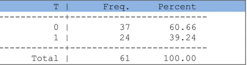
Table 3 illustrates the sample sizes of the regions with Z within ½ SD away from the cut-off

point (i.e. with values of Z between 60.70% and 89.30%).

Table 3 : Sample sizes of NUTS2 regions within 1/2 SD from cut-off of Z (60.70% <Z >89.30%)

T | Freq. Percent

---+---

0 | 37 60.66

1 | 24 39.24

---+---

Total | 61 100.00

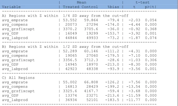
4.2 Descriptive statistics on the balance of the pre-intervention covariates

(X) between Obj.1 and non-Obj.1 regions

In order to draw comparisons between the PSM and the RDD results, it is useful to investigate

how the pre-intervention (1991-1994) characteristics of the Obj1. and non-Obj.1 regions are

balanced. This is done separately for the set of X

(control variables in terms of

pre-intervention growth) and of X

(control variables in terms of average pre-intervention levels)

and for three different groups of regions based on their values of the forcing variables “Z”:

14

a) regions with values of Z just above or the below the cut-off (i.e. within ¼ SD away

from the cut-off);

b) regions with values of Z +/- ½ SD from the cut-off;

c) regions with any values of Z (i.e. the whole sample of regions).

The figures reported in Table 4 shows that for the growth rate pre-intervention covariates, the

overall balance between the Obj.1 regions (treated) and the non-Obj.1 regions (control) does

not improve much by restricting the sample of NUTS2 to only the regions with similar values of

the “forcing variable” Z (sample A), as supposed to whole sample of regions (C). Such finding

is consistent with the hypothesis that the “forcing variable “(Z) that does not capture all the

relevant pre-intervention growth-trends controls that may represent risk-factors for selection

Table 4 : Pre-intervention differences in Xgrw between Obj.1 (treated) and non-Obj.1 regions (control)

| Mean | t-test

Variable | Treated Control %bias | t p>|t|

---+---+---

A) Regions with Z within 1/4 SD away from the cut-off

d_emprate |-1.3534 -1.3031 -3.2 | -0.08 0.935

d_compens |-.24538 1.8341 -86.7 | -2.21 0.037

d_grsfixcapt |-1.4274 -.83096 -15.5 | -0.39 0.696

d_GDP | 1.1565 1.5455 -28.8 | -0.74 0.469

d_labprod | 2.6028 2.9452 -22.1 | -0.56 0.579

---

B) Regions with Z within 1/2 SD away from the cut-off

d_emprate |-1.3187 -1.0414 -21.3 | -0.84 0.406

d_compens |-.40011 1.6557 -80.7 | -3.36 0.001

d_grsfixcapt |-2.7986 -.20104 -59.4 | -2.34 0.023

d_GDP | .52153 1.5145 -67.6 | -2.67 0.010

d_labprod | 1.9545 2.6179 -37.3 | -1.43 0.159

---

C) All Regions

d_emprate |-.90036 -1.0859 15.1 | 0.98 0.326

d_compens | 3.1352 1.24 35.9 | 2.86 0.005

d_grsfixcapt | -1.042 .02656 -21.7 | -1.39 0.166

d_GDP | 1.7761 1.0389 17.7 | 1.36 0.174

d_labprod | 2.7872 2.1785 14.0 | 1.08 0.279

---

For what is concerns instead the set of control variables in terms of average pre-intervention

levels (Table 6), the balance between the treated (Obj.1) and control (non-Obj.1) regions does

somehow improves by considering solely the NUTS2 areas with similar values of Z (sample A)

as supposed to the whole sample (C). ). Such finding is consistent with the hypothesis that the

“forcing variable “(Z) is somehow correlated solely with the pre-intervention average levels of

the control variables that may represent risk-factors for selection bias.

15

Table 5 : Pre-intervention differences in X

between Obj.1 (treated) and non-Obj.1 regions (control)

| Mean | t-test

Variable | Treated Control %bias | t p>|t|

---+---+---

A) Regions with Z within 1/4 SD away from the cut-off

avg_emprate | 53.552 59.864 -79.4 | -2.03 0.054

avg_compens | 20073 27294 -174.0 | -4.44 0.000

avg_grsfixcapt | 3370.2 3705.6 -36.0 | -0.92 0.368

avg_GDP | 16049 19299 -153.7 | -3.92 0.001

avg_labprod | 44844 49933 -73.2 | -1.87 0.074

---

B) Regions with Z within 1/2 SD away from the cut-off

avg_emprate | 52.289 60.146 -111.2 | -4.31 0.000

avg_compens | 19065 27060 -179.5 | -7.10 0.000

avg_grsfixcapt | 3356.5 3712.3 -28.6 | -1.03 0.306

avg_GDP | 14945 18970 -213.0 | -8.30 0.000

avg_labprod | 42923 48338 -93.9 | -3.56 0.001

---

C) All Regions

avg_emprate | 55.002 66.808 -126.2 | -7.56 0.000

avg_compens | 16813 28429 -199.2 | -13.54 0.000

avg_grsfixcapt | 3325.6 4167.7 -59.4 | -3.68 0.000

avg_GDP | 13374 23271 -213.6 | -11.59 0.000

avg_labprod | 36934 52101 -183.5 | -11.77 0.000

---

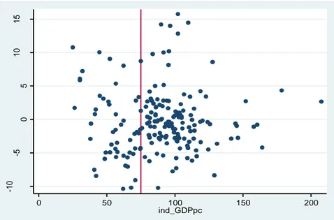
To further investigate how dominant is the “forcing variable” (Z) in controlling for some

pre-intervention regional covariates that may be linked with future regional growth, we plot each

value of Z against the corresponding value of each control variable, both in terms of

pre-intervention growth-trends (Figures 1-5) and in terms of pre-pre-intervention average levels

(figures 6-10). In Figures 1-10, the cut-off point of the “forcing variable” Z (1988-1990

per-cpaita GDP as a % of EU mean) is indicated with a vertical red line.

16

Figure 1 : Pre-intervention annual % change in the employment rate (1=p.p.) plotted against values of Z

(per-capita GDP in 1988-90 in terms of % of EU mean)

Figure 2 : Pre-intervention annual % growth in GDP per-capita (1=p.p.) plotted against values of Z

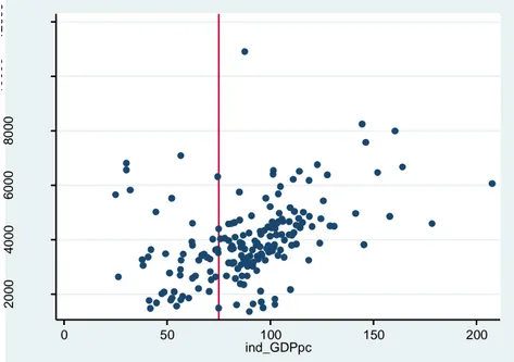
(per-capita GDP level in 1988-90 in terms of % of EU mean)

-6 -4 -2 0 2 a ve ra g e a n n u a l % ch a n g e o f e m p lo yme n t ra te w it h re g a rd t o t p o p u la ti o n (1 = 1 p e r 0 50 100 150 200 ind_GDPpc -5 0 5 10 15 20 a ve ra g e a n n u a l p e rce n ta g e ch a n g e o f th e p e r ca p it a g d p -co mp i n te re st f o rmu la 1 = 0 50 100 150 200 ind_GDPpc

17

Figure 3 : Pre-intervention annual % change in worker compensation (1=p.p.) plotted against values of Z

(per-capita GDP in 1988-90 in terms of % of EU mean)

Figure 4 : Pre-intervention annual % growth in per-capita fixed capital formation (1=p.p.) plotted against

values of Z (per-capita GDP level in 1988-90 in terms of % of EU mean

-1 0 0 10 20 a ve ra g e a n n u a l p e rce n ta g e ch a n g e o f th e p e r ca p it a e mp lo yme n t co mp e n sa ti o n (1 = 1 0 50 100 150 200 ind_GDPpc -1 0 -5 0 5 10 15 a ve ra g e a n n u a l p e rce n ta g e ch a n g e o f th e p e r ca p ita f ixe d ca p ita l f o rma tio n -co mp 0 50 100 150 200 ind_GDPpc

18

Figure 5 : Pre-intervention annual % growth (1=1 p.p.) in labour productivity (GDP per-worker) plotted

against values of Z (per-capita GDP level in 1988-90 in terms of % of EU mean)

The plotted charts of Figures 1-5 illustrates well a lack of a strong correlation between the

values of the “forcing variable” Z and the pre-intervention growth-rate of the control variables

used in the analysis. Such lack of correlation does not ensure, in the presence of small

samples, that an adequate balancing between the pre-intervention growth-trends is achieved

between the Obj.1 (treated) and non-obj1 (non-treated) regions that have values of the

“forcing variable” Z close to the cut-off point.

The plotted charts of Figures 6-10, instead, depict a fairly evident correlation between the

“forcing variable” Z and the average pre-intervention values of the control variables. Such

correlation has two important implications for the analysis:

a) The regions with balanced pre-intervention levels of the control variables across the

treatment and comparison group, tend to be those with values of Z in the

neighbourhood of the cut-off point;

b) The overall number of regions on the common support (i.e. with balanced

pre-intervention characteristics) is drastically reduced when the control variables are

operationalized also in terms of levels as supposed to solely in terms of growth trends.

-5 0 5 10 15 20 a ve ra g e a n n u a l p e rce n ta g e ch a n g e o f G D P p e r w o rke r -co mp in te re st f o rmu la 1 = 1 p 0 50 100 150 200 ind_GDPpc

19

Figure 6 : Pre-intervention average level of employment rate (1=1%) plotted against values of Z

(per-capita GDP in 1988-90 in terms of % of EU mean)

Figure 7 : Pre-intervention average level of GDP per-capita (1=EUR) plotted against values of Z (per-capita

GDP level in 1988-90 in terms of % of EU mean)

40 60 80 1 0 0 1 2 0 a ve ra g e a n n u a l e mp lo yme n t ra te (1 = 1 % ) 0 50 100 150 200 ind_GDPpc 1 0 0 0 0 2 0 0 0 0 3 0 0 0 0 4 0 0 0 0 5 0 0 0 0 6 0 0 0 0 a ve ra g e a n n u a l le ve l o f th e p e r ca p it a g d p 1 = 1 EU R p e r re si d e n t 0 50 100 150 200 ind_GDPpc

20

Figure 8 : Pre-intervention average level of worker compensation (1=EUR) plotted against values of Z

(per-capita GDP in 1988-90 in terms of % of EU mean)

Figure 9 : Pre-intervention average level of per-capita fixed capital formation (1=EUR) plotted against

values of Z (per-capita GDP level in 1988-90 in terms of % of EU mean)

1 0 0 0 0 2 0 0 0 0 3 0 0 0 0 4 0 0 0 0 5 0 0 0 0 a ve ra g e a n n u a l p e r ca p it a e mp lo yme n t co mp e n s a ti o n 1 = 1 EU R p e r w o rke r) 0 50 100 150 200 ind_GDPpc 2 0 0 0 4 0 0 0 6 0 0 0 8 0 0 0 1 0 0 0 0 1 2 0 0 0 a ve ra g e a n n u a l le ve l o f th e p e r ca p it a f ixe d ca p it a l fo rma ti o n 1 = 1 EU R 0 50 100 150 200 ind_GDPpc

21

Figure 10 : Pre-intervention average level of labour productivity (GDP per-worker, 1=1 EUR) plotted

against values of Z (per-capita GDP level in 1988-90 in terms of % of EU mean)

2 0 0 0 0 4 0 0 0 0 6 0 0 0 0 8 0 0 0 0 1 0 0 0 0 0 a ve ra g e a n n u a l le ve l o f th e G D P p e r w o rke r 1 = 1 EU R p e r w o rke r 0 50 100 150 200 ind_GDPpc

22

5.

Methods: Propensity Score Matching estimation

The estimates of the impact of the additional EUF related to Obj.1 eligibility on the 1995-2006

average per-capita GDP growth have been obtained from the following Propensity Score

Matching (PSM) models:

•

Radius Matching;

•

Nearest Available Caliper Matching;

•

Kernel Matching.

5.1 Radius Matching estimators

Radius matching estimators were implemented in the analysis with different values of the

tolerance radius (



) and the following different specifications of the control variables:

•

Growth-rate trends (X

) in terms of pre-intervention: employment rate (emplrate);

worker compensation (wrk_compens), per–capita GDP (GDP), gross fixed capital formation

(gross_fxd_cap_form) and labour productivity (in terms of GDP per-worker: lab_prod);

•

Three growth-rate trends and three average-level controls (wrk_compens, GDP,

gross_fxd_cap_form);

•

A full set of controls (X

X

) in terms of pre-intervention both growth-trends and levels

(emplrate; wrk_compens; GDP; gross_fxd_cap_form; lab_prod).

Formally the estimation procedure entailed the following steps:

a) Estimation of three different probit specifications:

P(T=1) =



(X

)

(1)

or

P(T=1) =



(X

)

(2)

or

P(T=1) =



(X

, X

)

(3)

Where:

T=1 receiving the additional EU fund aid intensity related to the Obj.1 area

designation;

X

= set of pre-intervention (1991-1994) control variables in terms average

annual growth-rate trends of: employment rate (emplrate); worker

compensation (wrk_compens), per–capita GDP (GDP), gross fixed capital

formation (gross_fxd_cap_form) and labour productivity (in terms of GDP

per-worker: lab_prod);

X

= set of six pre-intervention (1991-1994) control variables composed by

three average annual growth-rate trends and three average annual levels of:

worker compensation (wrk_compens), per–capita GDP (GDP), gross fixed capital

formation (gross_fxd_cap_form);

23

X

= set of pre-intervention (1991-1994) control variables in terms average

annual levels of: employment rate (emplrate); worker compensation

(wrk_compens), per–capita GDP (GDP), gross fixed capital formation

(gross_fxd_cap_form) and labour productivity (in terms of GDP per-worker:

lab_prod).

b) The predicted probabilities T

₌

_

_(X

_

_{) from the three probit specifications (1-3)}

represents three sets of Propensity Scores (PS) alternatively used for matching each

single Obj.1 region with the non-Obj.1 regions sharing the most similar

pre-intervention (1991-1994) characteristics. Such matching procedure is implemented

with a radius of tolerance (



) that represents the maximum distance (in absolute

value) between the PS of the Obj,1 regions (T=1) and those of the non-Obj.1

regions (T=0) that are matched together. The radius (



) that were used in the

analysis were alternatively: 0.005; 0.01; 0.05; 0.10; 0.15

_.

c) Once each Obj.1 region is matched with the group of non-Obj1 regions that shares

similar pre-intervention characteristics in terms of either X

X

or both X

and

X

, the impact estimates in terms of Average Treatment Effects on the Treated

(ATT) parameters



are retrieved as:



= E [Y

_{| T=1, PS]- E [Y}

_{| T=0, PS]}

₍₄₎

5.2 Nearest Available Caliper Matching

The Nearest Available Caliper Matching estimators were implemented in the analysis with

different values of the caliper (



) and the same three different sets of control variables used for

the Radius Matching estimation: (X

), (X

) and (X

, X

). Formally the estimation

procedure entailed the following steps:

a) Estimation of the three different probit specifications (1), (2), (3).

b) The predicted probabilities T

₌

_

_(X

_

_{) from the three probit specifications (1-3)}

represents three sets of Propensity Scores (PS) alternatively used for matching each

single Obj.1 region with the single non-Obj.1 region that shares the most similar

pre-intervention (1991-1994) characteristics. Such matching procedure is

implemented with a caliper (



) that represents the maximum distance (in absolute

value) between the PS of the Obj.1 region (T=1) and the matched non-Obj.1 region

(T=0). Obj.1 regions that have a closest non-Obj.1 region with a PS outside the

caliper of tolerance (



) are discharged from the analysis. Similarly as for the radius

matching, the caliper(



) that were used in the analysis were alternatively: 0.005;

0.01; 0.05; 0.10; 0.15

_.

c) Once each Obj.1 region is matched with the non-Obj1 region that shares the most

similar pre-intervention characteristics in terms of either X

X

or both X

and

4 _{The results presented in this report will be drown from the specifications of the radius () that ensure}

the best overall balancing of the pre-intervention control variables, while the complete sets of results will be presented in the Appendix.

5 _{The results presented in this report will be drown from the specifications of the caliper () that ensure}

the best overall balancing of the pre-intervention control variables, while the complete sets of results will be presented in the Appendix.

24

X

, the impact estimates in terms of Average Treatment Effects on the Treated

(ATT) parameters



are retrieved as in (4).

5.3 Kernel Matching

The Kernel Matching estimators were implemented in the analysis with the following different

smoothing functions:

•

Gaussian, with different bandwidth (the STATA default 0.06, 0.1 and 0.15

_);

•

Biweight;

•

Epanechnikov.

The set of control variables used for the estimation are the same (X

), (X

) and (X

, X

)

used for radius and nearest neighborhood matching. More in detail, the estimation procedure

entailed the following steps:

a) Estimation of the three different probit specifications (1), (2), (3).

b) The predicted probabilities T

₌

_

_(X

_

_{) from the three probit specifications (1-3)}

represents three sets of Propensity Scores (PS) alternatively used for the Kernel

matching procedures based on the different smoothing functions.

c) The outcome (Y

_{) of each Obj.1 region is compared with a weighted average of the}

outcomes (Y

_{) of each non-Obj.1 region with the weights of such average being}

inversely proportional to the distance between the PSs. One of the three different

smoothing functions alternatively used in the analysis sets the pace of the decline in

the importance of each non-Obj.1 area in contributing to the comparison average

(Y

_{) as the PS of the non-Obj.1 area gets more distant from that of the Obj.1 area.}

5.4 PS estimation and common support

The goal of the Propensity Score Matching (PSM) procedures used in the analysis is to produce

impact estimates based on comparisons between Obj.1 regions and regions with similar

1991-1994 growth potentials that were not designated as Obj.1 areas. No matter which PSM

procedure is used, the potential for obtaining good internal and external validity for the

analysis crucially relies on the whether or not and actual adequate balancing of the

pre-intervention control variables exists between the treatment (Obj.1 regions) and the comparison

group (non-Obj1 regions). The existence of such balancing is ensured in the presence of

adequate “common support” in the estimated Propensity Scores (PS, which can be though as a

variable which summarizes the relevant pre-intervention confounding factors). In the following

Figures 11-13 we depict the boxplots of the PS distributions for the treatment and the

comparison group. An adequate balancing of the 1991-1994 control variables would produce a

large overlapping between the PS distributions of the Obj.1 and non-Obj.1 regions (i.e. an

extensive “common support” is detected).

6 _{The results in this report will be based on the bandwidth that ensure the best overall balancing of the}

25

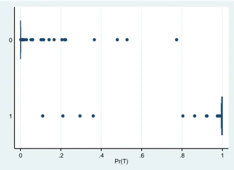
Figure 11 : Boxplots of the PS distributions based on Xgrw (Growth-trends controls) [All Regions]

T=0 (above): comparison group

T=1 (below): treatment group

0 .2 .4 .6 .8

Pr(T) 1

26

Figure 12 : Boxplots of the PS distributions based on three Xgrw (Growth-trend controls) and three Xlev

(Average-level controls). [All Regions]

T=0 (above): comparison group

T=1 (below): treatment group

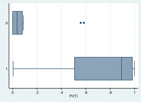
Figure 13 : Boxplots of the PS distributions based on all Xgrw (Growth-trend controls) and Xlev

(Average-level controls). [All Regions]

T=0 (above): comparison group

T=1 (below): treatment group

0 .2 .4 .6 .8 1 Pr(T) 1 0 0 .2 .4 .6 .8 1 Pr(T) 1 0

27

As shown in Figures 11-13, the “common support” of the PS distributions for the treated and

the comparison group is much larger when the analysis is implemented based on the

growth-trend control variables. This is not surprising as the forcing variable Z which determined the

treatment assignment captured the average per-capita GDP in the years 1988-1990. For this

reason, the distribution of the average pre-intervention levels of the control variables is much

different between the treatment and the comparison group than the distribution of the

pre-intervention growth-trends.

As a consequence PSM estimators that will include also control variables in terms of average

pre-intervention levels will likely suffer from low common support, and weak statistical

efficiency (low significance) and external validity. This is due to the small sample of regions for

which the full set of growth-rates and average-levels control variables are balanced between

the treatment and the comparison group.

When the average-level of the control variables are used in the analysis, the unbalance

between the treatment and the comparison group is not much mitigated even by restricting the

focus solely on the regions close to the cut-off of the forcing variable Z (Figures 14-16). Thus,

applying such restricted focus on the regions in the neighbourhood of the cut-off would yield

the same (if not greater) weak statistical efficiency and external validity as in the case of PSM

estimators implemented on the common support.

Figure 14 : Boxplots of the PS distributions based on Xgrw (Growth-trends controls). [Regions close to the

cut-off of eligibility: Z within 1/4 SD away from the cut-off]

T=0 (above): comparison group

T=1 (below): treatment group

0 .2 .4 .6 .8

Pr(T) 1

28

Figure 15 : Boxplots of the PS distributions based on three Xgrw (Growth-trend controls) and three Xlev

(Average-level controls). [Regions close to the cut-off of eligibility: Z within 1/4 SD away from the cut-off]

T=0 (above): comparison group

T=1 (below): treatment group

Figure 16 : Boxplots of the PS distributions based on all Xgrw (Growth-trend controls) and Xlev

(Average-level controls)

The set of boxplot figures reported above indicates the presence of a trade-off for the analysis:

controlling for pre-intervention trends ensures higher efficiency, external validity and balancing

0 .2 .4 .6 .8 1 Pr(T) 1 0 0 .2 .4 .6 .8 1 Pr(T) 1 0

29

of the growth-rate controls. If also average-levels of the region pre-intervention characteristics

are to be controlled for, the available data do allow impact identification only for a very small

number of regions on the common support (with low statistical efficiency and external validity).

30

6.

Summary of the results (Task 1)

The main results from the analysis are reported in Tables 6-8, which contain the impact

estimates of the PSM specifications that offer the best overall balancing of the pre-intervention

covariates within each of the three different types of matching procedures used in the analysis:

radius, nearest available with caliper and kernel. The complete set of results for all the

estimated specifications are contained in the Technical Appendix.

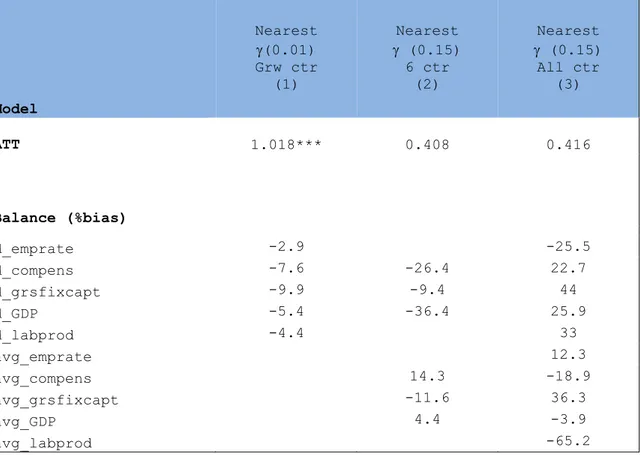
Table 6 : Results from the PS Radius Matching estimators (preferred specifications with the best

balancing of the control variables)

Radius

(0.01)

Grw ctr

(1)

Radius

(0.01)

6 ctr

(2)

Radius

(0.15)

All ctr

(3)

ATT

0.829***

0.528

0.368

Balance (%bias)

d_emprate

-5.5

-11.1

d_compens

-5.4

-20

20.5

d_grsfixcapt

-12.8

-3.3

14.4

d_GDP

-10

-37

8.1

d_labprod

-8.1

11.7

avg_emprate

8.4

avg_compens

12.2

-9.2

avg_grsfixcapt

-20.2

55.2

avg_GDP

-10.6

-10.3

avg_labprod

-31.7

The results from the PS radius matching estimator reported in Table 6 indicate that the

additional intensity of the EUF associated with the Obj.1 eligibility

_{generated an average of}

+0.82 percentage points (p.p.) in the yearly growth rate of the per-capita GDP during the

1995-2006 period. Such additional growth-rate gain is estimated compared to the

counterfactual yearly growth rate that would have occurred in the absence of the additional

Obj.1 intensity of the EUF. The +0.82 (p.p.) estimated impact is obtained by estimating the

counterfactual trend through the yearly GDP data from the non-Obj.1 regions that shared

similar pre-intervention (1991-1994) growth trends (column 1 of Table 6) of the Obj.1 regions

in terms of: employment rate (emplrate); worker compensation (wrk_compens), per–capita

7_{As mentioned before, such additional intensity corresponds to a per-capita overall value of EU funds}

greater than 1960 Euro. Further details on the distribution of the per-capita EU funds 1995-2006 expenditures between Obj.1 and non-Obj.1 regions can be found in Pellegrini et al. 2013.

31

GDP (GDP), gross fixed capital formation (gross_fxd_cap_form) and labour productivity (in

terms of GDP per-worker: lab_prod).

When the set of control variables used in the analysis includes instead both the growth trends

and the average pre-intervention levels of three control varaibles [Column 2 of Table 6: worker

compensation (wrk_compens), per–capita GDP (GDP), gross fixed capital formation

(gross_fxd_cap_form)], the estimated impact (+0.53 p.p.) fails to reach statistical significance.

As discussed in the previous sections, this is due to the smaller common support between the

treatment and the comparison group that is encountered when also the average

pre-intervention levels of the control variables are included in the analysis. The same small

common support issues plagues also the estimates from the PS specification that includes the

full set of growth-trends and average pre-intervention levels for all the control variables

considered in the analysis [column 3 of Table 6: employment rate (emplrate); worker

compensation (wrk_compens), per–capita GDP (GDP), gross fixed capital formation

(gross_fxd_cap_form) and labour productivity (in terms of GDP per-worker: lab_prod)].

The results from the PS nearest available caliper matching (Table 7) and the Kernel matching

(Table 8) follows a similar pattern to those from the PS radius matching. The specification (1)

that controls for the pre-intervention growth-rate trends yields statistically significant impact

estimates with magnitude close to the that of the radius matching: +1.01 p.p. for the nearest

available matching (Table 7, column 1); + 0.90 p.p. for the Kernel matching (Gaussian

smoothing function). For both the nearest available and the kernel matching estimators,

similarly to the radius matching, the specifications that controls also for the pre-intervention

average levels (in addition to the pre-intervention growth trends) yield impact estimates with

no statistical significance: +0.40 and +0,41 p.p. for the nearest available matching estimator

(Table 7, columns 2 and 3, respectively); +0.53 and +0.34 p.p. for the Gaussian Kernel

matching estimator (Table 8, columns 2 and 3 respectively).

32

Table 7 : Results from the PS Nearest Available estimators with Caliper (preferred specifications)

Model

Nearest



(0.01)

Grw ctr

(1)

Nearest



(0.15)

6 ctr

(2)

Nearest



(0.15)

All ctr

(3)

ATT

1.018***

0.408

0.416

Balance (%bias)

d_emprate

-2.9

-25.5

d_compens

-7.6

-26.4

22.7

d_grsfixcapt

-9.9

-9.4

44

d_GDP

-5.4

-36.4

25.9

d_labprod

-4.4

33

avg_emprate

12.3

avg_compens

14.3

-18.9

avg_grsfixcapt

-11.6

36.3

avg_GDP

4.4

-3.9

avg_labprod

-65.2

33

Table 8 : Results from the PS Kernel Matching estimators, Gaussian with bandwidth (preferred

specifications)

Model

Kernel Gaus



(0.01)

Grw ctr

(1)

Kernel Gaus



(0.06)

6 ctr

(2)

Kernel Gaus



(0.15)

All ctr

(3)

ATT

0.901***

0.528

0.339

Balance (%bias)

d_emprate

-3.6

-18

d_compens

-6.2

-18.9

21.9

d_grsfixcapt

-10.2

-1.1

20.3

d_GDP

-9.7

-37.7

10.8

d_labprod

-8.3

16.3

avg_emprate

10.5

avg_compens

13.9

-12.5

avg_grsfixcapt

-19.3

49

avg_GDP

-10.2

-12.6

avg_labprod

-40.3

34

7.

Concluding remarks (Task 1)

The main goal of Task1 was to draw a comparison between RDD and PSM in estimating the

impact of EUF on regional growth. This is done both through reviewing and comparing some

theoretical properties of the two types of estimators and by replicating with PSM the

dichotomous-treatment RDD analysis implemented in the literature (Pellegrini et al. 2013). The

main findings of this study can be summarized as follows:

•

RDD and PSM are both viable ways to implement regional-level CIEs of the EUF, however,

because no true self-selection into applying occurred: RDD does not have the advantage of

better controlling for unobservable regional characteristics;

•

In order to decide which approach to use: it’s crucial to assess how dominant is the

forcing variable as a confounding factor that captures all major risk-factors for selection

bias and how large is sample of regions near the cut-off point of the forcing variable. If the

forcing variable is non-dominant and the sample size is small, RDD may fail to ensure

proper balancing of the relevant control variables (in the same way as randomized

experiments may fail to ensure proper balancing of all relevant confounding factors with

small samples). In such circumstance, statistical matching between regions above and

below the cut-off point of the forcing variable can be seen as conceptually similar to a

block randomization design (with regard to the relevant control variables) to ensure proper

balancing in the presence of small samples of regions;

•

If little common support is found for certain controls: both the external validity and the

statistical efficiency of the estimates will suffer. The ultimate decisions on the types and

number of control variables to be used in the analysis should be based on specific

knowledge about factors that have been linked to future regional growth;

•

The results from the present PSM analyses show that the EUF, in the 1995-2006 period,

spurred additional growth in the amount of 0.8-1 p.p. These results are estimated under

the assumption that important confounding factors to be controlled for are the

pre-intervention growth-rate trends of the control variables;

•

If instead also the pre-intervention average levels of the control variables are included in

the Propensity Score estimation, the impact of the EUF on the regional GDP growth is

somehow lower (0.3-0.5 pp) and the impact estimates fail to reach statistical significance

because of a very small common support between the treatment and the comparison

group.