S
CUOLAN
ORMALES
UPERIOREP
H.D
.
THESIS
IN
BIOPHYSICAL SCIENCES
Capturing molecular behavior in
dynamic subcellular nanostructures
Filippo Begarani
A
DVISORProf. Francesco Cardarelli
Foreword
This Thesis is the result of my research activity at NEST laboratory of Scuola Normale Superiore in Pisa: I began my PhD program studies in 2014, supported by Professor Francesco Cardarelli and his group where I found a stimulating and energetic environment loaded with profound ambition and deep scientific know-how; fundamental conditions necessary to carry out this PhD program in Biophysical Science.
List of publications
Begarani, F., D'Autilia, F., Signore, G., Del Grosso, A., Cecchini, M., Gratton, E., ... & Cardarelli, F. (2019). Capturing Metabolism-Dependent Solvent Dynamics in the Lumen of a Trafficking Lysosome. ACS nano 13, 2,
1670-1682
Begarani, F., Cassano, D., Margheritis, E., Marotta, R., Cardarelli, F., & Voliani, V. (2018). Silica-Based Nanoparticles for Protein Encapsulation and Delivery. Nanomaterials, 8(11), 886.
In preparation: Begarani, F., D'Autilia, F., Del Grosso, A., Cardarelli, F.
Investigating the dynamic behavior of molecular species in subcellular nanostructures by time-tunable raster-image correlation spectroscopy.
Table of Contents
Foreword ... 1 1. Introduction ... 5 1.1 Molecular information at the subcellular level in a non-natural environment ... 6
1.1.1 The biochemistry of intracellular structures/compartments studied in vitro ...7 1.1.2 The ultrastructure of subcellular structures/compartments studied at the wavenumber of electrons ...9 1.1.3 Studying subcellular structures/compartments by means of nanoscopic probes: Atomic Force Microscopy (AFM). ...11
1.2 “Chemical imaging” at the subcellular level: what perspectives? ... 12
1.2.1 Fourier Transform Infrared (FTIR) imaging ...12
1.3 Molecular information at the subcellular level from fluorescence-based optical microscopy ... 14
1.3.1 Localization-based methods: accuracy is a time-consuming task ...15 1.3.2 Structured illumination microscopy (SIM) ...19 1.3.3 Stimulated emission depletion microscopy (STED) ...20
1.4 Fluorescence Correlation Spectroscopy: a powerful tool to boost the spatiotemporal resolution of optical microscopy methods ... 23 2. Time-tunable Raster Image Correlation Spectroscopy to capture molecular diffusion in dynamic subcellular nanostructures ... 29
Table of Contents
2.1 Time-tunable RICS on dynamic subcellular nanosystems... 29
2.1.1 RICS analysis ...30
2.1.2 STICS analysis ...31
2.1.3 Time-tunable RICS validation on dynamic nanosystems in vitro ...33
2.1.4 Time-tunable RICS validation in biological samples ...37
2.2 Concluding remarks ... 42
3. Bringing RICS on the trajectory of single subcellular nanostructures by feedback-based 3D orbital tracking ... 45
3.1 From many organelles to a single organelle: the feedback-based 3D Orbital Tracking principle and setup ... 47
3.1.1 Circular-RICS analysis on the orbit: microseconds along the orbit, milliseconds between orbits ...48
3.2 ACDAN stability as a fluorescent marker of the lysosomal lumen ... 49
3.3 Feedback-based 3D Orbital tracking and RICS on single lysosomes ... 54
3.4 Concluding remarks ... 60
4. Capturing metabolism-dependent solvent polarity fluctuations in the lumen of a trafficking lysosome in physiology and disease ... 63
4.1 The Twitcher model and preliminary time-tunable RICS analysis ... 65
4.2 Circular-RICS on ACDAN GP carpets ... 67
4.3 ACDAN GP fluctuations and metabolic activity ... 76
4.4 ACDAN GP fluctuations in a cellular model of LSD ... 79
4.5 ACDAN-GP data interpretation... 87
4.5 Concluding remarks ... 91
Table of Contents
Appendices ... 99
A. Experimental setup for feedback-based orbital tracking and RICS ... 101
A.1 Confocal microscopy imaging ...101
A.2 Live-cell confocal microscopy imaging and co-localization ...102
A.3 Orbital tracking setup and experiments ...103
A.4 Software used for FCS analysis ...104
A.5 FCS analysis of ACDAN GP ...104
A.6 Acquisition of ACDAN Fluorescence Spectrum and Evaluation of GP ...105
A.7 Calibration of the hydrodynamic radius of QDs ...106
A.8 Statistical Analysis ...106
B. Sample preparation ... 107
B.1 Cell culture and treatments ...107
B.2 Liposomes containing QDs 545: partially immobilized in Agarose gel ...108
B.3 Preparation of fluorophore solutions ...109
C. Protein encapsulation and delivery through silica-based nanoparticles ... 111
C.1 A brief introduction to protein delivery... 112
C.2 SynThesis and characterization of the nanoparticles ... 114
C.3 Cellular uptake and final fate of nanoparticles ... 118
C.4 Particle stability in acidic conditions... 120
C.5 Concluding remarks ... 121
Table of Contents
List of Figures... 139 List of Tables ... 143
Introduction 1
Foreword
It is no coincidence that modern Biophysics is commonly thought to have been born with the words pronounced by Erwin Schrödinger during his lectures held in 1943 at Trinity College in Dublin and collected in the book “What is Life? The Physical Aspect of the Living Cell”1. Wondering about
the complexity of life, Schrödinger admirably defines what will be, from then on, the main concern of an experimental biophysicist, that is, in his words:
"how can the (molecular) events in space and time which take place within
the spatial boundary of a living organism be accounted for by physics and chemistry?" Capturing the intrinsic spatial and temporal dimension of life regulation is a challenge that biophysicists have been increasingly embracing, building on nearly a century of studies at a variety of length scales. Over the last decades, the focus of biophysics progressively shifted from the macroscale to the nanoscale. Here, main actors are the molecules. To successfully address the intrinsic spatial and temporal scales of molecular behavior, two crucial requisites are needed: (1) nanometer spatial resolution (to tackle the spatial scale of molecules), (2) micro-to-millisecond temporal resolution (to probe the time scale that is relevant for molecular processes). In this context, optical microscopy is a valuable methodological approach. First, at wave numbers of visible light, and using fluorescence as readout, both the spatial and temporal scales can be investigated directly in living matter. In addition, the recently-developed super-resolution technologies2 circumvented
the remaining limit imposed by diffraction and pushed biophysical investigations to the true nanoscale.
2 Introduction
In spite of these achievements, life regulation is destined to remain elusive in a natural condition of living matter, that of subcellular, membrane-enclosed nanosystems: transport vesicles, organelles, or entire subcellular protrusions. Here, the leading molecular actors are part of a reference nanosystem that is endlessly changing position in space and time in the complex 3D cellular environment. This peculiar condition imposes that a third requisite be concomitantly met in the same experiment, that is: (3) large volume sampling to localize the nanosystem. Unfortunately, however, volume sampling and temporal resolution are mutually-dependent parameters, i.e. the larger the volume to probe, the lower the temporal resolution achievable.
The overriding goal of my PhD Thesis is to grab the physics of life regulation at the level of nanoscopic, dynamic subcellular systems. By bringing state-of-the-art biophysical tools along the 3D-trajectory of the target system, unprecedented spatiotemporal resolution will be achieved to (i) enlighten the hitherto elusive realm of molecular processes occurring in the new reference system, and (ii) plan breakthrough experiments to interrogate living-matter physiopathology at the subcellular scale.
This Aim will be pursued by two main methodological and technological implementations at the subcellular scale, namely: (i) time-tunable Raster Image Correlation Spectroscopy (RICS) to analyze the average dynamic behavior (i.e. diffusion) of molecules within a population of subcellular nanosystems (i.e. organelles or compartments) and (ii) the combination of fast RICS with feedback-based 3D orbital imaging&tracking of a single intracellular nanosystem per time in order to maximize the temporal resolution achievable to look at molecular behavior.
In time-tunable RICS, a confocal microscope is used to capture standard images of the sample with a raster-scanning laser beam. Time-tunable RICS is achieved by acquiring consecutive stacks of images using different pixel
Introduction 3
dwell times. Each scan speed is used as a filter to select the characteristic temporal scale of molecular behaviour that significantly contributes to the measured correlation function. This approach covers a hitherto unexplored dynamic range, as determined by available pixel dwell times, from 0.5 μs to several milliseconds.
On the contrary, by feedback-based 3D orbital imaging&tracking, the light-beam is sent in a periodic orbit around the nanostructure of interest. The recorded signal (e.g. fluorescence or scattered light) is used as feedback to localize the nanostructure position with unprecedented spatiotemporal resolution. The acquired, privileged observation point will be used to push single-molecule studies to an entirely new level, exploiting the analytical tools mentioned above (i.e. RICS analysis).
For the sake of clearness, results are organized as described in the following: − In Chapter 1, a review of the more common imaging-based techniques developed for quantitative molecular analysis at the subcellular level is reported. In this Chapter, each technique is presented highlighting advantages and drawbacks, with a particular emphasis on the peculiar spatial and temporal resolution, i.e. on the ability of each technique to grab the dynamic behavior of molecules at the subcellular level.
− In Chapter 2, time-tunable RICS is introduced, with a particular focus on its application to the study of dynamic molecular processes hosted within subcellular nanosystems which are dynamic as well. The diffusion of a variety of fluorescent molecules is measured on different paradigmatic subcellular structures or organelles (e.g. lysosomes, mitochondria, secretory granules, etc.) either in their lumen or on their membrane.
− In Chapter 3, RICS analysis is combined with feedback-based 3D orbital imaging&tracking. The Lysosome is selected as the main case-study here and the dynamics of different molecules either within lysosome lumen or on its membrane are measured to validate the
4 Introduction
approach. The results obtained serve as a solid reference to introduce the subject of the next Chapter.
− In Chapter 4, RICS analysis along the orbit is used to unveil quantitatively the spatiotemporal fluctuations of the solvent contained in the lumen of lysosomes trafficking within living cells. Once again, lysosomes are chosen as a paradigmatic example of biomedical interest: different physiological and pathological conditions are tested.
− In Chapter 5, in conclusion of my work, possible implementations to improve the performances of the presented approaches are discussed, together with potential future applications in biophysics and related fields.
Chapter
1
___________________________________________________________________
1.
Introduction
Cells contain distinct dynamic, membrane-enclosed sub-compartments with sizes spanning from tens of nanometers (e.g. synaptic vesicles, caveolae, clathrin-coated pits) to hundreds of nanometers (e.g. endosomes, lysosomes, mitochondria, secretory granules), to several microns (e.g. Golgi apparatus, Endoplasmic Reticulum, nucleus). In addition, each of these mentioned cellular compartments is designed to concentrate specific sets of components and functions3. This aspect of organization determines, in turn, a
discontinuous and heterogeneous landscape of molecular composition, molecular functions and physicochemical properties within the cell.4. These
properties, in turn, play an active major role in the regulation of the biochemical processes representative of each specific district. To study the heterogeneity of subcellular organization, the choice of the most suitable technique becomes crucial. Being able to assess both chemical, biological and physical properties within the correct spatial and temporal scales is
6 State of the Art
everything. At present, there are no techniques that makes all these aspects available at once, but few attempts to go towards that direction.
In particular, our ability to study molecular behavior at this level is severely hindered by the restless, rapid movement of the entire reference system in the 3D cellular environment. State-of-the-art optical microscopy tools for delivering subcellular information at molecular resolution fail to subtract the 3D evolution of the entire system while preserving the spatiotemporal resolution required to probe dynamic molecular events.
1.1 Molecular information at the subcellular level in a non-natural
environment
The eukaryotic cell is characterized by a complex and well-organized mixture of biomolecules showing the most diverse functions and characteristics. Proteins, lipids, nuclei acids and other biomolecules get organized inside cells in an efficient and practical fashion to give birth to nuclei, cytoplasm, plasma membranes and a plethora of membrane-enclosed intracellular organelles to execute the most diverse functions.3 The survival and function of every living
organism and in particular of cell is thus strictly related to its internal organization, where multiple structures execute all the necessary tasks for cell homeostasis. It is for this reason that the term ‘organelle’ today is used to described specific intracellular environment where highly specialized functions take place2.
These function-specific environments, whether they are found as membrane-enclosed or membrane-less organelles, comprise large protein complexes such as the signalosomes or protein-RNA complexes such as the ribosomes but also membrane-bound specific structures such as the mitochondria, the lysosomes, the exosomes, the Golgi apparatus and so forth2,3,5. In order to
study these function-specific subcellular environments, many techniques and tools have been developed in the course of the human history, but, the
State of the Art 7
discoveries made in the last 100 years, with the advent of the transistor-based electronics, computer science, nanotechnology and Molecular Quantum Mechanics, along with their first experimental applications in the analysis of living organisms, paved the way to the development of a series of techniques that today represent the basis of ì Biophysics as a science.
1.1.1 The biochemistry of intracellular structures/compartments studied
in vitro
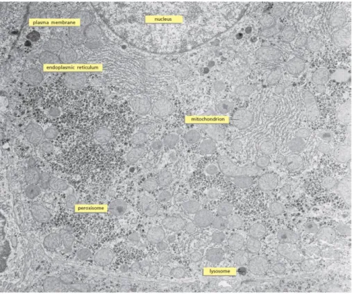
Subcellular analysis was ideally born in 1682 thanks to the pioneer work of the microscopist Antoine Van Leeuwenhoek who first discovered the nucleus in cod and salmon red blood cells (Fig. 1.1). Mitochondria and Golgi apparatus were instead first described respectively in 1850’s by Rudolph Albert von Kolliker and in 1890’s by Camillo Golgi. Their observations were only possible thanks to the employment of the first, rudimental, optical microscopes. As a matter of fact, with the advent of transmission electron microscopy, in the 1940s and 1950s, the study of intracellular organelles began, and structures such as the endoplasmic reticulum (ER) and peroxisomes were discovered. In the same period, electron microscopy was accompanied by biochemical studies of the cell and its components. Cellular fractionation by centrifugation allowed, in this sense, for the discovery of other subcellular organelles such as the lysosomes in 1955 by Christian de Duve2. The importance of analysing these structures in terms of their
molecular content was first addressed by O’Farrell and colleagues in 1977 via gel electrophoresis6. In this context, organelle proteomics helped to unveil the
content of many subcellular structures7–11. A significant boost of this activity
was imposed by the advent of mass-spectrometry-based approaches. The first demonstrations of mass spectrometry used for subcellular analysis dates back to the years 1984-85 when Richard W. Gross published his results on mitochondria and plasma membrane12,13. Since then, mass spectrometry
8 State of the Art
techniques such as Matrix-assisted laser desorption/ionization (MALDI) and Desorption electrospray ionization (DESI) have evolved to address subcellular contents.
However, all these techniques imply either the isolation of the organelles from their original environment (i.e., the cell) or the disruption of the structure itself. For instance, all the analytical tools created for organelle proteomics necessarily require the isolation of the organelles from the cells, thus altering their natural surrounding environment and consequently the complex dynamic behaviours they would assume within. Mass spectroscopy instead, works by extracting ionized atoms from the sample surface, thus destroying the sample as it is being analysed. It is for these reasons that these disruptive approaches will not be part of in this dissertation.
State of the Art 9
1.1.2 The ultrastructure of subcellular structures/compartments studied at the wavenumber of electrons
Electron microscopy (EM) has played an important role in biology and especially cellular biology. In recent years, EM reached the highest performances in terms of spatial resolution thanks to the development of cryo-EM that opened to the study of protein structure14. This was acknowledged in
2017 by the Nobel prize in chemistry awarded to Jacques Dubochet, Joachim Frank and Richard Henderson15. Fig. 1.2shows a roadmap of the key
milestones reached by EM in biology since its first demonstration in 1932 by Knoll and Ruska16. Standard EM techniques, such as TEM (Transmission
Electron Microscopy) and SEM (Scanning Electron Microscopy), have played an important role in the study of subcellular organelles. TEM allowed scientists to discover Mitochondria, the endoplasmic reticulum (ER), the Golgi apparatus and it is being widely used to study the final fate of innovative drug delivery systems such nanoparticles and other drug formulations2,17–19.
Fig. 1.2 functions as an overall example of TEM used for imaging biological samples.
EM technologies met a dramatic improvement when Dubochet and his team discovered that water divided in thin films could be vetrified20. This result
paved the way to cryo-EM and cryo-electron tomography (CET). In vitrified water, water molecules are in an amorphous state of ice that, in close proximity, resembles the state of liquid water. Today different methods for sample vitrification exist, but are all based on the use of cryogens such as liquid Nitrogen14,17. Sample preparation is then a fundamental step for the
good success of the measurement. Cryo-EM has been combined with tomography to deliver 3D reconstruction of the analyzed samples. In CET samples are imaged from multiple angles and the images obtained are then recombined by specialized algorithms to deliver a 3D reconstruction of the sample; similarly to what happens in computed tomography (CT) in
10 State of the Art
medicine14,21,22. CET is particularly suitable for the study of cellular organelles
and biomolecules, as the increasing number of reviews on this subject proves21,23,24.
Nevertheless, the incredibly high spatial resolution of these techniques is achieved at the expenses of temporal resolution thus compromising the possibility to unveil dynamic behaviour of the structures of interest and of their molecular content.
Figure 1.2 Example of TEM image of a cell. Thin section of a liver cell identifying a number
State of the Art 11
1.1.3 Studying subcellular structures/compartments by means of nanoscopic probes: Atomic Force Microscopy (AFM).
Atomic Force Microscopy (AFM) represents another successful tool for the study of many morphological and chemical properties of biological samples such as DNA and proteins, viruses, bacteria, cells and also subcellular organelles25. In particular, AFM was employed to analyze mechanical
changes at the nanoscale of rat heart mitochondria26 (Fig. 1.3), to compare the
properties of synaptic vesicles from rat brain27 and to characterize the
mechanical properties and their changes in retinal pigment epithelium melanosomes28.
As the examples mentioned above proof, AFM is a technique suitable for the analysis of biological sample, especially when used in ‘non-contact’ mode that avoid sample damage. It offers high resolution and provide a true three-dimensional reconstruction of the surface of the sample. In addition, no special sample preparation is needed and AFM has proven to work nicely at ambient temperatures and in buffer solutions, thus allowing to study cells (and organelles) in their natural context. On the contrary, even if AFM shows a high axial resolution, its scanning speed is quite low compared to other techniques such as fluorescence microscopy, making it not suitable to study molecular behavior of subcellular structures. Although AFM-based techniques have potential for the study of the dynamic properties of subcellular organelles, they show important limits: organelle identification, organelle damage and low time resolution. As a matter of fact, it is really difficult to locate and identify subcellular organelles based only on their shapes and, for this reason, these structures are usually identified by optical techniques and/or isolated for making them accessible to AFM tips.
12 State of the Art
Figure 1.3 Example of AFM imaging of mitochondria isolated from hearts in rats. Image
adapted from ref.26
1.2 “Chemical imaging” at the subcellular level: what perspectives?
In this section a brief review of the most common chemical imaging methods for cell biology application is reported. Even if these techniques possess a great potential, their potential application at the subcellular level is hampered by poor spatial resolution. Still, ongoing efforts in this regard promise to open the way for the analysis of molecular processes within living cells and also within subcellular structures.1.2.1 Fourier Transform Infrared (FTIR) imaging
FTIR imaging provides information of the intra-molecular vibration modes of the analyzed samples. In FTIR briefly, an IR radiation is focused in a tiny spot on the sample. The light passing through or reflected back is than analyzed with a spectrometer. Major advantages of this technique lie on its ability to provide global organic information of the sample, a label-free high contrast and the use of harmless radiations that avoid damages of the irradiated area29.
State of the Art 13
employment for biological studies is still limited. The reason for that lies on its intrinsic pour lateral resolution (i.e., 2.5 to 25 µm in the mid-infrared range 4000-500 cm-1) with respect to the diffraction limit of light. This represents a
big issue because it makes almost impossible the interpretation of IR spectra extracted from cells which does not correlate with the dimension of the pixel29.
Nevertheless, Kazarian’s group was able to visualize the distribution of chemical components in live human cancer cells without the need for labelling the sample and at a single cell level30. The introduction of more evolved
optical systems such as the use of immersion lenses will certainly open new opportunities for cell imaging using FTIR30.
1.2.2 Raman spectroscopy
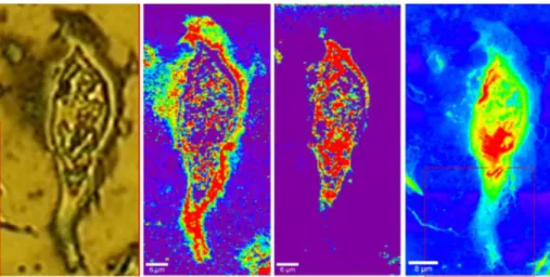
Differently from FITR, the use of Raman spectroscopy for cell imaging has been gaining greater and greater consideration. In brief, Raman spectrum origins from inelastic scattering of incident photons on the sample surface. As opposed to vibration which requires changes in dipole moment, Raman scattering requires a change in polarizability. As final result, Raman spectroscopy returns a spectral information that is similar but, in many cases, complementary to IR spectra. The Raman effect is very weak because only a tiny fraction of incident photons undergoes Raman scattering. Nevertheless, Raman spectroscopy and thus Raman microscopy possesses many advantages compared to FTIR imaging. In fact, both inorganic and organic compounds have a Raman spectrum and they usually return bands that are sharp and specific from a chemical point of view. In addition, it is perfectly suitable for imaging live cells (Fig. 1.4) also due to its non-invasive properties. The combination of Raman spectroscopy with confocal microscopy allows for lateral and vertical resolution of 250 nm and 1µm respectively.
14 State of the Art
Due to its sensitivity to C-H groups, Raman microscopy is considered the best option for imaging lipids in biological systems, but, unfortunately, the typical scanning time required (i.e., tenths of minutes on average) makes Raman spectroscopy not suitable yet for the analysis of the dynamic behaviours of cells and in particular, of intracellular structure and processes. The development of faster detectors would for sure greatly increase the applicability of this technique to many more biological situations and structures29.
1.3 Molecular information at the subcellular level from
fluorescence-based optical microscopy
None of the techniques described so far allows to extract molecular information at the subcellular level simultaneously in space and time, inside
Figure 1.4 Raman confocal microscopy example. Raman images obtained with a confocal
microscope at 250 x 250 nm2 spatial resolution. From left to right: optical image of the cell;
mapping of Raman shifts for lipids; phosphates and proteins. The red square in the image on the right was used for further analysis with AFM (not reported here). Image reprinted from ref.29
State of the Art 15
a living cell, at the proper resolution. They either entail the use of subcellular fractionation to isolate the structure/compartment of interest or they make use of sample fixation before measuring. An opportunity to tackle these issues comes in principle from fluorescence-based optical microscopy techniques. As a matter of fact, optical microscopy allows for the visualization of the molecules of interest (i.e., thanks to the use of fluorescent probes) inside living samples, by means of light sources in the UV-Vis- NIR range, that do not damage the sample and allow for prolonged imaging. Still, a major limit with optical microscopy techniques is represented by the diffraction limit of light that hinder the spatial resolution of the results (i.e., limited to around 250 nm). During the last decades, major efforts were made to overcome this limit. Super-resolution microscopy techniques were generated which allow fluorescence microscopy to push spatial resolution bypassing the diffraction limit imposed by visible light. Super-resolution microscopy represented such a breakthrough as a tool available to biologist and life science scientists that its inventors were awarded with Nobel prize for chemistry in 201431,32.
1.3.1 Localization-based methods: accuracy is a time-consuming task
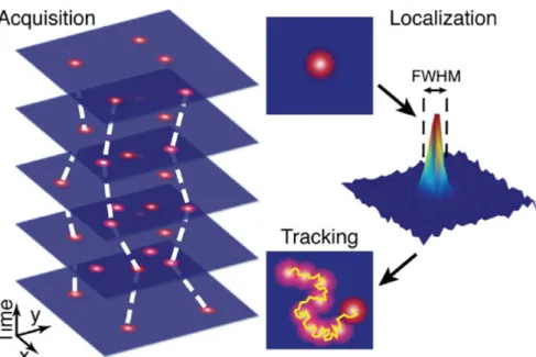
A classical example of localization-based methods is represented by single molecule/particle tracking (SMT/SPT). These approaches rely on a common principle. Nanoscopic reporters such as quantum dots, gold nanoparticles or fluorescent probes/molecules are attached to the biomolecule of interest and imaged several times (thus forming a stack of temporal images) using standard optical microscopy techniques. Every image is analyzed using different image processing algorithms that have the final purpose of determining the final spatial coordinates of the center positions of each imaged particle.
16 State of the Art
In each frame the positions of each particle are linked to the positions they possessed in the previous and following frames of the series (Fig. 1.5), thus allowing to unveil important parameters such as the mean square displacement (MSD).
Figure 1.5 Principle of standard SPT. A series of images containing the labelled molecules
of interest is acquired with a high-speed camera. The localization of the center-positions of each single molecule in each image of the series represents the core of the second step. These positions are then linked together between adjacent (in time) frames and trajectories of individual particles are generated. The displacement between two adjacent frames and the time elapsed between consecutive images give rise to the information about the dynamics of the observed objects. Image reprinted from ref.148
State of the Art 17
A fundamental requirement for localization-based microscopy is that the molecules/particles to be localized are sufficiently separated in space (i.e. the concentration is very low), a condition that is not always easy to obtain in biological experiments. Specific super-resolution approaches tackle this issue thanks to the use of photo-switchable/activable dyes or proteins (the general principle is explained in Fig. 1.6)33. These approaches were named stochastic
optical localization microscopy (STORM)34, photoactivated localization
microscopy (PALM)35 and fluorescence photoactivation localization
microscopy (fPALM)36. Fig. 1.7 shows the difference, for instance, between
the spatial resolution of conventional confocal microscopy and STORM34
applied at the subcellular scale.
These super-resolution approaches, in order to work properly, rely on the collection of multiple images of the same sample area (in each image a different subset of fluorophores is activated). Typically, thousands of images are needed to generate the final super-resolved one. This may take up to several minutes, while many cellular processes (included those at the subcellular level which are of interest here) happen on a much shorter timescale37,38 and requires a large amount of photons to be flashed on the
sample. Also, even in its simplest configuration, the localization process per
se is inherently limited by the time needed to acquire the number of photons Figure 1.6 Principle of localization microscopy. Different spatially separated fluorescent
probes are activated in different acquired image (thus at different time point). This avoids spatial overlapping of the active fluorophores and thus allows for their precise localization. After a long series of acquisition, a super-resolved image is reconstructed (right).
18 State of the Art
required for proper localization, and this in turn is linked to the choice of the fluorescent probe. Overall, localization-based techniques hit a limit at a resolution of about 10-20 nm.
Worthy of mention in this regard, Balzarotti et al. recently described another way of localizing single molecules called MINFLUX39. As in PALM and
STORM, fluorophores are stochastically switched on and off, but the emitter is located using an excitation beam that is doughnut-shaped, as in stimulated emission depletion. Finding the point where emission is minimal reduces the number of photons needed to localize an emitter. MINFLUX attained ~1-nm precision, resolving molecules only 6 nanometers apart. MINFLUX tracking of single fluorescent proteins increased the temporal resolution and the number of localizations per trace by a factor of 100, as demonstrated with diffusing 30S ribosomal subunits in living Escherichia coli. As conceptual limits have not been reached, the authors expect this localization modality to break new ground for observing the dynamics, distribution, and structure of
Figure 1.7. STORM imaging. Comparison of conventional confocal microscopy (left) and
STORM (right) imaging of microtubules and clathrin-coated pits (CCP). Image reprinted from ref. 33
State of the Art 19
macromolecules in living cells and beyond. Still, the ability of such strategy to discriminate between the dynamics of the structure of interest (the subcellular trafficking structure/organelle) and that of the biological processes occurring within the same structure has yet to be proven.
1.3.2 Structured illumination microscopy (SIM)
An alternative super-resolution approach not based on localization is Structured Illumination Microscopy (SIM). In brief, SIM exploits patterned light illumination to make high spatial frequencies available. A finely structured grating is placed on an intermediate image plane of a light widefield microscope that has the effect of projecting an illumination pattern through the optical path of the microscope on the sample surface38,40–42. The grating is
characterized by a single spatial frequency that induce interference in the recorded image. This interference allows the spatial frequency information to be shifted down to lower frequencies; in this way the high frequency information previously too high to be collected is now available in the resulting image. SIM is particularly suitable for live-cell imaging and large areas of the sample can be imaged thanks to its implementation in wide-field microscopes but, unfortunately, can provide an improvement in resolution by only a factor of two38. The main drawback, along with the relatively poor
spatial resolution, is represented by its relatively slow acquisition mode. The need to acquire multiple images of the same sample region requires obviously more time and this, in turn, implies the need for slow movements and low bleaching within the sample37,38. Given that, SIM remains suitable for live cell
imaging, and experimental data demonstrated the possibility to obtain a single image reconstruction in a time range that spans from few seconds to hundreds of milliseconds43,44. Fig 1.8 shows the comparison between the results
20 State of the Art
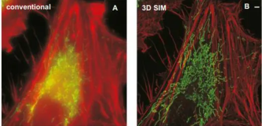
originating from the imaging of labeled mitochondria using both standard confocal microscopy and 3D-SIM45.
1.3.3 Stimulated emission depletion microscopy (STED)
Proposed in 1994 by Hell and colleagues46, the STED approach affords
increased spatial resolution by shaping the observation spot of the laser well below the standard diffraction limit. The principle is easy to explain: molecules brought to the excited state by a first laser excitation can be brought to the ground state before spontaneous fluorescence emission occurs if a second laser, matching the energy difference between the excited and ground states, is used 33,37,46,47. If the laser used to achieve stimulated emission
presents a pattern with zero intensity at the center, this can be adopted to shrink the excitation PSF by simply forming an annulus that prevents spontaneous emission in the illuminated region. In this case, to achieve super-resolution, the region in the center of the annulus, where spontaneous
Figure 1.8 Live 3D SIM imaging of labelled mitochondria. Live 3D SIM imaging of
mitochondria labelled with MitoTracker Green and the actin cytoskeleton labeled with tdTomato-LifeAct in a HeLa cell over 30 time points. (A) image taken using conventional microscopy. (B) 3D-SIM reconstruction of the same ROI shown in (A).Image reprinted from ref. 45
State of the Art 21
emission is allowed, must be smaller than the PSF of the laser use to have spontaneous emission33. To ensure that all spontaneous fluorescence emission
is prevented, STED laser intensity must reach a certain threshold which may damage the sample itself; in addition, raising the power of the STED laser allows to expands the depletion zone without particularly affecting the fluorescence spontaneous emission area. The size of this region is only limited by practical physical issue, related to the practical power of the STED laser33.
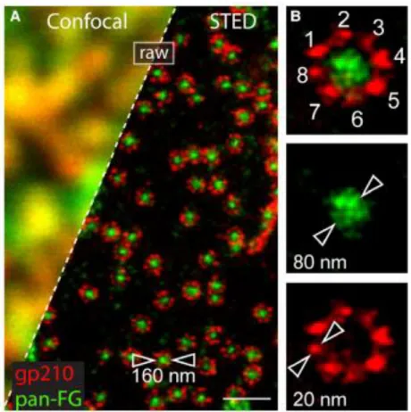
Figure 1.9 STED imaging of NPC. Comparison of conventional confocal microscopy and
STED. In this particular case, (A) STED reveals immulabeled subunits in amphibian NPCs. (B) Individual NPC showing eight antibody-labeled gdp12 homodimers as 20-40 nm size units and a 80 nm-sized localization of the subunits in the central channel. Image reprinted from ref.149
22 State of the Art
Fig. 1.9 shows a series of Nuclear Pore Complexes (NPCs) imaged first with a standard confocal microscope (above) and later using STED (below)48.
A major advantage achieved with STED microscopy is represented by the ability to deliver simultaneously high spatial and, potentially, temporal resolution. As a matter of fact, STED acquisition-time depends exclusively on the speed of the raster scan of the laser and the pixel dwell time used. Regard to this, important implementations were recently proposed. For instance, Schneider and co-workers successfully combined STED-based imaging with electro-optical scanning technologies to obtain an unprecedented line-scanning frequency of 250 kHz. Using SPT and taking advantage of the 70-nm static spatial resolution provided by STED, these authors investigated the dynamics of fluorescently labeled vesicles in living Drosophila or HIV-1 particles in cells with a temporal resolution of 5–10 ms49. More recently,
Lanzano and coworkers integrated STED with Fluorescence Correlation Spectroscopy (FCS) as a tool to look at molecules, and with two additional analytical approaches, the separation of photons by lifetime tuning (SPLIT) and the fluorescence lifetime correlation spectroscopy (FLCS), to efficiently and simultaneously probe diffusion in a 3D environment at different sub-diffraction scales50. SPLIT-FLCS combination allowed probing, from a single
FCS experiment, the diffusion from uncorrelated background, and continuously decreasing-in-size observation volumes in the cell cytoplasm, down to the spatial scale of approximately 80 nm, were reached. As a matter of fact, the authors proved the ability of STED-FCS-SPLIT-FLCS to generate the molecular diffusion laws at each single point in the cell at a relatively short spatiotemporal scale50. Worthy of mention here, FCS used as a tool to achieve
single molecule sensitivity (with no need to dwell on or localize any molecule in particular) offers an ideal platform to increase the temporal resolution and the overall performances of available optical microscopy techniques (see also next section).
State of the Art 23
1.4 Fluorescence Correlation Spectroscopy: a powerful tool to
boost the spatiotemporal resolution of optical microscopy methods
FCS represents a powerful tool to obtain information about the dynamics of molecules within living cells. In general, FCS is based on the autocorrelation of the fluorescent signal collected from fluorescent molecules contained in the sample; it provides the average diffusion time of the molecules contained in the observation volume and their average number. FCS and its various applications turned out to be particularly useful for the analysis of fluorescent molecules diffusing in the 3D intracellular environment (e.g. the cytosol) or on 2D biological membranes51–56.Figure 1.10 Principle of single-point FCS. The PSF of laser (green ellipsoid; this shape has
been selected to highlight the fact that the axial dimension of the PSF in a confocal microscope is higher the lateral dimension) is focused on a diffraction-limited point in the sample volume (left); fluorescent molecules (red dots) diffuse in the volume of the samples; some of them will enter and some will exit the volume of the PSF. The fluorescent emission generated inside the PSF is collected and converted into an electric signal (center); autocorrelation function is then computed using the equation shown in the middle where G(τ) represents the autocorrelation, τ the time lag, t the actual time of the electric signal and F(t) the electric signal originated from the fluorescence emission. Once the autocorrelation function is obtained (right) it is fitted to obtain the average number of particles inside the observation volume or the PSF (inversely proportional to G(0)) and the average diffusion coefficient D of the molecules that passed through the PSF during the acquisition time. Image adapted from ref.53
24 State of the Art
To introduce its general principle, single-point FCS approach is taken as a paradigmatic example. In single-point FCS, the laser of a common confocal microscope is focused on single point within a solution (e.g. the cell cytosol) containing the fluorescent molecules of interest (Fig. 1.10). The fluorescence emission is collected through a light detector such as a PMT and converted into an electric signal and, in turn, its autocorrelation function is calculated. By fitting the autocorrelation function with a model curve allows for the determination of the average diffusion and the average number of the molecules contained in the PSF53.
An important evolution of single-point FCS is the so called raster image correlation spectroscopy (RICS) technique57–60. RICS is a powerful tool since
it exploits the movement of the PSF during a confocal microscopy acquisition. As depicted in Fig. 1.11, in RICS, a spatial autocorrelation between adjacent pixels is performed59.
Figure 1.11 RICS principle. RICS represents a powerful tool since it exploits the
autocorrelation between fluorescence signals recorded in time by adjacent pixels. In this situation a raster scan acquisition of a typical confocal microscope is assumed. (Situation 1,
left) If a particle is fixed or slowly moving, its signal will be detected in pixels 1, 2 and 3 but
not in 4 during a line acquisition. The spatial autocorrelation will then reveal a slower motion of the particle (right, slower diffusion). (Situation 2, center) if a particle is moving quickly, there is a higher probability that it will be detected also in pixel 4 and this will then be visualized on the autocorrelation function (left, faster diffusion). Obviously, the correlation of the fluorescence at different pixels of distance will be dependent on the size of PSF of the laser adopted as well. Image reprinted from ref.59
State of the Art 25
The fitting of the spatial autocorrelation function again returns information regarding the dynamics of the fluorescent molecules under investigation. Of note, if multiple scan speeds image correlation spectroscopy of fluorescence fluctuations are used (as presented by Groner and collaborators61) each scan
speed can be used as a filter to select the characteristic temporal scale of molecular diffusion that significantly contributes to the measured correlation function. This approach can cover a wide dynamic range, as determined by available pixel dwell times, from below 1 µs to several milliseconds, and give selective access to average molecular displacements much smaller than the diffraction limit.
Figure 1.12 Mean Square Displacement analysis (MSD) obtained using RICS of GFP protein in the cell cytoplasm. Here the MSD of GFP protein contained in cell cytoplasm is
shown in comparison to the MSD of GFP in solution. The authors found evidence, using RICS, that, for short spatial scales (less than 100 nm), free GFP was diffusing in the cytoplasm as if it was diffusing in water; thanks to this result, the authors were able to demonstrated the presence of water within the cell; a theory that, even if obvious, until that moment was in contrast with experimental data. Image adapted from ref.60
26 State of the Art
My colleagues at NEST used this approach to study the dynamics of a paradigmatic inert, nanoscopic molecule (i.e. GFP) in the cytoplasm of living cells as compared with dilute solutions. Thanks to this comparison, they proved short-range, unobstructed, Brownian protein translational motion within the cytoplasm at the temporal scale from 10-6 to 2x10⁻⁵ sec,
corresponding to protein mean displacements from 25 to 100 nm60 (Fig. 1.12).
This was possible thanks to the high temporal resolution achievable with standard confocal microscope.
At the beginning of my PhD, such a platform appeared ideal to show how spatiotemporal fluctuation analysis can push the dynamic spatial resolution of a measurement well below the imaging nominal resolution, thus shedding light on unexplored dynamic phenomena such as the behavior of fluorescently labeled molecules trapped inside a vesicle.
To illustrate this, my colleagues had already performed a simulated experiment in which fluorescent molecules can move within a vesicle that is comparable in size to the static spatial resolution of the measurement (Fig.1.13). The simulated image series is used to reconstruct the iMSD profile of fluorescent molecules. Fig. 1.13 shows that by means of spatiotemporal fluorescence correlation spectroscopy, one can access the motion of fluorescent molecules trapped within moving vesicles and thus fully exploit information collected on timescales up to microseconds, which can be easily reached in a line-scanning acquisition with the aforementioned technology. In more detail, the iMSD plot displays two different diffusive regimes: a short-range diffusion that quantitatively describes the motion of molecules within the vesicle, and a 10-fold slower, long-range diffusion that reflects the movement of the entire vesicle. Both of these regimes match the imposed values. What is of importance here is that by applying spatiotemporal fluctuation analysis, we can resolve the dynamic behavior of molecules within
State of the Art 27
a submicrometric environment with a dynamic spatial resolution much higher than the nominal static spatial resolution set by the experimental conditions.
The idea to bring these potentialities into real experiments in living cells represents the starting motivation of my Thesis work..
Figure 1.13 Spatiotemporal fluctuation analysis can super-resolve single molecule dynamics: a simulated experiment. A three-dimensional moving spherical object (in this
case, a vesicle) with a diameter corresponding to the nominal measurement resolution (PSF) is filled with fluorescent molecules (see drawing in the inset). Both the vesicle and the molecules are free to diffuse, but the latter are 10 times faster than the vesicle and cannot cross the imposed spherical boundary. By applying spatiotemporal analysis of fluorescence fluctuations, one can measure the motion of the molecules within the vesicle (red dashed line) and the motion of the vesicle (blue dashed line) concomitantly, even if both are significantly smaller than the nominal imaging resolution. Image adapted from ref.55
Chapter
2
___________________________________________________________________
2.
Time-tunable Raster Image Correlation
Spectroscopy to capture molecular diffusion
in dynamic subcellular nanostructures
2.1 Time-tunable RICS on dynamic subcellular nanosystems
As the name suggests, RICS exploits the raster scan movement of the laser beam, as in the case of a confocal microscope for instance; in RICS the signal originated by adjacent pixels in a frame is correlated (see below for more details)58,59. This allows users to follow the motion of fluorescent moleculesthat move along adjacent pixels with an average time comparable to the motion of the laser beam, which is usually in the microsecond regime. Thus, a longer pixel dwell time will result in the detection of slower probes and vice versa. Spatiotemporal Image Correlation Spectroscopy (STICS), instead,
30 Time-tunable RICS
considers the spatiotemporal correlation of pixels separated by different frames in a temporal stack of images collected. This reveals the motion of even slower fluorescent entities that change position among consecutive temporally separated frames62. With STICS, millisecond-sampling periods are
obtained, unveiling the motion of entire intracellular compartments such as lysosomes or mitochondria. Starting from a theoretical work conducted by Di Rienzo et al. 60, we applied simple RICS analysis to study the motion of
molecules inside intracellular moving compartments, representing, as far as we know, both a novelty in the field, and a potential and easy tool to be adopted in the study of nanoscopic compartments of biological interest.
2.1.1 RICS analysis
The temporal stacks of images acquired for every experimental situation were first filtered using a moving average filter that eventually subtracted to each frame the values resulted from averaging the same frame with the following ones in the temporal sequence; this allowed removing the contribution to the signal of the immobile components of the acquisition. Once the filtering procedure was completed, image stacks were analyzed using RICS technique57–59.
The correlation curves derived from each experimental setup and each pixel dwell time were calculated on every image of the stack using Eq. 1:
𝐺(𝜉, 𝜓) =
〈𝐼(𝑥,𝑦)𝐼(𝑥+𝜉,𝑦+𝜓〉〈𝐼(𝑥,𝑦)〉 𝑥,𝑦 𝑥,𝑦2
(Eq. 1)
where I is the intensity of the pixel at the coordinates x (horizontal axis of the carpet) and y (vertical axis); ξ and φ are the spatial increments in the x and y direction respectively. Square brackets indicate the average operation over all
Time-tunable RICS 31
spatial coordinates (i.e., x and y). For each image stack, an average correlation (or RICS) curve was obtaining from the correlation curves of each image of the stack.
RICS curves were obtained from experimental acquisitions and these curves were fitted using the spatial correlation equation for normal raster scan acquisition57:
𝐺(𝜉, 𝜓) =
𝛾 𝑁(1 +
4𝐷(𝜏𝑝𝜉+𝜏𝑙𝜓) 𝑤02)
−1(1 +
4𝐷(𝜏𝑝𝜉+𝜏𝑙𝜓) 𝑤𝑧2)
−12) (Eq. 2)
where D is the diffusion coefficient, is the pixel dwell time while τl is the time
between lines in the single frame; w0 and wz are respectively the planar and
axial waists of the laser beam profile. Due to the possible variation in the laser alignment from day to day, the waist (w0) of the excitation beam was
calibrated before each day’s measurements as previously described by Digman et al.57. The fitting of the experimental curve with Eq. 2 allowed us
to find the diffusion coefficient (D) of the analyzed fluorophores.
The Stoke-Einstein equation (Eq. 3) was necessary to derive either the hydrodynamic radius or the solvent viscosity from diffusion measurements:
𝐷 = 𝑘𝐵𝑇
6𝜋𝜂𝑟 (Eq. 3)
2.1.2 STICS analysis
The temporal stacks of images acquired for every experimental situation were analyzed using STICS technique62. The correlation curves derived from each
32 Time-tunable RICS
experimental setup were calculated only for temporal stacks collected at 2µs pixel dwell time following Eq. 4:
𝐺(𝜉, 𝜓, 𝜏) =
〈𝐼(𝑥,𝑦,𝑡)𝐼(𝑥+𝜉,𝑦+𝜓,𝑡+𝜏〉〈𝐼(𝑥,𝑦,𝑡)〉 𝑥,𝑦 𝑥,𝑦2
(Eq. 4)
where I (x,y,t) is the intensity of the pixel at the coordinates x,y at time t; ξ and φ are the spatial increments in the x and y direction respectively and τ is the temporal lag between consecutive frames in the same temporal stack. In this particular case, we used temporal stacks acquired at 2µs pixel dwell time with 33 nm pixel size and 128 x 128 pixel resolution. This results in a time lag between two consecutive frames in a stack of 188 ms. Square brackets indicate the average operation over all spatial coordinates (i.e., x and y). For each image stack, a STICS curve was obtained and fitted following standard equations already described elsewhere63. This analysis returned the diffusion
coefficients (D) of the motion of objects corresponding to a sampling period of 188 ms. It is important to stress that the employment of RICS alone would be sufficient to unveil the dynamic behaviour of both subcellular organelles and their molecular species contained within, but, nonetheless, the use of STICS will open to the possibility of analysing the movement of subcellular compartments to a lager temporal scales (compatible with the scales of other SPT techniques) thus allowing for a complete analysis of their behaviours simultaneously.
Time-tunable RICS 33
2.1.3 Time-tunable RICS validation on dynamic nanosystems in vitro
For the validation of this time-tunable FCS on nanoscopic vesicles, a set of experiments that could prove its reliability was conducted. Quantum dots (QDs) were selected as testing probes thanks to their high signal to noise ratio regarding fluorescence emission. RICS was initially performed on QDs simply dispersed in their buffer solution and average diffusion coefficients were extracted for every pixel dwell time (Fig. 2.1 and 2.2).
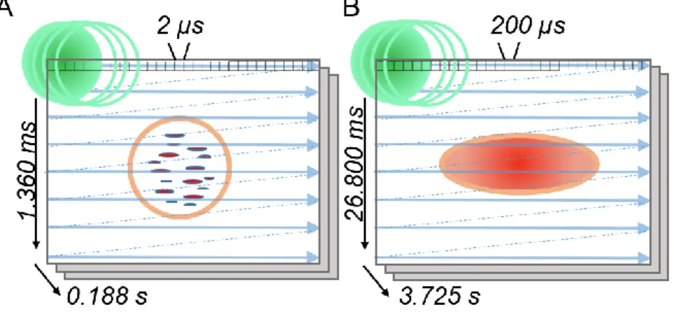
Figure 2.1 Time-tunable RICS principle. Schematic representation of the main concepts
underlying the technique. (A) The use of short pixel dwell time (e.g., 2 µs that translates in 1.360 ms of line time and 0.188 s of frame time) unveils the motion of fluorescent molecules inside intracellular compartments. (B) With long pixel dwell time ((e.g., 200 µs that translates in 26.800 ms of line time and 3.725 s of frame time) the motion of the compartment is more and more dominant in the overall result.
34 Time-tunable RICS
To simulate intracellularly moving vesicles, QDs were loaded inside liposomes, and they were then poured in an agarose solution to be slowed down. Temporal stacks of confocal images were collected at different pixel dwell time and correlation curves were obtained and fitted (Fig. 2.2). Diffusion coefficients were then extracted as for the previous experiment.
Figure 2.2. Pixel dwell time comparison. (A) Illustrative frame collected at 2 µs showing a
liposomes containing QDs (left) and its corresponding RICS curve (right with color scale bar: red represents the highest value and dark blue the lowest). (B) Illustrative frame collected at 200 µs showing the same liposome containing QDs reported in A (left) and its corresponding RICS curve (right with color scale bar: red represents the highest value and dark blue the lowest). Notice how RICS curve corresponding to 200 µs is broaden if compared with the 2 µs curve. This is explained by the detection of faster movements in the acquisition reported in A. (C) Real (above) and fit (below) RICS curves of the acquisition reported in A. (D) Real (above) and fit (below) RICS curves of the acquisition reported in B. Notice how RICS curve in D is broader than the curve reported in C. Again, this is due to the selection of slower motional behaviors of the acquisition in D compared to the faster ones collected in C.
Time-tunable RICS 35
As Fig. 2.3 shows, with a fast scan speed we were able to select and analyze the motion of fast molecules inside moving organelles, while, as the scan speed slows down, the motion of the compartment itself becomes more and more relevant in the outcome of the correlation (Fig. 2.1A and B). For this reason and in order to analyze all possible motions inside intracellular compartments, temporal stacks of confocal images were acquired at different pixel dwell times, namely at 2, 4, 8, 20, 40, 100 and 200 µs.
Figure 2.3 Diffusion coefficients of QDs within liposomes at different pixel dwell times.
This graph shows the Diffusion coefficients found for both QD-loaded liposomes (black dots) and QDs in buffer solution (white dots) at different sampling time. Note the distinction between RICS and STICS time domains. Below the data, we reported a schematic representation of the situation studied at different time samplings. On the left, thus for short pixel dwell times (few microseconds) we find a situation in which RICS analysis reveals movement of the molecules inside the liposome. As we move towards longer sampling times (hundreds of microseconds), the situation is a sort of mixture between the molecular movements and the displacements of the entire structure; until, for STICS time domains (hundreds of milliseconds), only the displacement of the entire compartment sticks out in the correlation analysis.
36 Time-tunable RICS
These stacks were then analyzed using RICS and STICS and diffusion coefficients at different sampling time were extracted by fitting the obtained correlation curves with the equations provided above in section 2.1.1 and 2.1.2.
As Fig. 2.3 reports, diffusion coefficients of QDs inside liposomes (black dots) follow the values of the coefficients of free QDs (blue dots) for short pixel dwell time (2, 4 and 8 µs). As pixel dwell time increases, the motion of the overall liposome prevails in the correlation analysis and diffusion coefficients start decreasing until they reach the value of the coefficient of the sole liposome found with STICS analysis (188 ms). It is worth to mention that diffusion coefficients of free QDs are reported only for RICS analysis, since it is impossible with STICS to recover their full diffusivity due to the down-sampling limit of the technique.
To further prove the reliability of this technique we compared the diffusion coefficients obtained at 4 µs of pixel dwell time with the coefficients found on the same samples using feedback-based 3D Orbital Tracking (OT) technique combined with RICS (this is a really complex technique that will be the object of the following Chapters; for this reason and for a detailed description the reader is redirected to Chapters 3 and 4; within this particular experimental work, the technique was simply adopted as a control experiment). As described in Chapter 3, OT is a feedback-based tracking technique that moves an excitation light beam along an orbit surrounding the fluorescently labeled structure of interest (in our case a QD-loaded liposome). Analyzing the collected fluorescence signal of OT with RICS allowed us to recover the diffusion coefficients of the fluorescent probes (QDs in this case) and the motion of the overall tracked structure (the QD-loaded liposome in this second case). The values obtained with OT were comparable to the coefficients obtained using RICS and STICS (see Fig. 2.4).
Time-tunable RICS 37
2.1.4 Time-tunable RICS validation in biological samples
The lysosome is selected as a paradigmatic case study. HeLa cells were cultured in physiological conditions and treated with Red Lysotracker (Fig. 2.5); this fluorescent dye was selected as it proved to be prone to the analysis of molecule diffusion in combination with FCS64. Stacks of images at 33 nm
of pixel size were collected under a confocal microscope at different sampling times. Again, acquisitions were done at 2, 4, 8, 20, 40, 100 and 200 µs of pixel dwell time and data were analyzed using RICS and STICS (Fig. 2.5 and 6).
Figure 2.4. Control experiments with Orbital Tracking on QD-loaded liposomes. (A)
Example of a QD-loaded liposome trajectory in agarose gel obtained using 3D orbital tracking. The average Diffusion coefficient of liposomes slowed down in Agarose gel is 0.085 ± 0.047µm2/s (expressed as mean ± standard deviation). Ticks on axes represents pixels, thus 50
nm of space distance. (B) Plot of the diffusion coefficients of both QDs dispersed in Borate buffer (red) and QD-loaded liposomes in Agarose gel (green) measured obtained with Orbital Tracking using 4 µs of pixel dwell time. Upper and lower edges of the boxes represent the 25 and 75 percentiles of the distributions found; the middle line shows the mean value. Whiskers show standard deviations.
38 Time-tunable RICS
The analysis returned diffusion coefficient values decreasing in time as for the case of QD-loaded liposomes (Fig. 2.3).
Using the Stoke-Einstein equation (Eq. 3 section 2.1.1), and assuming a hydrodynamic radius of 0.8 nm for Red Lysotracker inside lysosomes, we
Figure 2.5 Red Lysotracker in lysosomes of HeLa cells. (A) Confocal image of a HeLa cell
labelled with Red Lysotracker (scale bar 10 µm). (B) Magnification of figure A, white square. This is the magnification used for time-tunable RICS experiments (i.e., 33 nm per pixel).
Figure 2.6 Diffusivity of Red Lysotracker in lysosome of HeLa cells. This graph shows the
Diffusion coefficients of Lysotraccker inside lysosomes of HeLa cells different sampling time. Notice the distinction between RICS and STICS time domains.
Time-tunable RICS 39
extrapolated an average lysosome viscosity of 73 cP that is line whit what previously showed in literature by Wang et al65.
Measurements on free Alexa488 in solution were also acquired as a control experiment (Fig. 2.7), resulting in much higher diffusion coefficients as expected when compared to Lysotracker inside lysosomes.
Unfortunately, there is no obvious way to determine the hydrodynamic radius of Red Lysotracker inside lysosomes, due to the acidic condition and the crowded environment that characterize lysosomes.
Figure 2.7 Comparison between diffusion coefficients of free Alexa 488 dissolved in water and of Red Lysotracker in lysosomes of HeLa cells. This graph shows the Diffusion
coefficients found for both free Alexa 488 dissolved in water (green dots) and Red Lysotracker (red dots) contained in the lysosomes of HeLa cells at different sampling time. Notice how free Alexa returns diffusion coefficients that are two order of magnitude higher than Lysotracker; both Alexa and Lysotracker are small molecule with comparable hydrodynamic radius, but Alexa is diffusing in a much less viscous environment (i.e., pure water). We highlight the fact that after 20 µs of pixel dwell time the diffusion coefficients of Alexa start decreasing due to a down-sampling condition; dueto high diffusivity of Alexa it becomes impossible to follow its rapid movements using long sampling period; it is a physical limit.
40 Time-tunable RICS
It is worth to highlight that more than a viscosity value, time-tunable RICS affords a measurement of the ‘apparent’ diffusion coefficient. I deliberately used the word ‘apparent’ because the diffusion coefficient strictly depends on the sampling time at which the acquisition is performed. Thus, comparing diffusion coefficients extrapolated with the same pixel dwell-time is mandatory. Still, based on the fact that the diffusivity (and thus the viscosity) obtained by RICS is in good agreement with the results reported before by Wang et al.65 (obtained by a completely different strategy: lifetime applied to
an activatable rotor probe), we are prompted to speculate that our estimates are close to the real viscosity of the organelle. In addition, feedback-based 3D OT, as shown in the next Chapter can afford a similar estimate of the average diffusion coefficient of the organelle itself. In addition, the average value found using STICS and Lysotracker (i.e., 0.012±0.007 µm2/s, mean ± SD)is
also close to the results obtained by Digiacomo et al.66 on HeLa cells treated
with Lysotracker using iMSD, a technique close to the STICS proposed herein.
Figure 2.8 Diffusivity of Red Lysotracker and GFP-labeled CD63. Plot of the diffusion
coefficients of Red Lysotracker (red) and GFP-labeled CD63 (green) measured on lysosomes of HeLa cells obtained at 2 µs of pixel dwell time. Upper and lower edges of the boxes represent the 25 and 75 percentile of the distributions found, the middle line shows the mean value. Whiskers show standard deviations (left side). Schematic representation of the two distinct situations (right side).
Time-tunable RICS 41
To provide additional support to the reliability of this application, we again conducted the analysis on lysosomes, but, this time, using a different
Figure 2.9 Control experiments for GFP-labelled CD63 protein. To further prove the
reliability of the measured values of CD63 protein in HeLa cells, we conducted control experiments where we measured diffusivity of both free GFP in water and Rhodamine-labeled DOPE lipid in liposomes. In this latter case, liposomes were formed as a mixture of lipids: Rhodamine-labeled DOPE and DPPC (see Appendix B). (A) This graph shows the Diffusion coefficients found for both free GFP dissolved in water (light green dots) and GFP-labeled CD63 on lysosomes of HeLa cells (dark green dots) at different sampling time. Notice how free GFP, as for Alexa 488 above, returns diffusion coefficients that are almost two order of magnitude higher than Lysotracker; both free GFP and CD63 are small proteins with comparable hydrodynamic radius, but free GFP is diffusing in a much less viscous environment (i.e., pure water). (B) Here the graph shows the diffusivity of both CD63 in HeLa cells (green dots) and Rhodamine-labeled liposomes (red dots). We found different diffusivities especially for short pixel dwell times where the molecular diffusion gives a higher contribution to the correlation curves. The analysis returned that Rhodamine-DOPE diffuses on liposome surface much faster than CD63 does on lysosome surface as expected. In addition, as for the case of free GFP and GFP-alebelled CD63 protein reported in A, the rate of molecular diffusion of Rhodamine-DOPE showed a much slower behavior compared to free Rhodamine in solution as previously demonstrated150. The proposed method is also able to discriminate different