Movies and meaning: from low-level features to mind reading
Sergio Benini;Department of Information Engineering, University of Brescia; Brescia, Italy
Abstract
When dealing with movies, closing the tremendous disconti-nuity between low-level features and the richness of semantics in the viewers’ cognitive processes, requires a variety of approaches and different perspectives. For instance when attempting to relate movie content to users’ affective responses, previous work sug-gests that a direct mapping of audio-visual properties into elicited emotions is difficult, due to the high variability of individual re-actions. To reduce the gap between the objective level of features and the subjective sphere of emotions, we exploit the intermediate representation of the connotative properties of movies: the set of shooting and editing conventions that help in transmitting mean-ing to the audience. One of these stylistic feature, the shot scale, i.e. the distance of the camera from the subject, effectively regu-lates theory of mind, indicating that increasing spatial proximity to the character triggers higher occurrence of mental state refer-ences in viewers’ story descriptions. Movies are also becoming an important stimuli employed in neural decoding, an ambitious line of research within contemporary neuroscience aiming at “mind-reading”. In this field we address the challenge of producing de-coding models for the reconstruction of perceptual contents by combining fMRI data and deep features in a hybrid model able to predict specific video object classes.
Introduction
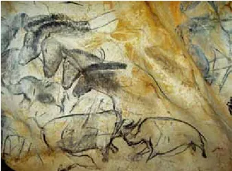
Cinema is definable as the performing art based on the op-tical illusion of a moving image. Despite cinema movies owe its mass spread by invention of the Lumiere brothers’ cinemato-graph, humans have been always using the figurative arts to rep-resent images of the world around them. Some studies attribute the cinema authorship even to Palaeolithic paintings [1] as they represent scenes of animals not in a statical pose but rather dy-namically providing the illusion of moving objects, as in famous cave of Chauvet-Pont-d’Arc (see Figure 1).
The 'scienti c' role of cinema
Movies are not only one of the most known entertainment sources but have become, in the last half century, one of the pre-ferred testbed addressed by an increasing number of scientific studies. This happens because, while watching movies, the viewer often becomes a participant, because his entire body - his senses, his equilibrium, his imagination - are all convinced that an imag-inary event is really happening. Human intersubjectivity proper-ties, such as empathy [2] or theory of mind [3], allow viewers to immerse themselves in the film and experience similar mental and physiological states of the real life [4].
For this peculiarity, the analysis of movies and their con-tent is of particular interest in different areas of science, beyond Cinematography itself, such as Psychology and Neuroscience, al-though with different purposes: cognitive film scholars carefully
study various elements of the film viewing experience focusing on the mental activity of viewers as the main object of inquiry; psychologistsdescribe the phenomenology of the film experience to study affective processes and human relationships; neurosci-entistsrecently started using movie excerpts as controlled brain stimuli in brain imaging studies.
The interest towards movie data of tech disciplines such as Computer Visionor Image Processing, traditionally confined to applications such as automatic content analysis or video compres-sion, is nowadays expanding to the challenging aim of finding suitable representations of movie data useful for other disciplines to pursue their fundamental tasks. It is not a coincidence that sometimes the limit that separates these different areas of science becomes pretty blurry and that multidisciplinary approaches to the problems of semantics and cognition are seen as the most promis-ing ones, where movies are often the common denominator that bring all these areas together.
Methodologies and features
Despite a heterogeneity of objectives, traditional approaches to semantic video analysis have been rather homogeneous, adopt-ing a two-stage architecture of feature extraction first, followed by a semantic interpretation, e.g. classification, regression, etc.
In particular feature representations have been predomi-nantly hand-crafted, drawing upon significant domain-knowledge from cinematographic theory and demanding a specialist effort to be translated into algorithms.
Since few years however, we are witnessing a revolution in machine learning with the reinvigorated usage of neural networks in deep learning, which promises a solution to tasks that are easy
Figure 1. Panel with horses in the cave Chauvet - Pont d’Arc (Ardeche) c
J. Monney-MCC.
https://doi.org/10.2352/ISSN.2470-1173.2017.14.HVEI-117 © 2017, Society for Imaging Science and Technology
for humans to perform, but hard to describe formally. Deep learn-ing is a branch of machine learnlearn-ing based on a set of algorithms that attempt to model high level abstractions in data through stack-ing different layers, with more abstract descriptions computed in terms of less abstract ones [5].
While on the one hand-crafted features ensure full under-standing of the underlying processes and control over them, on the other hand deep learning methods are showing not only supe-rior ability to regress objective functions in most tasks, but also transfer learningcapability, that is when it is possible to build a model while solving one problem and applying it to a different, but related problem. Though appreciable in general, performance and transfer learning abilities may be not not always sufficient in order to validate the learnt models, as it happens for example in Neuroscience, where the method should also provide insights on the underlying brain mechanisms [6].
Tackling movie semantics
The rest of this work presents some studies and results of few years of research in semantic movie analysis. While pursu-ing this goal, different perspectives on the problem and diverse methodologies have been taken into account.
We first show how to extract low-level and grammar features related to style and link them to emotional responses gathered from the audience, and how to exploit these characteristics for recommending videos [7, 8]. We then focus on one of these stylis-tic features, the scale of shot, which Cognitive Film Theory links to the film’s emotional effect on the viewer [9] and propose auto-matic pipelines for its computation. Last we present a new hybrid approach to decoding methods employing deep learnt features, with the goal of predicting which sensory stimuli the subject is receiving based from fMRI observations of the brain activity [10]. Research questions
In short the studies presented in the following try to tackle the following research questions:
• Which methods are suitable for providing movie represen-tations useful for closing the tremendous discontinuity be-tween low-level features and the richness of semantics in the viewers’ cognitive processes?
• Can automatic analysis of stylistic features help in study-ing the impact on viewers in terms of attribution of mental states to characters and in revealing recurrent patterns in a director’s work?
• How effective is the combination of deep learnt features and fMRI brain data in decoding approaches to reveal perceptual content?
Being able to fully answer these questions rises the challenge provided by interdisciplinary learning, which has the ultimate goal of facilitating the exchange of knowledge, comparison and debate between apparently far disciplines of science [11].
For the presented studies, whenever possible, we also bring up the question whether hand-crafted features are sufficient to ob-tain an adequate representation of the movie content, or whether it is better to “deep” learn the movie content representation. Rather than providing ultimate answers, we show examples and coun-terexamples of different approaches and, maybe complementary, mindsets.
Connotation and lmic emotions
Emerging theories of filmic emotions [12][13] give some in-sight into the elicitation mechanisms that could inform the map-ping between video features and emotional models. Tan [12] sug-gests that emotion is triggered by the perception of “change”, but mostly he emphasises the role of realism of the film environment in the elicitation of emotion. Smith [13] instead attempts to re-late emotions to the narrative structure of films, giving a greater prominence to style. He sees emotions as preparatory states to gather information and argues that moods generate expectations about particular emotional cues. According to this, the emotional loop should be made of multiple mood-inducing cues, which in return makes the viewer more prone to interpret further cues ac-cording to his/her current mood. Smith’s conclusion that “emo-tional associations provided by music, mise-en-scene elements, color, sound, and lighting are crucial to filmic emotions”, encour-age attempts to relate video features to emotional responses. Motivation and aims
Previous work suggests that a direct mapping of audio-visual properties into emotion categories elicited by films is rather dif-ficult, due to the high variability of individual reactions. To re-duce the gap between the objective level of video features and the subjective sphere of emotions, in [7, 8] we propose to shift the representation towards the connotative properties of movies.
A film is made up of various elements, both denotative (e.g. the purely narrative part) and connotative (such as editing, mu-sic, mise-en-scene, color, sound, lighting). A set of conventions, known as film grammar [14], governs the relationships between these elements and influences how the meanings conveyed by the director are transmitted to persuade, convince, anger, inspire, or soothe the audience. As in literature, no author can write with color, force, and persuasiveness without control over connota-tion of terms [15], in the same way using the emoconnota-tional appeal of connotation is essential in cinematography. While the affective response is on a totally subjective level, connotation is usually considered to be on an inter-subjective level, i.e. shared by the subjective states of more individuals. For example, if two people react differently to the same horror film (e.g. one laughing and one crying), they would anyway agree in saying that that horror movie atmosphere is grim, the music gripping, and so on.
The main goals of this study are to verify the following hy-pothesis: i) whether connotative properties are inter-subjectively shared among users; ii) if they are effective for recommending content; iii) whether it is possible to predict connotative property values directly from audiovisual features.
The connotative space
In [7] we introduce the connotative space as a valid tool to represent the affective identity of a movie by those shooting and editing conventions that help in transmitting meaning to the audi-ence. Inspired by similar spaces for industrial design [16] and the theory of “semantic differentials” [17], the connotative space (see Figure 2) accounts for a natural (N) dimension which splits the space into a passional hemi-space, referred to warm affections, and a reflective hemi-space, that represents offish and cold feel-ings (associated dichotomy: warm vs. cold). The temporal (T) axis characterizes the space into two other hemi-spaces, one re-lated to high pace and activity and another describing an intrinsic
attitude towards slow dynamics (dynamic vs. slow). Finally, the energetic (E)axis identifies films with high impact in terms of affection and, conversely, minimal ones (energetic vs. minimal).
energetic / minimal cold / warm slo w / d ynamic Slo w / Dynamic Energetic / Minimal Cold / Warm Slo w / Dynamic Energetic / Minimal Cold / Warm
N
E
T
Figure 2. Connotative space for affective analysis of movie scenes.
Validation by Inter-rater Agreement
As a first advantage of using the connotative space, in [7] we show that the level of agreement among users is higher when rating connotative properties of the movie rather than when they self-report their emotional annotations (emo-tations).
The experiment is set up as follows. A total number of 240 users are recruited. Out of these, 140 fully completed the exper-iment, while others performed it only partially. The experiment is in the form of a user test and it is performed online. Data con-sist of 25 “great movie scenes” [18] below 3 minutes of duration (details in [7]), representing popular films spanning from 1958 to 2009 chosen from IMDb [19] (in Figure 3, a representative key-frame for each scene is shown). To perform the test, every user is asked to watch and listen to 10 randomly extracted movie scenes out of the total 25, in order to complete the test within 30 minutes. After watching a scene, each user is asked to express his/her annotations. First the user is asked to annotate his/her emotional state on the emotation wheel in Figure 4-a. This model is a quan-tized version of the Russell’s circumplex and presents, as in the Plutchik’s wheel, eight basic emotions as four pairs of semantic
1 2 3 4 5
6 7 8 9 10
11 12 13 14 15
16 17 18 19 20
21 22 23 24 25
Figure 3. Representative key-frames from the movie scene database.
opposites: “Happiness (Ha) vs. Sadness (Sa)”, “Excitement (Ex) vs. Boredom (Bo)”, “Tension (Te) vs. Sleepiness (Sl)”, “Distress (Di)vs. Relaxation (Re)”.
d=1 d=2 d=3 d=4 Relaxation Excitement Distress Boredom Sadness Happiness Sleepiness Tension Relaxation Excitement Distress Boredom Sadness Happiness Tension d=1 d=2 Sleepiness d=3 ei = 'Ha' a) b)
Figure 4. a) The emotation wheel used by users to annotate emotions; b) on the emotation wheel relatively close emotions are adjacent to each other.
Then users are asked to rate on a Likert scale from 1 to 5 three connotative concepts accounting for the natural, temporal and energetic dimensions of the connotative space. Ratings are expressed on three bipolar scales based on the semantic oppo-sites (see Figure 5): warm/cold (natural), dynamic/slow (tempo-ral), and energetic/minimal (energetic), respectively. In particular users are asked to rate: i) the atmosphere of the scene from cold to warm; ii) the pace of the scene from slow to dynamic; iii) the scene impact on them from minimal to energetic.
Tension Sleepiness 1 2 3 4 5 1 2 3 4 5 1 2 3 4 5 1 2 3 4 5 Cold Warm Slow Dynamic Minimal Energetic Sa Di Di Ha Re Sl Ex Di Te Bo Sa 1 2 3 4 5
Figure 5. The most voted 5 contiguous emotions of each scene (white sector) are turned into a five-level bipolar scale, thus comparable with the three scales related to the connotative properties of the scene.
As adopted scales are of the “interval” type, we assess the rater agreement by the intra-class correlation coefficient (ICC) [20], which statistically estimates the degree of consensus among users. Values of inter-rater agreement expressed for the three con-notative axes and for emotations are given in Table 1.
Agreement Emot. Natu. Temp. Ener. ICC(1, k) .7240 .8773 .8987 .7503 Measures of inter-rater agreement ICC(1, k).
The comparison between intra-class correlation coefficients clearly shows that the overall agreement is consistently higher when users are asked to rate connotative concepts of the movies rather than when they have to provide emotional annotations. Therefore the proposed space seems to fill the need for an interme-diate semantic level of representation between low-level features and human emotions, and envisages an easy translation process of video low-level properties into intermediate semantic concepts mostly agreeable among individuals.
Recommendation based on connotation
The second main outcome provided by analysis in [7] shows how connotation is intrinsically linked to emotions. In the specific we verify that in order to meet the emotional wishes of a single user it is better to rely on movie connotative properties, rather than to exploit emotations provided by other users. The hypothesis is that movie scenes sharing similar connotation are likely to elicit, in the same user, similar affective reactions.
The testing scenario uses the notion of ranked top lists. The idea is that the system returns, on the basis of the user request, a top list of items ranked in the connotative space, which are rele-vant to the user. Once the user expresses an emotional wish, using as a reference those scenes he/she has already emotated as rele-vant to that emotional wish, we produce two lists of suggested scenes, one in the connotative space and the other based on emo-tations by all users, as depicted in Figure 6. Both lists are ordered according to a minimum distance criterium in the corresponding space. To understand which space ranks scenes in a better or-der, we compare the two lists with a third one, considered as the best target, which is ranked based on the emotations stored in the user’s profile. Te Connotative Space User's Profile Emotation Wheel Movie Scenes
Target Top List
Connotative Top List
Emotation Top List Ex Te Ha Re User's Profile Ex Ha Re Te Tense Scene/s I want Tension Ranking by:
Figure 6. Given one emotional wish, movie scenes of the user profile are differently ranked in the connotative and emotation space. The two lists are compared with the best target provided by the user’s profile.
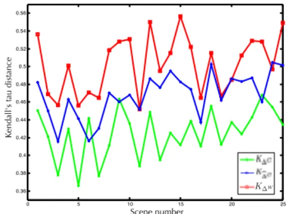
To compare lists in the connotative and emotation spaces with respect to the optimal lists, we adopt the Kendall’s tau dis-tance [21] which accounts for the number of exchanges needed in a bubble sort to convert one permutation to the other. Figure 7 shows the comparison between Kendall’s tau distances averaged on scenes, suggesting the superior ability of the connotative space in ranking scenes and approximating the optimal ranking.
Since connotative elements in movies strongly influence in-dividual reactions, the proposed space relates more robustly to single users’ emotions than using emotional models built on col-lective affective responses. By using the connotative space, be-yond obtaining a higher agreement in ratings among users, we are able to better target the emotional wishes of single individuals. Recommendation based on connotative features
While in [7] connotative rates are assigned by users, in the study in [8] we aim at predicting connotative values directly using audiovisual features. Figure 8 presents the modelling approach to establish a relation between connotative rates assigned by users and video characteristics. The descriptions of the main blocks follow. 0 5 10 15 20 25 0.35 0.4 0.45 0.5 0.55 0.6
Kendall tau distance
Scene number Kendall tau distance scene!based
Connotative space Emotations
Scene number
Kendall tau distance (scene based)
Figure 7. Distance K computed on a scene basis. Ranking in the connota-tive space better approximates in all scenes the optimal ranking.
SVR model Feature extraction 25 movie scenes Scene Rating Feature selection Users N T E
Scene distances based on connotative votes Scene distances based on features Δc ΔFi Support Vector Regression
Scene dist. based on selected features
Fi*
Δ
Figure 8. Diagram describing the modelling workflow.
Scene rating by users In [7] 240 users rated a set of 25 “great movie scenes” on the three connotative dimensions (N, T, E), where rates [1, 2, 3, 4, 5] are assigned on bipolar Likert scales based on the semantic opposites: warm/cold, dynamic/slow and energetic/minimal. After rating, the position of a scene mi in
the connotative space is described by the histograms of rates on the three axes HiN, HT
i , HiE
. Inter-scene distances between couples (mi, mj) are computed by using the Earth mover’s
dis-tance(EMD) [22] on the rate histograms of each axis (N, T, E) as ∆ xi, j= EMD (Hix, Hx
j), x ∈ { N, T, E} , which are then combined
to obtain the matrix of connotative distances between scenes as ∆ C= f
∆ N, ∆ T, ∆ E (where function f is set so as to perform a linear combination of the arguments with equal weights on the three dimensions).
Feature extraction From movie scenes we extract features dealing with different aspects of professional content: 12 visual descriptors, 16 audio features and 3 related to the underlying film grammar, as listed in Table 2.
Visual
dominant col., col. layout, scalable col., col. structure, col. codebook, col. energy, lighting key I, lighting key II, saturation , motionDS
Audio
sound energy, low-energy ratio, zero-crossing rate , spectral rolloff , spectral centroid , spec-tral flux , MFCC , subband distribution , beat histogram, rhythmic strength
Grammar shot length, illuminant col., shot scale change Extracted features ( = both average and standard deviation). Since each feature Fl is extracted at its own time scale
fea-ture histogram HFl
i to globally capture its intrinsic variability. For
each feature, matrices of inter-scene distances DFl are computed
as distances between feature histograms.
Feature selection To single out those features Fl that are the most related to users’ connotative rates, we adopt an informa-tion theory-based filter which selects the most relevant features in terms of mutual information with user votes, while avoid-ing redundant ones: the minimum-redundacy maximum-relevance scheme (mRMR) introduced in [23].
To compute mutual information it is necessary to sample probabilities of features and votes. However, when dealing with multidimensional feature histograms HFl, the direct application
of such procedure is impractical. To overcome this issue, for the selection and regression steps we do not take into account actual histograms, but distances between them. Therefore we do not employ the absolute position of scenes, but the knowledge of how they are placed with respect to all others, both in connotative and in feature spaces.
Following this procedure we finally select 4 features for the natural dimension, 3 for the temporal one and 2 for the energetic one. As expected, selected features for the natural axis are intu-itively involved in the characterization of a scene’s atmosphere: they in fact describe the color composition (color layout), the variations in smoothness and pleasantness of the sound (spectral rolloff standard deviation) and the lighting conditions in terms of both illumination (illuminant color) and proportion of the shadow area in a frame (one of the lighting key descriptors, dramatically stressed in the chiaroscuro technique). The algorithm returns for the temporal axis the rhythmic strength of the audio signal, which is an index related to the rhythm and the speed sensation evoked by a sound, the pace variation of the employed shot types (shot scale change rate), and the variability of the motion activity (stan-dard deviation on motion vector modules). Selected features on the energetic dimension are again commonsensical and coherent: the first describes the sound energy, while the second one is the shot length; for example short shots usually employed by direc-tors in action scenes are generally perceived as very energetic. Regression A support vector regression (SVR) approach relates connotative distances based on users’ rates DC to a function of inter-scene distances based on selected features DFl. By the learnt
SVR model, connotative distances can be predicted as bDC. Scene recommendation Once validated the model, we are able to predict connotative distances between movie scenes starting from distances based on selected features. To evaluate how good distances based on selected features bDC approximate scene dis-tances computed on users’ rates DC, we compare the abilities of the two distance matrices in ranking lists of movie scenes with respect to ground-truth lists built by single users. As done in Figure 7 ranking quality is again measured by the Kendall’s tau metric K [21] in the interval [0; 1]. Inspecting results in Figure 9 (which shows Kendall’s tau scores for each of the 25 scenes, as av-erage result on a five-folded evaluation) in a comparative way, we can conclude that even if the regression undeniably introduces an error, when the goal is not to replicate exact connotative distances but to obtain a similar ranking, the average ability of the system
does not significantly degrade when using bDCinstead of DC. More important, returned lists using bDCbetter match the ground-truth lists per each single user than using the aggregated annotations by other users DW, meaning that even connotative properties pre-dicted by audiovisual features are more inter-subjectively agreed among people than collective emotional annotations.
0 5 10 15 20 25 0.36 0.38 0.4 0.42 0.44 0.46 0.48 0.5 0.52 0.54 0.56
Kendall tau distance
Scene number Kendall tau distance scene!based
Scene number
Kendall's tau distance
*
K∆W
Figure 9. Kendall’s tau metric measuring the quality of list ranking by using connotative distances based on votes (KDC) and by distances approximated with the learning models (KbDC). Since the ground-truth lists are at K=0, both DCand bDCperform better than ranking lists by using emotional annotations aggregated by all users (DW).
Figure 10 describes another testing scenario described in [8], in which we compute inter-scene distances on selected features for 75 movie scenes. The test assesses the ability of the con-notative space in recommending affective content: users choose a query item and annotate their emotional reactions to recom-mended scenes at low connotative distance from the query.
Predicted connotative dist. based on selected features SVR model
75 movie scenes
Scene dist. based on selected features
Fi*
Δ Δc^ recommendationUser test: scene
e) Figure 10. User test diagram, performed in a recommendation scenario.
A few last considerations on limitations and future work. Ex-periments performed in this study use movie scenes as elemen-tary units. However, starting from understanding how the system behaves with elementary scenes is a valid practical approach for future extensions to full movies. Working on full movies intro-duces severe scalability issues, which are worth discussing. In the present work, each scene is represented as a point in the connota-tive space. When using full movies instead, the idea is to consider a connotative cloud of scenes or a connotative trajectory which interconnects subsequent scenes in the film.
Even if there is an undeniable technical difficulty to con-duct experiments on larger scene databases, we are already tack-ling this scalability challenge, from both the system and the al-gorithm time complexity’s standpoints. By exploiting the knowl-edge about the position of few landmark scenes, it is indeed possi-ble to assign other scenes with absolute positions instead of using distances between scenes. Once a reliable set of landmark scenes is found, new scenes and movies can be added without much com-plexity, thus ensuring adequate scalability to the system.
Understanding the shot scale
As emerged in the previous study, some of the easily identi-fiable stylistic features play an important role in the film’s emo-tional effect on the viewer, which is why filmmakers use them very consciously and plan them meticulously. Specifically, the relative and apparent distance of the camera from the main object of the film image, the so called shot scale, is undoubtedly one of the main ingredients of a film’s stylistic effect [24]. Stylistic idiosyncrasy can be an indicator of various corpora of films: gen-res, periods, authors, narrative forms. Identifying individual films as part of those groupings can be an important task for various purposes, like film promotion, recommendation, therapy, etc.
Although the gradation of distance between camera and the main recorded subject is infinite, in practical cases the categories of definable shot scales are re-conducted to three fundamental ones: Long shots (LS), Medium shots (MS), and Close-ups (CU).
(a) (b) (c)
Figure 11. Examples of different shot scales: a) Close-ups, b) Medium and c) Long shots, from L’avventura (1960) by Michelangelo Antonioni.
A Close-up shows a fairly small part of the scene, such as a character’s face, in such a detail that it almost fills the screen. This shot abstracts the subject from a context, focusing attention on a person’s feelings or reactions, or on important details of the story, as in Figure 11-a. In a Medium shot the actors and the setting occupy roughly equal areas in the frame (Figure 11-b). Finally, Long shots show all or most of a subject (e.g., a person) and usually much of the surroundings, as shown in Figure 11-c.
There are also special cases when two different shot scales can be found in the same image. When there is a human figure’s back in the foreground, it is called Over-the-shoulder shot (OS) [25], or Foreground shot (FS) any time we have a deep focus im-age with a recognizable and important object in the foreground (in a Close-up), and another recognizable and important object in the background (in a Medium or Long shot).
Motivation and aims
In a fiction film, scale of shot has been widely considered since early film theory as one of the means of inducing the emo-tional involvement or arousal raised in, and the amount of narra-tive information conveyed to the viewer [26]. Different research in Psychology reveals how much shot scale has a great impact on viewers: showing that closer shots increase arousal [27], or how it evokes empathic care [28], how relates memory [29], and inten-sifies liking/disliking of a character [29]. It is noteworthy that in [28] study, results indicate that shot scale carries socially impor-tant information and shapes engagement with media characters. In line with this assumption, the power of actors’ faces to engage viewers has been widely discussed in film theory [31, 32, 33, 34].
It has been argued that close-up shots elicit empathic emotions [34] and attribution of mental states to characters [32, 33, 35], al-though empirical evidence of this is still limited. For a rich anal-ysis which carefully investigates the extent to which shot scale influences theory of mind responding in film viewers, please refer to the study in [30].
In any case the mere statistical distribution of different shot scales in a film might be an important marker of a film’s stylistic and emotional characterization. Recent cinematography studies show that, in some cases, statistical analysis of shot scale distri-bution (SSD) reveals recurrent patterns in an author’s work. For example in [24] Kov´acs disclosed a systematic variation of shot scale distribution patterns in films by Michelangelo Antonioni, which raises a number of questions regarding the possible aes-thetic and cognitive sources of such a regularity, such as: are SSD patterns often similar in films by the same director? Are simi-lar SSD an exception in the case of the films made by different directors? Can SSD be considered as an authorial fingerprint?
In this study we propose two automatic frameworks for esti-mating the SSD of a movie by using inherent characteristics of shots. As a novelty with respect to most previous analysis, a second-based measurement of shot scale, rather than a shot-based one, is performed; in fact an individual shot may contain several scores when the camera or the objects in the image are moving. A temporal representation of the film can be generated based on this data, which can be later compared to various other temporal measurements (e.g., viewer emotional reactions, attention, etc.) for any kind of research dealing with the process of interaction between film form and viewer reactions.
Two different approaches, one using hand-crafted features presented in [9] and one with learnt features, are proposed and compared. Instead of evaluating the shot scale from generalist titles found on the Internet Movie Database (IMDb) [19] as in [8], we have chosen a more challenging set of art movies: the complete Antonioni’s filmography on feature films (as a single director, which accounts for a total of 14 movies filmed from 1950 to 1982), and 10 movies belonging to Fellini’s collection, filmed from 1952 to 1990. Art films, due to the variety of experimental aesthetic situations, the richness of the scene composition, and the presence of unconventional or highly symbolic content [36], may be considered among the most challenging material for automatic movie analysis.
Hand-crafted framework
The first framework for automatic categorization of shot scale distribution combines multiple easy-to-obtain hand-crafted features in a robust classification scheme, as shown in Figure 12.
The six techniques which analyze intrinsic characteristics and content of single shots contain direct and indirect information about camera distance from the focus of attention: shot colour intensity, shot motion, scene perspective, human presence (either face or body), and spectral behavior. Specifically the first tech-nique investigates the histogram variance of colour intensity com-puted on local regions of movie frames (see Figure 13). The sec-ond one works on video segments and estimates the presence of moving foreground objects by applying a background subtraction algorithm (see Figure 14). The third method investigates the ge-ometry of the scene, looking for perspective lines in frames by means of the Hough transform (see Figure 15). The fourth and
Human body shapes 25 fps 1 fps Motion Colour intensity Perspective Faces Spectrum Detected body area map Foreground motion map Variance map of local histogram Angular lines aperture Detected face area map Decay of spectral ampl. SVM / RF Classifier Movie CU MS LS
Data Domain Feature Learning Output
Figure 12. System workflow for shot scale classification.
fifth measures rely on actual shot content, by detecting in video frames the presence of human faces and/or pedestrians, whose dimensions provide an indirect measure of the absolute distance between the camera and the filmed subjects (see Figures 16 and 17). Finally, by inspecting in the frequency domain the spectral amplitude of the scene and its decay, it is possible to discriminate image structures and their spatial scales (see Figure 18). Once combined together, the proposed six features feed two supervised statistical classifiers: Support Vector Machine (SVM) [37] and Random Forest (RF) [38].
(a) (b)
Figure 13. Examples of original images and the obtained histogram vari-ance images for a) a Long shot and b) a Close-up taken from Otto e mezzo (1963) directed by Federico Fellini.
Deep learning framework
Convolutional Neural Networks (CNNs), since AlexNet [39] introduction in ImageNet [40], achieved state-of-the-art results in a wide range of tasks. We exploit these networks in order to solve the task of shot scale estimation, exploiting the transfer learning properties without performing a long and full training process. The task of estimating the SSD can be addressed by two modali-ties: either by using the CNN as feature extractors or by perform-ing fine-tunperform-ing of only some layers of a fully pre-trained network. Following the fine-tuning approach, the architecture of the network is changed by inserting an additional fully-connected layer ‘fc9’ with 64 different filters as penultimate layer before classification. Remaining layers are modified, with respect to the original net, in order to reduce dimensions from 4096 to 64 and, eventually, to the 3 classes in exam. To do this, all fully connected layers are fine-tuned, leaving the convolutional ones unchanged.
(a) (b)
Figure 14. a) The motion map of a Long shot taken from L’avventura (1960) by Michelangelo Antonioni and b) the motion map of a Close-up taken from the same movie. Both maps are shown with the related starting and last frames (first and second row, respectively).
(a) (b)
Figure 15. Examples of perspective lines extracted by the Hough transform a) from a Long shot and b) from a Close-up taken from L’avventura (1960) by Michelangelo Antonioni.
Predicting SSD on a full movie
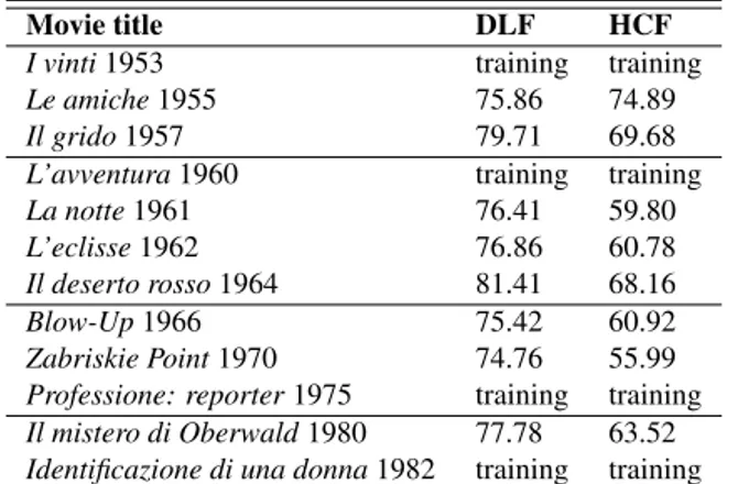
With respect to experiments carried out and presented in [9], we report here an additional test which aims at predicting the shot scale distribution of an entire movie of the Antonioni’s pro-duction, exploring the difference between hand-crafted features (HCF) and deep learnt features (DLF). The idea is to show the ability of the frameworks in generating a robust SSD fingerprint for an unknown movie, where a fingerprint is made up of the three predicted values of CU, MS, and LS percentages, respectively. To this aim we use one Antonioni’s movie per period (i.e. four) to generate the training set (without exploting any a-priori informa-tion on the shot scale distribuinforma-tion), and the remaining eight full movies for testing. We present movie sets and results in terms of accuracy(which measures the proportion of true results) in Table 3. Analysing the results, it seems pretty clear that the CNN ap-proach increases performance in term of accuracy with respect to hand-crafted features.
The ability of both frameworks in estimating the distribution of shot scale in a movie makes possible to extend the study on
(a) (b)
Figure 16. Examples of detected faces (red bounding boxes) a) in a CU and b) in a MS both from Amarcord (1973) directed by Federico Fellini.
(a) (b)
Figure 17. Examples of detected pedestrian (red bounding boxes) a) in a CU and b) in a LS both from Professione: reporter (1975) by Michelangelo Antonioni.
Movie title DLF HCF
I vinti1953 training training
Le amiche1955 75.86 74.89
Il grido1957 79.71 69.68
L’avventura1960 training training
La notte1961 76.41 59.80
L’eclisse1962 76.86 60.78
Il deserto rosso1964 81.41 68.16
Blow-Up1966 75.42 60.92
Zabriskie Point1970 74.76 55.99
Professione: reporter1975 training training Il mistero di Oberwald1980 77.78 63.52 Identificazione di una donna1982 training training Accuracy of prediction of SSD on full Antonioni’s movies us-ing LF (learnt features) and HCF (hand-crafted features). movies from different authors and different ´epoques. Performing a systematic SSD evaluation on a large collection of films from the Internet Movie Database (IMDb) [19] would probably allow to discover patterns of regularity across periods and different di-rectors, thus opening interesting research lines regarding the pos-sible aesthetic and cognitive sources of such regularities.
(a) (b)
Figure 18. Examples of global magnitude of the Fourier transform of a) Long shot (natural scene) and b) a Medium Shot (man-made scene) both taken from L’avventura (1960) by Michelangelo Antonioni (the white plots represent the 80% of the energy).
Mind reading from fMRI
“Mind reading” based on neural decoding is an ambitious line of research within contemporary neuroscience. Assuming that certain psychological processes and mental contents may be encodedin the brain as specific and consistent neural activity pat-terns, researchers in this field aim to decode and reconstruct them given only the neural data. To perform decoding it is necessary to learn a distributed model capable of predicting, based on the associated measurements, a categorical or a continuous label as-sociated with a subject’s perception. The classic approach, often referred to as Multi-Voxel Pattern Analysis (MVPA), uses classi-fication and identifies a discriminating brain pattern that can be used to predict the category of a new, unseen stimuli.
Motivations and aims
Several remarkable neural decoding achievements have been reported so far, mainly in studies employing functional mag-netic resonance imaging (fMRI), but also in intracranial record-ing and electro- and magneto- encephalography experiments (see [41, 42]). These achievements include the successful decoding of mental states such as action intentions [43], reward assessment [44] and response inhibition [45, 46], as well as the reconstruc-tion of various perceptual contents. The latter category contains two types of elements: (i) low-level features, which are physical properties of the stimulus such as light intensity and sound wave patterns; (ii) semantic features, which relate to the psychological meaning attributed to certain clusters of such low-level patterns.
Examples for successful decoding of low-level features in-clude the reconstruction of dynamic video content [47], low-level feature timecourses [48], geometrical patterns, and text [49, 50, 51, 52], and the prediction of optical flow in a video game [53, 54]. Remarkable semantic decoding was gained in the classi-fication of animal categories [55, 56, 57], categorization of com-plex video content in relation to a rich and hierarchical semantic space (including dichotomies such as biological/ non-biological, civilization/ nature [58], semantic classification of visual imagery during sleep [51], and the decoding of types of actions and en-counters (e.g., meeting a dog, observing a weapon) in a video game [53, 54]. This productive stream of research supports the appealing vision of generating a repertoire of “fMRI fingerprints” for a wide range of mental states and perceptual processes (or “cognitive ontology”, see [46]).
When dealing with visual stimuli, the brain community is making more and more use of deep neural networks, for their ca-pability and flexibility in image and video description. On the other hand, neural network researchers have always been inspired by the brain mechanisms while developing new methods. How-ever building an fMRI decoder with the typical structure of Con-volutional Neural Network (CNN), i.e. learning multiple level of representations, seems impractical due to lack of brain data.
As a possible solution, this study presents the first hybrid fMRI and deep features decoder, linking fMRI of movie viewers and video descriptions extracted with deep neural networks [10]. The obtained model is able to reconstruct, using fMRI data, the deep features so that to exploit their discrimination ability. The link is achieved by Canonical Correlation Analysis (CCA) [59] and its kernel version (kCCA), which relates whole-brain fMRI data and video descriptions, finding the projections of these two sets in two new spaces that maximise their linear correlation.
fMRI acquisition and preparation
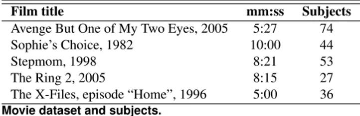
Data consist of ∼230 Voxel Time Course (VTC) scans (∼42000 voxels) taken while watching a total of ∼37 minutes videos from 5 movies, collected from several independent sam-ples of healthy volunteers using a 3 Tesla GE Signa Excite scan-ner. In Table 4 essentials information about movies and subjects are reported (see [10] for more details).
Film title mm:ss Subjects
Avenge But One of My Two Eyes, 2005 5:27 74
Sophie’s Choice, 1982 10:00 44
Stepmom, 1998 8:21 53
The Ring 2, 2005 8:15 27
The X-Files, episode “Home”, 1996 5:00 36 Movie dataset and subjects.
Video object features
Features are extracted and collected from video frames as described in Figure 19 and 20. First each processed frame feeds a
frame faster RCNN object detection
fc7 fc7 argmax conf. num_classes tvmonitor.99 fc7+confidence 1 4096 person.99 person.73 max confidence num_classes fc7 4096 max step
Figure 19. Feature extraction procedure for each processed frame in the video (5fps).
faster R-CNN framework [60]. Multiple objects, together with their related confidence values and last fully connected layer ( f c7), are therefore extracted from each processed frame at dif-ferent scales and aspect ratios. f c7 features are the last fully con-nected layers before classification (softmax) and are considered as highly representative feature of the object class and shape [61]. Since it is possible to have in one frame multiple detections of the same object class (as in Figure 19 for the class “person”), for each class only the f c7 layer of the object with maximum confidence is kept. For this work only “person” class is considered, obtaining a 4096 dimension feature vector from each frame.
The whole procedure is performed at a frame rate of 5 f ps on the entire video. As shown in Figure 20, in order to properly align the f c7 feature matrix with the VTC data resolution (3 s), f c7 fea-ture vectors are averaged on sets of 15 frames. Different subjects and different movies are concatenated along the time dimension, maintaining the correspondence between fMRI and visual stim-uli, so that subjects watching the same movie share the same f c7 features, but different fMRI data.
Linking method
We learned multivariate associations between the VTC from fMRI data and the deep features f c7 using Canonical Correlation Analysis(CCA). Originally introduced by Hotelling [59], CCA aims at transforming the original datasets by linearly projecting them, using matrices A and B, onto new orthogonal matrices U and V whose columns are maximally correlated: the first compo-nent (column) of U is highly correlated with the first of V , the second of U with the second of V , and so on.
00:00 00:01 00:02 00:03 00:04 00:05 00:06 time [mm:ss] ... 1 5 10 15 20 25 30 ... [frame] fMRI VTC mean on 3[s] reshape concatenation fc7 fMRI reshape t_samples num_voxels and Z-score concatenation and Z-score t_samples 4096 ... ...
Figure 20. Extraction and normalization of f c7 features from the video stream (top) and volume time courses (VTC) extraction from fMRI data (bot-tom) for one movie and one subject. New subjects and movies are concate-nated in time dimension.
During training (Fig. 21-a), matrices U and V are obtained from VTC data and f c7 features. The correlation between U and V components is validated using new data (different sub-jects and/or movies) to assess its robustness. In the testing step (Fig. 21-b), the decoding procedure is performed starting from VTC data and obtaining f c7 through the matrices A and B previ-ously found. We show how this scheme can be used to perform a classification task based on the reconstructed f c7 matrix.
fMRI reshape A+ (t_samples, 4096) fc7 VTC (4096, numCC) A B V U
(t_samples, num_voxels) (num_voxels, numCC) (t_samples, numCC)
Multiplication order Multiplication order
T T T T (1, 4096) fc7 VTC (numCC, 4096) B V U
(1, num_voxels) (num_voxels, numCC) (1, numCC)
Multiplication order Multiplication order
+ (a) Training: V = V TC × B, U = f c7 × A
fc
7
⌢ˆ
fMRI reshape A+ (t_samples, 4096) fc7 VTC (4096, numCC) A B V U(t_samples, num_voxels) (num_voxels, numCC) (t_samples, numCC)
Multiplication order Multiplication order
T T T T (1, 4096) fc7 VTC (numCC, 4096) B V U
(1, num_voxels) (num_voxels, numCC) (1, numCC)
Multiplication order Multiplication order
+
(b) Testing: V = V TC × B, f c7 = U × A+
Figure 21. Mapping procedure between video object features ( f c7) and brain data (VTC) in (a) training (single step) and (b) testing (repeated for every time point). Some matrices are transposed in the figure for display purposes: please refer to formulas and displayed matrix dimensions.
When the number of time samples is lower than data dimen-sion (i.e. voxels number), the estimation of the canonical compo-nents is ill-posed. We therefore used a variant with a linear kernel in combination with a quadratic penalty term (L2-norm), to esti-mate A and B, using the Python module Pyrcca [62]. In addition we account for the haemodynamic effects in the fMRI signal by introducing a shift between the two datasets.
Experiments
After parameter tuning (see [10] for details), we first gen-eralize the model to new subjects and/or movies, and then show classification performance on an exemplary discrimination task.
Generalization to new subjects and movies
With λ = 10−2 and a time shift of two samples, we esti-mated a kCCA model using the 35 training subjects of the movie Sophie’s Choice. Figure 22-a shows the correlations between the first 10 canonical components on the training and on the left-out, testing dataset (9 subjects). Training and testing features are per-muted scrambling the phase of the Fourier transform with respect to the original ones, repeating the entire training-testing procedure 300 times on randomly permuted features.
We further explored the robustness of the method by gen-eralizing this model on the remaining movies. Significance was determined with the phase scrambling permutation process only on testing movies (500 times), leaving unchanged the training set (Sophie’s Choice). The results are shown in Figure 22-b; in this case, three movies (The Ring 2, Stepmom and The X-Files) show significant correlations among the first ten components. However
* p=0.003 * * * * * * * * * *
(a) Single movie
* p<0.05, ** p<0.01, *** p<0.005 *** *** ** *** *** *** *** *** *** *** *** *** *** *** *** *** *** *** *** *** *** * *** (b) Across movies
Figure 22. a) Correlation on a single movie (Sophie’s Choice) on all test subjects (similar values on all movies); b) correlation results across movies and across subjects (training on Sophie’s Choice).
the movie Avenge does not: one possible explanation for this be-haviour can be found in the different stylistic choices adopted by directors in the five movies, for example in the use of the shot scale, light conditions or video motion. Even if previous correla-tion results obtained on single movies are good indicators about the soundness of the proposed approach, this stylistic interpreta-tion has to be fully proven in later stages of the work.
Classification
As a last experiment we show how the linking between deep neural networks and brain data can be beneficial to subtle classi-fication tasks. Since in this work we consider only the f c7 fea-tures related to the class person, we chose, as an example, to
dis-(a) Accuracy (b) F1 measure
Figure 23. Classification performance comparison between: f c7 features only (blue), fMRI data only (red), and our method for predicting f c7 features from fMRI data across subjects. Performance are shown in terms of a) Ac-curacy and b) F1-measure. Shading describes standard deviation across subjects.
criminate the portion of human figure shot in the video frames, distinguishing between two classes: face only (face) or full fig-ure (pedestrian) by conducting three analyses. Face and pedes-trian ground truth is manually annotated for every time repetition (TR=3s). All analyses involve a single movie Sophie’s Choice, selecting the 35 training VTCs and the 9 testing VTCs as before.
First, we evaluated classification using whole-brain fMRI data only; a linear SVM classifier was trained using balanced (across classes) training samples selected from the 35 training VTCs and tested on the 9 testing VTCs. Given the large dimen-sions of the fMRI data, the relatively fine-grained difference be-tween the two classes, and the individual differences across sub-jects, poor performance are expected. Second, we classified using f c7 features; this could be considered as an upper bound: since these features are inherently capable of discriminating different shapes, excellent results are expected. The f c7 features were ran-domly split into training and testing (75%-25%), and a balanced SVM classifier with linear kernel was trained and tested. Last, we used the proposed link between f c7 and VTC and reconstructed the deep neural network features starting from the observed test fMRI data. Given a VTC with 1 TR, we follow the pipeline shown in Figure 21-b obtaining a f c7-like vector. f c7 were re-constructed from V using the Moore-Penrose pseudo-inverse of A. We finally learned a balanced linear SVM with 35 training VTCs and testing with the remaining 9. Different number of canonical components numCC were considered.
All results (fMRI only, f c7 predicted from fMRI, and f c7 only) are presented in Figure 23, in terms of a) accuracy and b) F1-measure. As we expected, our method significantly improves the classification performance with respect to the classifier trained with fMRI data only, both in terms of accuracy (up to 55%) and F1-measure (up to 80%). Best performance are obtained with 10 components, which is a sufficiently large number to exploit the discriminative properties of f c7 features, but small enough to keep good classification performance. Results also show a low variability across different subjects, thus underling once again the ability of the proposed method to generalize well across subjects. Preliminary results shown in this empirical study demon-strate the ability of the method to effectively embed the imaging data onto a subspace more directly related to the classification task at hand. To facilitate fine-grained classification tasks, we need in the future to extend this approach to other object classes (car, house, dog, etc.) and test it on other movies.
Conclusion
Because of the illusion of reality they provide, cinema movies have become in the last half century one of the preferred testbeds addressed by scientific studies. Computer Vision meth-ods, either based on hand-crafted or deep learnt features, offer a valuable set of techniques to obtain movie content representations useful to approach very different research questions.
Aiming at providing affective based recommendation, we explore the connotative meaning of movies: the set of stylis-tic conventions filmmakers use very consciously to persuade, in-spire, or soothe the audience. Without the need of registering user’s physiological signals neither by employing people emo-tional rates, but just relying on the inter-subjectivity of conno-tative concepts and on the knowledge of user’s reactions to sim-ilar stimuli, connotation provides an intermediate representation which exploits the objectivity of audiovisual descriptors to sug-gest filmic content able to target users’ affective requests.
A key mental process that channels the impact of audio-visual narratives on audiences is empathy, defined as the under-standing and experiencing mental states of an observed other per-son. Among audio-visual features, the shot scale greatly influ-ences the empathy response of the audience. We therefore pro-pose two frameworks for performing a second-based measure-ment of shot scale in movies. As a result the shot scale distri-bution, beyond playing an important role in the film’s emotional effect on the viewer, might be as well an important authorial fin-gerprint to be further explored in a systematic manner.
Remarkable achievements have been recently made in the reconstruction of audiovisual and semantic content by means of decoding of neuroimaging data. Inspired by the revolution we are witnessing in the use of deep neural networks, we first approached the problem of decoding deep features starting from fMRI data. Excellent results in terms of correlation are obtained across dif-ferent subjects and good results across difdif-ferent movies. Future efforts will be spent in several directions, among which broaden-ing the analysis to other classes (car, house, dog, etc.) and other movies.
References
[1] M. Az´ema and F. Rivere, Animation in palaeolithic art: a pre-echo of cinema, Antiquity, vol. 86, no. 332, pg. 316–324, 006 (2012). [2] B.A. V¨ollm, A.N.W. Taylor, P. Richardson, R. Corcoran, J. Stirling,
S. McKie, J.F.W. Deakin, and R. Elliott, Neuronal correlates of the-ory of mind and empathy: A functional magnetic resonance imaging study in a nonverbal task, NeuroImage, vol. 29, no. 1, pg. 90 – 98 (2006).
[3] H.L. Gallagher and C.D. Frith, Functional imaging of ’theory of mind’, Trends in Cognitive Sciences, vol. 7, no. 2, pg. 77 – 83 (2003).
[4] P.G. Blasco and G. Moreto, Teaching empathy through movies: Reaching learners’ affective domain in medical education, Journal of Education and Learning, vol. 1, no. 1, pg. 22 (2012).
[5] Y. LeCun, L. Bottou, Y. Bengio, and P. Haffner, Gradient-based learning applied to document recognition, Proceedings of the IEEE, vol. 86, no. 11, pg. 2278–2324 (1998).
[6] T. Naselaris, K.N. Kay, S. Nishimoto, and J.L. Gallant, Encoding and decoding in fMRI, NeuroImage, vol. 56, no. 2, pg. 400 – 410 (2011).
[7] S. Benini, L. Canini, and R. Leonardi, A connotative space for
supporting movie affective recommendation, IEEE Transactions on Multimedia, vol. 13, no. 6, pg. 1356–1370 (2011).
[8] L. Canini, S. Benini, and R. Leonardi, Affective recommendation of movies based on selected connotative features, Circuits and Systems for Video Technology, IEEE Transactions on, vol. 23, no. 4, pg. 636– 647 (2013).
[9] S. Benini, M. Svanera, N. Adami, R. Leonardi, and A.B. Kov´acs, Shot scale distribution in art films, Multimedia Tools and Applica-tions, vol. 75, no. 23, pg. 16499–16527 (2016).
[10] M. Svanera, S. Benini, G. Raz, T. Hendler, R. Goebel, and G. Va-lente, Deep driven fmri decoding of visual categories, in NIPS Work-shop on Representation Learning in Artificial and Biological Neural Networks (MLINI 2016), Barcelona, Spain, December 9(2016). [11] V. Gallese and M. Guerra, Lo schermo empatico: cinema e
neuro-scienze, R. Cortina, 2015.
[12] E. S. H. Tan, Film-induced affect as a witness emotion, Poetics, vol. 23, no. 1, pg. 7–32, (1995).
[13] G. M. Smith, Film Structure and the Emotion System, Cambridge University Press, Cambridge, 2003.
[14] D. Arijon, Grammar of the Film Language, Silman-James Press, 1991.
[15] R. M. Weaver, A Rhetoric and Composition Handbook, William Morrow & Co., New York, NY, 1974.
[16] C. T. Castelli, Trini diagram: imaging emotional identity 3d posi-tioning tool, The International Society for Optical Engineering, vol. 3964, pg. 224–233, December (1999).
[17] C. Osgood, G. Suci, and P. Tannenbaum, The Measurement of Meaning, University of Illinois Press, Urbana, IL, 1957.
[18] What is a Great Film Scene or Great Film Moment? An introduction to the topic, http://www.filmsite.org/scenes.html, [Online; accessed 8-November-2016].
[19] IMDb, Internet movie database, 2016, [Online; accessed 8-November-2016].
[20] P.E. Shrout and J.L. Fleiss, Intraclass correlations: Uses in assessing rater reliability, Psychological Bulletin, vol. 86, no. 2, pg. 420–428 (1979).
[21] M. Kendall and J. D. Gibbons, Rank Correlation Methods, Edward Arnold, 1990.
[22] Y. Rubner, C. Tomasi, and L. Guibas, The earth mover’s distance as a metric for image retrieval, International Journal of Computer Vision, vol. 40, no. 2 (2000).
[23] H. Peng, F. Long, and C. Ding, Feature selection based on mutual information: criteria of max-dependency, max-relevance, and min-redundancy, IEEE Transactions on Pattern Analysis and Machine Intelligence, vol. 27, no. 8 (2005).
[24] A.B. Kov´acs, Shot scale distribution: an authorial fingerprint or a cognitive pattern?, Projections, vol. 8, no. 2 (2014).
[25] M. Svanera, S. Benini, N. Adami, R. Leonardi, and A. B. Kov´acs, Over-the-shoulder shot detection in art films, in 13th International Workshop on Content-Based Multimedia Indexing, CBMI 2015, Prague, Czech Republic, June 10-12, 2015, pg. 1–6, IEEE (2015). [26] B. Bal´azs, Der sichtbare Mensch, Berlin, 1924.
[27] L. Canini, S. Benini, and R. Leonardi, Affective analysis on pat-terns of shot types in movies, in Image and Signal Processing and Analysis (ISPA), 2011 7th International Symposium on. IEEE, 4-6 September 2011, pg. 253–258 (2011).
[28] X. Cao, The effects of facial close-ups and viewers’ sex on empathy and intentions to help people in need, Mass Communication and Society, vol. 16, no. 2, pg. 161–178 (2013).
[29] D. Mutz, Effects of ’in-your-face’ television discourse on percep-tions of a legitimate opposition, American Political Science Review, vol. 101, no. 4, pg. 621–635, 11 (2007).
[30] K. B´alint, T. Klausch, and T. P´olya, Watching closely, Journal of Media Psychology, vol. 0, no. 0, pg. 1–10 (2016).
[31] B. Bal´azs and E. Carter, B´ela Bal´azs: Early film theory: Visible man and the spirit of film, vol. 10, Berghahn Books, 2010.
[32] N. Carroll, Toward a theory of point-of-view editing: Communi-cation, emotion, and the movies, Poetics Today, vol. 14, no. 1, pg. 123–141 (1993).
[33] P. Persson, Understanding cinema: A psychological theory of mov-ing imagery, Cambridge University Press, 2003.
[34] C. Plantinga, The scene of empathy and the human face on film, Pas-sionate views: Film, cognition, and emotion, pg. 239–255, (1999). [35] M. Smith, Engaging characters: Fiction, emotion, and the cinema,
Clarendon Press Oxford, 1995.
[36] Wikipedia, Art film — wikipedia, the free encyclopedia, 2015, [On-line; accessed 20-March-2015].
[37] C. Cortes and V. Vapnik, Support-vector networks, Machine learn-ing, vol. 20, no. 3, pg. 273–297 (1995).
[38] L. Breiman, Random forests, Machine learning, vol. 45, no. 1, pg. 5–32 (2001).
[39] A. Krizhevsky, I. Sutskever, and G.E. Hinton, Imagenet classifica-tion with deep convoluclassifica-tional neural networks, in Advances in Neural Information Processing Systems 25, pg. 1097–1105. Curran Asso-ciates, Inc. (2012).
[40] O. Russakovsky, J. Deng, H. Su, J. Krause, S. Satheesh, S. Ma, Z. Huang, A. Karpathy, A. Khosla, M. Bernstein, A.C. Berg, and L. Fei-Fei, Imagenet large scale visual recognition challenge, Inter-national Journal of Computer Vision, vol. 115, no. 3, pg. 211–252 (2015).
[41] M. Chen, J. Han, X. Hu, X. Jiang, L. Guo, and T. Liu, Survey of encoding and decoding of visual stimulus via fmri: an image analy-sis perspective, Brain Imaging and Behavior, vol. 8, no. 1, pg. 7–23 (2014).
[42] J.V. Haxby, Multivariate pattern analysis of fmri: the early begin-nings, Neuroimage, vol. 62, no. 2, pg. 852–855 (2012).
[43] J.D. Haynes, K. Sakai, G. Rees, S. Gilbert, C. Frith, and R.E. Pass-ingham, Reading hidden intentions in the human brain, Current Biology, vol. 17, no. 4, pg. 323 – 328 (2007).
[44] T. Kahnt, J. Heinzle, S.Q. Park, and J.D. Haynes, Decoding dif-ferent roles for vmpfc and dlpfc in multi-attribute decision making, NeuroImage, vol. 56, no. 2, pg. 709 – 715 (2011),
[45] J.R. Cohen, R.F. Asarnow, F.W. Sabb, R.M. Bilder, S.Y. Bookheimer, B.J. Knowlton, and R.A. Poldrack, Decoding develop-mental differences and individual variability in response inhibition through predictive analyses across individuals, Frontiers in Human Neuroscience, vol. 4, pg. 47 (2010).
[46] R.A. Poldrack, Y.O. Halchenko, and S.J. Hanson, Decoding the large-scale structure of brain function by classifying mental states across individuals, Psychological Science, vol. 20, no. 11, pg. 1364– 1372 (2009).
[47] S. Nishimoto, A.T. Vu, T. Naselaris, Y. Benjamini, B. Yu, and J.L. Gallant, Reconstructing visual experiences from brain activ-ity evoked by natural movies, Current Biology, vol. 21, no. 19, pg. 1641 – 1646 (2011).
[48] G. Raz, M. Svanera, G. Gilam, M. B. Cohen, T. Lin, R. Admon, T. Gonen, A. Thaler, R. Goebel, S. Benini, and G. Valente, Ro-bust inter-subject audiovisual decoding in fMRI using kernel ridge
regression, (to be submitted to) Nature Methods (2017).
[49] Y. Fujiwara, Y. Miyawaki, and Y. Kamitani, Estimating image bases for visual image reconstruction from human brain activity, in Advances in neural information processing systems, pg. 576–584 (2009).
[50] Y. Miyawaki, H. Uchida, O. Yamashita, M. Sato, Y. Morito, H.C. Tanabe, N. Sadato, and Y. Kamitani, Visual image reconstruction from human brain activity using a combination of multiscale local image decoders, Neuron, vol. 60, no. 5, pg. 915 – 929 (2008). [51] M.A.J. Van Gerven, F.P. De Lange, and T. Heskes, Neural decoding
with hierarchical generative models, Neural computation, vol. 22, no. 12, pg. 3127–3142 (2010).
[52] K. Yamada, Y. Miyawaki, and Y. Kamitani, Inter-subject neural code converter for visual image representation, NeuroImage, vol. 113, pg. 289–297 (2015).
[53] C. Chu, Y. Ni, G. Tan, C.J. Saunders, and J. Ashburner, Kernel regression for fmri pattern prediction, NeuroImage, vol. 56, no. 2, pg. 662 – 673 (2011).
[54] G. Valente, F. De Martino, F. Esposito, R. Goebel, and E. Formisano, Predicting subject-driven actions and sensory experience in a vir-tual world with Relevance Vector Machine Regression of fMRI data, NeuroImage, vol. 56, no. 2, pg. 651–661, May (2011).
[55] A.C. Connolly, J.S. Guntupalli, J. Gors, M. Hanke, Y.O. Halchenko, Y.-C. Wu, H. Abdi, and J.V. Haxby, The representation of biological classes in the human brain, Journal of Neuroscience, vol. 32, no. 8, pg. 2608–2618 (2012).
[56] J.V. Haxby, J.S. Guntupalli, A.C. Connolly, Y.O. Halchenko, B.R. Conroy, M.I. Gobbini, M. Hanke, and P.J. Ramadge, A common, high-dimensional model of the representational space in human ven-tral temporal cortex, Neuron, vol. 72, no. 2, pg. 404 – 416 (2011). [57] J.V. Haxby, M.I. Gobbini, M.L. Furey, A. Ishai, J.L. Schouten, and
P. Pietrini, Distributed and overlapping representations of faces and objects in ventral temporal cortex, Science, vol. 293, no. 5539, pg. 2425–2430 (2001).
[58] A.G. Huth, S. Nishimoto, A.T. Vu, and J.L. Gallant, A continuous semantic space describes the representation of thousands of object and action categories across the human brain, Neuron, vol. 76, no. 6, pg. 1210 – 1224 (2012).
[59] H. Hotelling, Relations between two sets of variates, Biometrika, vol. 28, no. 3/4, pg. 321–377 (1936).
[60] S. Ren, K. He, R. Girshick, and J. Sun, Faster R-CNN: Towards real-time object detection with region proposal networks, in Advances in Neural Information Processing Systems, pg. 91–99 (2015). [61] J. Donahue, Y. Jia, O. Vinyals, J. Hoffman, N. Zhang, E. Tzeng, and
T. Darrell, DeCAF: A Deep Convolutional Activation Feature for Generic Visual Recognition, Icml, vol. 32, pg. 647–655 (2014). [62] N.Y. Bilenko and J.L. Gallant, Pyrcca: regularized kernel canonical
correlation analysis in python and its applications to neuroimaging, arXiv preprint arXiv:1503.01538(2015).
Author Biography
Sergio Benini received his MSc degree in Electronic Engineering (2000, cum laude) and his PhD in Information Engineering (2006) from the University of Brescia, Italy. Between 2001 and 2003 he was with Siemens Mobile Communications R&D. During his Ph.D. he spent almost one year in British Telecom Research in UK. Since 2005 he is Assistant Professor at the University of Brescia. In 2012 he co-founded Yonder http: // yonderlabs. com , a spin-off company specialized in NLP, Ma-chine Learning, and Cognitive Computing.