DOTTORATO DI RICERCA IN
INGEGNERIA CIVILE E AMBIENTALE
Curriculum: Analisi e gestione dei rischi naturali
Settore Scientifico Disciplinare: ICAR/02 Costruzioni idrauliche e marittime e Idrologia
XXXI CICLO
Sediment yield and transport:
estimation and climate influence
Relatore e Tutor:
Tesi di Dottorato di:
Prof. Giovanna Grossi
Francesca Berteni
Coordinatore del Dottorato:
Prof. Paolo Secchi
Abstract
Erosion, transfer and deposition of soil particles due to water and the impact of climate change on these physical processes have acquired a great importance during the last decades. Indeed, it is the subject of focused research in several fields of the earth sciences (such as hydrology, hydraulics, ecology, agriculture, geology, civil and environmental engineering, etc.), as the result of the continuous increase in hydrogeological risk in different geographical areas around the world, including Italy. Knowledge of the sediment volumes generated and transported by streams is useful, for example, for the successful design of hydraulic infrastructures, dams or reservoirs, for changes to forest waterways and terrain, for the land management and environment, etc.
Sediment production at the catchment scale and solid transport in rivers can be assessed and quantified through mathematical and empirical models. Unfortunately, there is a shortage of gauged data regarding sediment fluxes and production at the catchment scale, because of topographical and pedological complexity and high spatial variability of all the hydrological characteristics. Another point that should be taken into account is the scarce availability of the appropriate equipment to make survey measurements. For these reasons, it is hard to implement monitoring techniques. However, in the absence of field data, major elements for land management, planning and protection include an estimate of soil loss and sediment yield and their comparison with other case studies.
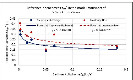
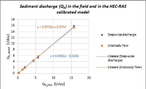
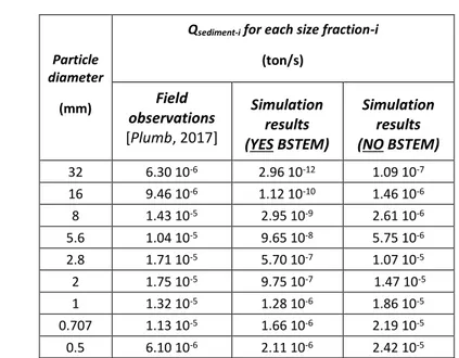
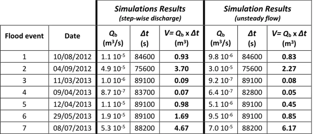
In the first part of this thesis project, a detailed sediment transport analysis in a reach of the Mimico Creek, which is located in Southern Ontario (Canada), was conducted by making use of the sediment transport investigations. A hydraulic model was developed and calibrated through the HEC-RAS software, by using the Wilcock and Crowe transport function, to a series of discharge events where in-situ bedload sampling occurred. Bedload samplings used in calibrating the transport model were limited by the orifice of the Helley-Smith bedload sampler (ranging between 0.5 mm and 32 mm). Calibration curves, that determine bed material transport rates as a function of the dimensionless reference shear stress, were created considering both step-wise discharge and unsteady flow simulations. The results of the calibrated model were used to calculate the mean travel distance of bed material: the goal was to compare the simulation results achieved to field observations, derived through the bed material particle tracking (RFID technique). The values achieved showed that the Wilcock and Crowe equation under-predicts the transport of the coarsest fractions in the bed load and that the travel distances calculated considering the BSTEM option (which also considers the presence of fine material from bank erosion) are longer. Finally, the travel distances of different grain sizes were estimated using the calibrated model results. The obtained values showed that particles have a steep reduction in travel distance with an increase in their size. Furthermore, transport distance values are higher for the flood events with higher peak discharges, generally in accordance with field measurements. The fractional transport distances of different grain classes estimated by using simulation results
while when using simulation results, both mobile and immobile particles were taken into account.
In the second part of this thesis project, a mean annual estimation of soil loss due to water erosion in the Guerna catchment, which is located in the Province of Bergamo (Northern Italy), was made in a GIS environment. Soil loss was estimated using the RUSLE and EPM models. Results showed that the mean annual value of soil loss computed through the RUSLE equation (302271 t/year) is about three times higher than its evaluation according to the EPM method (302634 m3/year, which corresponds to 83225 t/year by considering a specific
weight of 2.75 t/m3). This estimate is coherent with the values obtained for other case
studies and, in line with them, it can be said that the EPM approach is more suitable to water erosion assessment in mountain catchments. These estimations of mean annual value soil loss were evaluated also considering a spatial analysis of soil erosion trends in three different future climate scenarios, in line with the last IPCC Assessment Report. Results showed that, applying the RUSLE equation to different climate change scenarios, there are no relevant soil loss increases. The soil loss calculated using the EPM method for two of the three future scenarios is larger than the value estimated without considering climate change. Only rainfall and temperature regimes were considered to evaluate the effects of climate change on water erosion; the future variations of the land use were reasonably omitted. According to the EPM method and to the future scenarios, the annual average soil loss could change by 8-10% on a basin scale. Finally, the sediment yield for an analysed rainfall event was also estimated in the Guerna catchment, in order to create a combined sediment yield and solid transport system. Sediment yield was estimated in the Guerna catchment using the MUSLE equation in a GIS environment and the mean value achieved (32.5 t∙ha-1) is approximately
one-third of the soil loss mean annual value obtained by the RUSLE model (97.7 t∙ha-1∙year -1). The sediment yield for the rainfall event analysed was also estimated, using the MUSLE
equation, for the 7 sub-basins identified in the Guerna catchment. The found values were used as input sediment load in the HEC-RAS model, that was developed for the Guerna Creek in order to simulate sediment transport. Wilcock and Crowe is the transport function that was chosen and the “Time-Area method” was adopted to create runoff hydrographs. The mean value of sediment discharge achieved is 6632 t/d and 66810 t/d, respectively at the upstream cross section and downstream cross section of the study reach. The downstream cross section is the Guerna watershed outlet, with an area of 30.9 km2. The upstream cross
section is the outlet of its upstream sub-basin, with an area of 3 km2. Results are comparable
to the measured value in the Rio Cordon catchment, a small mountain basin (5 km2) in the
northeastern Italian Alps with similar characteristics to the Guerna catchment: during an intensive flood event the sediment discharge recorded is 8040 t/d.
Keywords: water erosion, soil loss, sediment yield, climate change, RUSLE, EPM, MUSLE,
Sommario
L’erosione, il trasporto e il deposito di particelle solide dovuti all’azione dell’acqua e l’impatto del cambiamento climatico su questo fenomeno fisico ha acquisito grande importanza, in particolare durante gli ultimi decenni. Infatti è oggetto di ricerca in molti campi legati alle scienze della terra (ad esempio l’idrologia, l’idraulica, l’ecologia, le scienze agrarie, la geologia, l’ingegneria civile e ambientale, ecc.) a causa di un continuo aumento del rischio idrogeologico in diverse aree geografiche del mondo, non esclusa l’Italia. Conoscere il volume di sedimenti prodotti dall’erosione idrica e trasportati dai corpi idrici è utile, ad esempio, per la corretta progettazione di infrastrutture idrauliche, dighe o serbatoi di accumulo, per interventi di sistemazione idraulico-forestale, per la gestione del territorio e dell’ambiente, ecc.
La produzione di sedimenti a scala di versante e il trasporto solido nei fiumi possono essere valutati e quantificati servendosi di modelli matematici ed empirici. Purtroppo le misure di campo relativamente alla produzione e al trasporto di sedimenti a scala di bacino sono molto scarse e difficilmente applicabili in contesti geomorfologici diversi, a causa sia della complessità topografica e pedologica sia dell’alta variabilità spaziale delle caratteristiche idrologiche. Un altro elemento da tenere in considerazione è l’effettiva, spesso scarsa, disponibilità di una strumentazione adeguata per effettuare misure di campo. A fronte di queste ragioni, risulta difficile applicare tecniche di monitoraggio. Tuttavia, in assenza di dati di campo, una stima dell’ordine di grandezza della perdita di suolo e della produzione di sedimenti da confrontare con altri casi studio, sono elementi di non secondaria importanza nella pianificazione della gestione e protezione del territorio.
Nella prima parte del presente lavoro di tesi è stato svolto un accurato studio del trasporto solido su un tratto del torrente Mimico, sito nel sud del Canada (Ontario), servendosi dei dati di campo di portata solida disponibili. È stato costruito e calibrato un modello idraulico tramite il software HEC-RAS, calcolando la portata solida tramite la funzione di trasporto di Wilcock and Crowe e considerando una serie di eventi di piena durante i quali fosse stata effettuata la misura della portata solida. I campioni di terreno adoperati per la calibrazione avevano dimensione granulometrica limitata (da 0.5 mm a 32 mm) a causa delle caratteristiche del campionatore Helley-Smith usato. Le curve di calibrazione, che esprimono la portata solida in funzione dello sforzo tangenziale adimensionale di riferimento, sono state costruite considerando sia il regime di moto quasi-vario sia quello di moto vario. I risultati del modello calibrato sono stati utilizzati per calcolare la distanza media percorsa dal materiale solido di fondo alveo: l’obiettivo era quello di confrontare i risultati ottenuti dall’applicazione del modello con quelli di campo, ricavati grazie alla tecnica RFID. I valori ai quali si è pervenuti hanno mostrato che l’equazione di Wilcock and Crowe sottostima il trasporto delle particelle più grossolane e che, a causa della presenza di materiale a granulometria più fine, le distanze calcolate sono maggiori usando l’opzione BSTEM (che
calcolare le distanze medie percorse dalle singole granulometrie del materiale che costituisce il fondo dell’alveo. I risultati hanno evidenziato una grossa riduzione della distanza percorsa dalle particelle con l’aumentare della loro dimensione. Inoltre, le distanze calcolate risultano maggiori per eventi di piena caratterizzati da un alto valore della portata di picco; quest’ultima considerazione è, in linea generale, in accordo con le misure di campo. Le distanze medie percorse dalle singole granulometrie che sono state calcolate partendo dai risultati della simulazione e che includono sia le particelle mobili che quelle immobili, risultano minori rispetto a quelle misurate in campo, dove vengono prese in considerazione solamente le particelle mobili.
Nella seconda parte del lavoro è stata analizzata in ambiente GIS la perdita di suolo media annua dovuta all’erosione idrica di versante del bacino del torrente Guerna, che ricade nella provincia di Bergamo (Nord Italia). La perdita di suolo è stata stimata utilizzando i modelli RUSLE e EPM. Dai risultati è emerso che il valore medio annuo di perdita di suolo calcolato con l’equazione RUSLE (302271 t/anno) è circa tre volte maggiore rispetto a quello ricavato con col metodo EPM (302634 m3/anno che, considerando un peso specifico pari a 2.75 t/m3,
corrispondono a 83225 t/anno). Questa stima è coerente coi risultati di altri casi studio e, in accordo con questi ultimi, si può affermare che l’approccio EPM sia più adatto ad una valutazione dell’erosione idrica in bacini montani. La perdita di suolo media annua così stimata, è stata valutata considerando anche la variabilità spaziale dell’erosione idrica in tre diversi scenari climatici futuri costruiti in accordo con l’ultimo Rapporto IPCC. I risultati hanno mostrato che, applicando l’equazione RUSLE ai differenti scenari di cambiamento climatico, non si verificano grossi aumenti nella produzione di sedimenti. La perdita di suolo calcolata col metodo EPM risulta maggiore per due dei tre scenari futuri, rispetto al calcolo effettuato senza considerare l’impatto del cambiamento climatico. Solamente il regime di precipitazione e di temperatura sono stati presi in esame per valutare gli effetti del cambiamento climatico sull’erosione idrica; le possibili variazioni future dell’uso del suolo sono state ragionevolmente trascurate. Dall’applicazione del metodo EPM, considerando anche gli scenari futuri, è emerso che la perdita media annua di suolo può variare dal 8% al 10% a scala di bacino. Infine, è stata effettuata una stima della produzione di sedimenti che possono raggiungere la sezione di chiusura del bacino del Guerna, a seguito di un preciso evento meteorico che è stato studiato. L’obiettivo era quello di creare un sistema combinato di erosione idrica e trasporto solido nel torrente Guerna. Il quantitativo di sedimenti che può arrivare alla sezione di chiusura del bacino, in occasione dell’evento meteorico considerato, è stato stimato servendosi del modello MUSLE in ambiente GIS; il valore medio ottenuto (32.5 t∙ha-1) è circa pari ad un terzo della perdita di suolo media annua calcolata col metodo
RUSLE (97.7 t∙ha-1∙anno-1). L’equazione MUSLE è stata applicata anche a 7 sottobacini del
torrente Guerna, per stabilire così la quantità di sedimenti che può raggiungere ciascuna sezione di chiusura dei sottobacini. I valori ottenuti sono stati adoperati come carico di sedimenti in ingresso nel modello HEC-RAS che è stato realizzato per il torrente Guerna, con lo scopo di simulare il suo trasporto solido. La funzione di trasporto che è stata scelta è quella di Wilcock and Crowe e gli idrogrammi in ingresso al modello sono stati costruiti usando il metodo della corrivazione. La portata solida media ottenuta è pari a 6632 t/d e 66810 t/d in corrispondenza, rispettivamente, della sezione a monte e di quella a valle del tratto di
torrente analizzato. La sezione di valle è quella di chiusura del bacino del torrente Guerna con area pari a 30.9 km2, mentre quella di monte è la sezione di chiusura del suo sottobacino
di monte con area di 3 km2. I risultati ai quali si è pervenuti sono paragonabili con quelli
misurati in campo, in occasione di un importante evento di piena, nel bacino di 5 km2 del Rio
Cordon (8041 t/d), sito nell’Italia nord-orientale (Veneto) e avente caratteristiche simili.
Parole-chiave: erosione idrica, perdita di suolo, produzione di sedimenti che raggiungono la
Index
1. Introduction ... 11
1.1. Background and goals... 13
1.2. Outline of the document ... 14
1.3. Acknowledgments ... 15
1.4. Acronyms ... 16
2. Transport of sediments in rivers ... 19
2.1. Introduction ... 21
2.2. Sediment transport process and initiation of motion ... 22
2.3. Sediment transport modelling ... 25
2.3.1. Sediment transport functions ... 25
2.3.2. Sediment transport functions calibration ... 30
2.4. Virtual rate of travel and mean bed material travel distances ... 30
2.5. Sediment transport in rivers: case study examples ... 32
3. The Mimico Creek case study ... 39
3.1. Introduction and goals ... 41
3.2. Catchment characteristics ... 42
3.3. July 8th, 2013: extreme rainfall event ... 46
3.4. Sediment transport measurements and flow hydrographs ... 49
3.5. Construction of the HEC-RAS model... 57
3.5.1. Geometry data ... 57
3.5.2. Sediment Data ... 58
3.5.2.1. Sensitivity analysis: the effects of the BSTEM ... 61
3.5.3. Flow Data ... 61
3.6. Flood wave propagation in unsteady flow ... 63
3.7. Changes in water levels and tides ... 66
3.8.3. Comparison between calibration with and without the BSTEM ... 71
3.9. Mean travel distance of bed material using HEC-RAS results ... 74
3.9.1. Mean travel distance considering the BSTEM ... 75
3.9.2. Mean travel distance without considering the BSTEM ... 77
3.9.3. Comparison between mean travel distances estimated by considering and without considering the BSTEM ... 79
3.10. Mean travel distance of different grain sizes of bed material using HEC-RAS results ... 80
3.11. Concluding remarks ... 84
4. Water erosion and climate change... 87
4.1. Introduction ... 89
4.2. Water erosion, transfer and deposition processes ... 90
4.3. Mathematical sediment models ... 92
4.3.1. Empirical sediment models ... 94
4.3.1.1. RUSLE model ... 94
4.3.1.2. MUSLE model... 100
4.3.1.3. EPM model ... 100
4.4. Water erosion: case study examples ... 101
4.5. Impact of climate change ... 106
4.5.1. CORDEX experiment ... 106
5. The Guerna catchment case study ... 109
5.1. Introduction and goals ... 111
5.2. Catchment characteristics ... 112
5.2.1. Location and thematic maps ... 112
5.2.2. Hypsographic and hypsometric curve ... 115
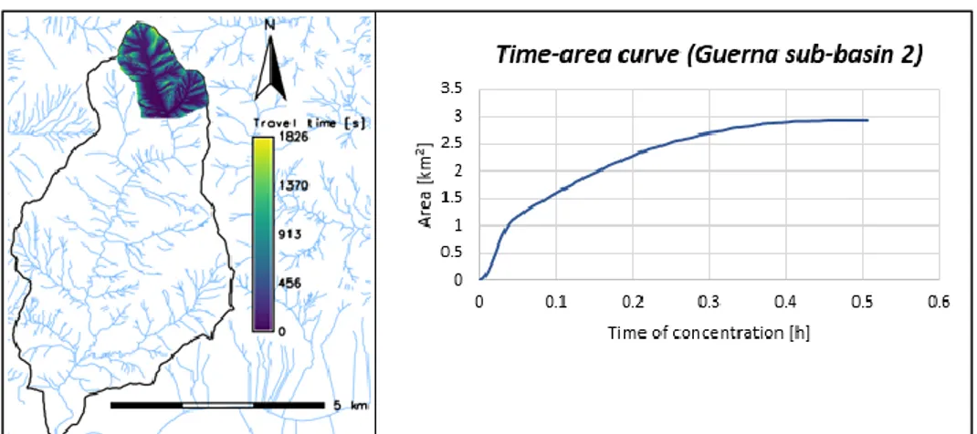
5.2.3. Time of concentration and time-area function ... 118
5.3. Application of the RUSLE model ... 126
5.3.1. Comparison with the European Soil Data Centre (ESDAC) ... 130
5.4. Application of the EPM method ... 134
5.5. Application of the RUSLE model considering the impact of climate change ... 140
5.7. The effect of climate change on land use ... 153
5.8. Application of the MUSLE model ... 156
5.8.1. Guerna catchment ... 156
5.8.2. Sub-basins identified in the Guerna catchment ... 161
5.9. The HEC-RAS model ... 165
5.9.1. Geometry data ... 165
5.9.2. Sediment data and particle size analyses... 166
5.9.3. Flow data ... 173
5.9.4. Simulations and results ... 174
5.10. Concluding remarks ... 177
5.10.1. Water erosion and climate change ... 177
5.10.2. Sediment yield and transport ... 179
6. General conclusion ... 181
6.1. Limitations and future research lines ... 185
Appendix ... 189
List of figures ... 197
List of tables ... 202
1.1. Background and goals
Sediment transport, sediment yield, soil loss due to water erosion and the effects of climate change at the catchment scale have acquired a great importance during the last decade. The climate change impacts on water erosion may not be negligible even by the middle of this century. The role of sediment transport and the quantity of sediment mobilized in river dynamics is essential to evaluating the impacts of large magnitude events. A common way to assess and quantify sediment production and transport is through a mathematical and empirical modelling approach. The importance of erosion, transfer and deposition of soil particles and the impact of climate change at the catchment scale has been acknowledged in several fields of the earth sciences (such as hydrology, hydraulics, ecology, agriculture, geology, civil engineering, environmental engineering, etc.). The most relevant goals of sediment estimation at the catchment scale are to quantify the sediment volumes generated and transported by a stream. The purposes are, for example, to support management and decision for land use, to design a reservoir and establish its operational rules, to support hydraulic infrastructure design, to sustain ecohydrological modelling for habitat evolution forecasting, etc.
In many scientific studies, the attention is directed towards the problems and uncertainties that attempt to link on-site rates of erosion and soil loss within a drainage basin to the sediment yield at the basin outlet, which is generated by sediment transport. A knowledge of this linkage is important in order to predict sediment yields from local erosion rates, to evaluate the impact of particular land use scenarios on sediment yields, to evaluate the movement of sediments associated with nutrients and contaminants from agricultural land and to use sediment load data for providing estimates of on-site rates of erosion or soil degradation [Walling, 1983].
The physical processes which govern the sediment cycle are complex and have not been totally understood yet. At the actual state of the art, the knowledge about soil erosion and sediment transport, at the laboratory or plot scale, and sediment cycle modelling at the scale of very small experimental basins is satisfactory. Nevertheless, the results of sediment cycle modelling at the catchment scale, with the exception of experimental sites, are often disappointing, due to scarce data availability, very high topographical and pedological complexity and high spatial variability of all hydrological characteristics. Therefore, errors on estimated erosion rates and sediment yield happen very easily.
One of the factors which most contribute to the lack of knowledge about erosion, transport and deposition processes at the catchment scale is the shortage of gauged data regarding sediment fluxes and production. This is due to the complexity of implementing monitoring techniques at a higher scale than a small plot or hillslope (up to a few square kilometres). Therefore, at the catchment scale, model parameter estimation, model calibration and
data, models can provide provides an estimated value which is important for the management planning and for the protection of the territory; finally, the achieved estimation results can be compared to other case studies. In addition, there is a lack of sediment transport data available for rivers around the world.
This thesis project was partially implemented in Canada (at the University of Waterloo), and partially in Italy (at the University of Brescia).
The main goals of the first part of this PhD dissertation are:
• to develop a sediment transport HEC-RAS model for a reach of Mimico Creek, which is located in Ontario (Canada), where in situ bedload sampling occurred;
• to calibrate the HEC-RAS model using sediment discharges that were measured in the field;
• to use the results of the calibrated HEC-RAS model in order to calculate the mean travel distance of bed material and to compare the results achieved to travel distances measured in the field.
The main goals of the second part of this PhD dissertation are:
• to estimate mean annual soil loss value due to water erosion in the Guerna catchment, which is located in the province of Bergamo (Italy), implementing the RUSLE and the EPM empirical models in a Geographic Information System (GIS); • to estimate mean annual soil loss value due to water erosion in the Guerna
catchment, implementing the RUSLE and the EPM empirical models in a GIS environment and considering the impact of climate change through CORDEX data; • to compare the results that were achieved applying the RUSLE and the EPM models
to one another and to other case studies;
• to estimate sediment yield, due to water erosion, for a single rainfall-runoff event in the study area by implementing MUSLE empirical model in a GIS environment; • to develop a sediment transport HEC-RAS model for the Guerna Creek by using, as
sediment load input, the sediment yield estimated through the MUSLE model; • to compare the results that were achieved by applying the MUSLE model and the
combinated system of MUSLE and HEC-RAS model to another case study (the Rio Cordon catchment, Italy).
1.2. Outline of the document
This document was written following the structure showed below:
1. In chapter 2 and in chapter 4, a literature review is presented in the field of transport of sediment in rivers, water erosion and climate change. A few theoretical concepts are also underlined, in order to clarify the terms, the
models and the equations which are used along the document. Finally, many case study examples are presented.
2. In chapter 3, the first case study (Mimico Creek) is presented, describing the following points: introduction and goals;
a. the case study: catchment characteristics;
b. the data set: sediment transport measurements and flow hydrographs;
c. construction of the HEC-RAS model;
d. effects of flood wave propagation and of changes in lake water level and tides;
e. transport function calibration;
f. calculation of mean travel distance of bed material; g. results;
h. conclusions.
3. In chapter 5, the second case study (Guerna catchment) is presented, describing the following points:
a. introduction and goals;
b. the case study: catchment characteristics; c. application of the RUSLE and EPM model;
d. application of the RUSLE and EPM model considering the effects of climate change;
e. application of the MUSLE model; f. construction of the HEC-RAS model;
g. combinated system of MUSLE and HEC-RAS model; h. results;
i. conclusions.
4. In chapter 6 the main conclusions are presented. The fundamental contributions, limitations and future research lines of this study are underlined.
1.3. Acknowledgments
• This research project would not have been possible without the guidance, support and mentorship of my supervisor, Prof. Giovanna Grossi (Associate Professor at the University of Brescia), that has been a mentor since I was an undergraduate student.
• The sediment transport analysis of the Mimico Creek and the opportunity to participate in an important international conference in order to present this work, it has been possible thanks to the support of Dr. William K. Annable (Associate Professor at the University of Waterloo).
[https://www.javacoeapp.lrc.gov.on.ca/geonetwork/srv/en/main.home] and the “Government of Canada” [https://open.canada.ca/en].
• The hydrometeorological data in the Mimico catchment were provided by TRCA (Toronto and Region Conservation Authority).
• Water level variations in Lake Ontario were provided by the “Government of Canada” [www.marinfo.gc.ca].
• The following data on Mimico Creek were provided by the University of Waterloo (Ontario, Canada), in particular by Dr. Benjamin Douglas Plumb who started this work on sediment transport in the Mimico Creek:
- the representative grain size distribution; - bedload sampling (sediment discharges);
- sampling of the coarse particle transport (travel distance of bed material); - geometry and roughness parameters of the cross sections.
• The thematic maps of the Guerna catchment were created using infomation provided by “Geoportale della Lombardia”
[http://www.geoportale.regione.lombardia.it/].
• The half an hour rainfall data in the Guerna catchment were provided by “Consorzio dell’Oglio” [http://www.oglioconsorzio.it].
• The daily amount of precipitation and temperature values in the Guerna catchment were provided by ARPA LOMBARDIA [http://www.arpalombardia.it].
• The precipitation and temperature data which were used in order to consider the impact of climate change in the future scenarios, were provided by CORDEX experiment [http://www.cordex.org/].
• The geometry of the cross sections in the Guerna Creek was provided in part by the “Comunità Montana del Basso Sebino e del Monte Bronzone” (in Province of Bergamo) and in part by surveys which were executed by the society “Gexcel s.r.l.”, which is located in Brescia.
• The particle size analyses of the Guerna Creek riverbed and of the Guerna catchment slope were carried out in the Hydraulic and Hydrology Lab and in the Geotechnical Lab at the University of Brescia, with the support of Dr. Stefano Barontini.
1.4. Acronyms
In this PhD dissertation, many acronyms are used frequently. For each one, an explanation is provided at their first use in the document. In order to help the reader finding every acronym meaning easily, a further explanation is reported below for the most frequent ones. AGEA = Agenzia per le Erogazioni in Agricoltura
AGI = Associazione Geotecnica Italiana
BMPs = Best Management Practices
BSTEM = Bank Stability and Toe Erosion Model
CORDEX = COordinated Regional Downscaling Experiment DEM = Digital Elevation Model
DUSAF = Destinazione d’Uso dei Suoli Agricoli e Forestali EPM = Erosion Potential Model
ERSAF = Ente Regionale per i Servizi all’Agricoltura e Foreste ESDAC = European Soil Data Centre
ESGF = Earth System Grid Federation GAI = Gruppo Aereo Rilevatore GCM = Global Climate Models GIS = Geographic Information System
HEC-RAS = Hydrologic Engineering Center River Analysis System IPCC = Intergovernmental Panel on Climate Change
JRC = Joint Research Centre
MUSLE = Modified Universal Soil Loss Equation RCD = Regional Climate Downscaling
RCM = Regional Climate Models
RCP = Representative Concentration Pathways RFID = Radio-Frequency Identification
RUSLE = Revised Universal Soil Loss Equation SCS-CN = Soil Conservation Service – Curve Number SDR = Sediment Delivery Ratio
WCRP = World Climate Research Programme WEPP = Water Erosion Prediction Project
2.1. Introduction
Many regions around the world have experienced an increased frequency of large magnitude flood events arising from changing climate patterns. Beyond the overt flooding issues which ensue, changes to river dynamics and rates of channel change can also be profoundly affected and they can lead to compromised infrastructure and changes in aquatic habitat niches. The role of sediment transport in river dynamics is essential to evaluating the impacts of large magnitude events. Indeed, the severity of an event is often the combined result of the flood wave and the ensuing sediment transport, particularly on the rising limb of the hydrograph [Berteni et al., 2018]. The change of flow resistance over time produces variations in mean flow velocity along the river, that have important implications even for sediment transport [Orlandini, 2002]. A long-term analysis of a river’s dynamics, is required to reasonably assess the quantity of sediment mobilized over the entire flow regime. However, there is a dearth of in-situ sediment transport data available for rivers around the world with even fewer studies obtaining observations during large magnitude events to authenticate the accuracy of event-based transport simulations [Berteni et al., 2018]. Indeed, the quantification of the total sediment transport rate is still one of the most challenging tasks in river engineering, because both bedload and the total sediment load are often difficult to accurately determine [Yang and Julien, 2018].
The conventional methods of collecting data during extreme rainfall events and high river flows are expensive and dangerous, compared to water discharge measurements. Sediments in river are though usually transported in this type of events and therefore it is very important to measure the amount of sediment. This discharge can be measured using several methods, such as the direct methods that involve collectors and samplers (for example, estimation from data of past disasters or measurement of the weight of sediment accumulating in a collector). The main issues that are associated with the direct methods of sediment discharge measurement are: (a) troubles connected to the flow of water and the sediments, caused by the equipment, (b) the high costs of the equipment and its space requirement, (c) the impossibility of automatic and real-time operation, (d) the limited period available for measurements, (e) the high flow velocity, the wide range of grain size and the large quantities of sediment, (f) the dangerous field conditions in the field [Tfwala
and Wang, 2016; Taniguchi et al., 1992; Miyamoto K. et al., 1992].
Due to the lack of sediment data and the problems associated with direct sediment measurements, several authors suggested other solutions. For example, Tfwala and Wang (2016) proposed the estimation of sediment discharge using sediment rating curves and artificial neural networks. Taniguchi et al. (1992) proposed that the amount of sediment discharge can be measured indirectly using a transducer; more specifically, they proposed a new acoustic sensor with signal processing for sediment discharge measurement. Due to the
Some basic concepts of sediment transport in rivers and travel distance of bed material are presented, as well as some concepts concerning mathematical modelling of the solid transport.
2.2. Sediment transport process and initiation of
motion
Sediment transport in river dynamics is the movement of solid particles, called sediments, typically due to a combination of gravity acting on the sediment, and/or the movement of the water in which the sediment is entrained. Sediment transport occurs in natural systems where the particles are clastic rocks (sand, gravel, boulders, etc.), mud, or clay; the force of gravity acts to move the particles along the sloping surface on which they are resting. There are three ways in which sediment is transported by rivers: bedload (rolling, sliding, saltation), suspended load (floating), and dissolved load (individual ions). The focus of this work is the bedload sediment transport, which concerns coarser-grained sediment (typically sand and gravel) transported on the bottom of the stream bed (Figure 2.1).
Figure 2.1 – Schematic of bedload transport [Dei and Ali, 2017]
Sediment transport is important in the fields of civil engineering and environmental engineering. Knowledge of sediment transport is most often used to determine whether erosion or deposition will occur, the magnitude of this erosion or deposition, and the time and distance over which it will occur. The transport capacity is defined as the maximum amount of sediments, in terms of mass or volume, that a flow can carry without deposition. It is the basic concept in determining erosion and deposition processes [Huang
et al., 1999; Armanini, 2018]: deposition of sediments occurs when the amount of sediments
is higher than the transport capacity, otherwise erosion takes place. Then the amount of sediment passing through a river section depends on the erosion and deposition processes in the river network, upstream of the section. The sediment load is the total mass of sediment flowing through a river section. The velocity at which sediments pass through a section is called sediment transport rate. The sediment discharge is the product of the sediment transport rate and the cross-section area [Doe and Harman, 2001; Bussi, 2014].
Shields (1936) provided the first systematic approach to the problem of incipient motion of cohesionless loose particles on riverbed under under water flow. The initiation of motion of sediment particles in the bed depends on the hydraulic characteristics in the near-bed region. The beginning of motion can be analyzed by the balance at the equilibrium of the forces acting upon them: the gravity force, the hydrodynamic forces and the resisting forces. The main destabilizing forces are the gravity force and the hydrodynamic forces, which should become gradually greater with increasing slope. Particularly, the forces acting on each particle laying on the surface of a sediment bed and partially exposed to the water stream are: the hydrodynamic lift, hydrodynamic drag, gravity, buoyancy and seepage forces together with the friction due to contacts with the surrounding bed particles [Armanini and
Gregoretti, 2005].
Therefore, flow characteristics in that region are of primary importance. Shear stress is the more prevalent, though not exclusive, way of determining the point of incipient motion. Shear stress at the bed is represented by the following expression [USACE, 2016 (a)]:
𝜏𝑏 = 𝛾 𝑅𝐻 𝑆 (2.1)
where: τb = bed shea stress [Pa]
ϒ = unit weight of water [N/m3]
RH = hydraulic radius [m]
S = energy slope [-]
Another factor that plays an important role in the initiation of motion of particles is the turbulent fluctuations at the bed level, that can be represented by the current-related bed shear velocity:
𝑢∗= √𝜏𝑏
𝜌 (2.2)
where: u* = current-related bed shear velocity [m/s]
ρ = density of water [kg/m3]
There are other parameters that affect the rate of sediment transport in rivers such as the characteristics of the sediment particles (gradation, size, shape, roughness, fall velocity, density) the temperature of water, the depth of flow, the average channel velocity, the effective channel width as well as stream power [Hossain and Rahman, 1998].
moments resisting motion of an individual grain are overcome. Considering non-cohesive sediment, the forces resisting motion are due to the submerged weight of the grain. If the threshold motion is defined in terms of a critical shear stress (τc), it can be given as a function
of the following variables [Sturm, 2001]:
𝜏𝑐 = 𝑓1((𝛾𝑠− 𝛾), 𝑑, 𝜌, 𝜇) (2.3)
where: (ϒs-ϒ) = submerged specific weight of the sediment [N/m3]
d = sediment grain size [m]
μ = dynamic viscosity of water [N s/m2]
Dimensional analysis of Equation (2.3) leads to the following result:
𝜏𝑐∗= 𝜏𝑐
(𝛾𝑠− 𝛾)𝑑= 𝑓2( 𝑢𝑐∗ 𝑑
𝜈 ) (2.4)
where: 𝑢𝑐∗= √𝜏𝑐⁄ is the critical value of the shear velocity [m/s] 𝜌
ν =μ/ρ is the kinematic viscosity[m2/s]
𝑅𝑒∗= 𝑢 𝑐 ∗∙ 𝑑 𝜈⁄
𝜏𝑐∗ is the dimensional critical shear stress, which is called the Shield parameter
Equation (2.4) can also be expressed as follows:
𝜏𝑐∗= (𝑢𝑐∗)2 𝑔 ∆ 𝑑= 𝑓2(
𝑢𝑐∗ 𝑑
𝜈 ) (2.5)
where: g = acceleration of gravity [m/s2]
Δ=(ρs-ρ)/ρ is the density of the submerged grain
Equation (2.4), as well as Equation (2.5), describes the trend of the curve in Figure 2.2. This graph is called “Shields diagram” [Shields, 1936].
The curve represents the initiation of motion and it separates mobility and immobility particle areas. Particles move when the point falls within the area above the curve. It must not be forgotten that the assumptions underlying Shields diagram are: homogeneous particles, non-choesive particles and horizontal riverbed; then, in different conditions, have to be used correction factors [Armanini and Scotton, 1995].
Figure 2.2 – Shields Diagram [Armanini and Scotton, 1995]
2.3. Sediment transport modelling
2.3.1. Sediment transport functions
It is very difficult to simultaneously incorporate all the variables mentioned at the end of the paragraph 2.2 in order to develop one sediment transport function. Not all of the transport equations to assess sediment discharge use all of these parameters. Tipically there are one or more correction factors that are used to adapt the basic formulae to transport measurements. In addition, there are many existing sediment transport equations and it is extremely complicated to choose the appropriate one since each situation is unique in its combination of physical phenomena [Hossain and Rahman, 1998]. Different sediment transport functions were developed under different conditions and so a wide range of results can be expected from one function to the other. For this reason, it is important to verify the accuracy of sediment prediction to an appreciable amount of measured data from either the study stream or a stream with similar characteristics. It is necessary to understand the procedures used in the development of the functions in order to be confident of its applicability to a given stream [USACE, 2016 (a)].
Some of the most used sediment transport functions in literature are described in Appendix
Meyer-Peter Müller and Wilcock and Crowe transport functions are described below because
Model Reference
Ackers-White Ackers and White, 1973
Engelund-Hansen Engelund and Hansen, 1967
Laursen-Copeland Laursen and Emmett, 1958 Copeland et al., 1989
Toffaleti Toffaleti, 1968
Yang Yang, 1973
Yang, 1984
Meyer-Peter Müller Meyer-Peter and Müller, 1948
Wilcock and Crowe Wilcock and Crowe, 2003 Wong and Parker, 2006
Table 2.1 – Literature reference of the main sediment transport functions
Meyer-Peter Müller
The Meyer-Peter Müller is one of the earliest equations developed and it is still one of the most widely used. This bed load transport function is an empirical model based upon experimental flume data with particles ranging from very fine sands to gravels. The range of applicability is from 0.4 to 29 mm with a sediment specific gravity range of 1.25 to in excess of 4.0. The Meyer-Peter Müller equation development was mostly based upon relatively uniform gravel mixtures, making the transport equation largely applicable to streams with relatively unimodal grain size distributions. This equation tends to under predict transport of finer material.
The general transport equation for the Meyer-Peter Müller function is represented by: (𝑘𝑟⁄ )𝑘𝑟′
3
2𝛾𝑅𝐻𝑆 = 0.047(𝛾𝑠− 𝛾)𝑑𝑚+ 0.25(𝛾 𝑔)⁄ 31[(𝛾𝑠− 𝛾)]23𝑞𝑏23 (2.6)
where: kr = roughness coefficient [m1/3/s]
k’r = roughness coefficient based on grains [m1/3/s]
𝛾 = unit weight of water [N/m3]
RH = hydraulic radius [m]
S = energy gradient [-]
ϒs = unit weight of the sediment [N/m3]
dm = median particle diameter [m]
g = acceleration of gravity [m/s2]
The dimensionless form of equation (2.6) is the following: 𝑞∗= 8 [𝑞𝑤′ 𝑞𝑤( 𝑘𝑟 𝑘𝑟′) 3 2 𝜏∗− 0.047] 3 2 (2.7) 𝑞∗= 𝑞𝑏 √𝑅𝐻 𝑔 𝑑𝑚𝑑𝑚 (2.8) 𝜏∗= 𝜏0 𝜌 𝑅𝐻 𝑔 𝑑𝑚= 𝐻 𝑆 𝑅𝐻 𝑑𝑚 (2.9)
where: q* = dimensionless volume bedload transport rate per unit channel width (Einstein number) [-]
qw = volume discharge of water per unit channel width (without any sidewall
correction) [m3/s/m]
q’w = volume discharge of water per unit channel width, including a correction for
sidewall effects [m3/s/m]
τ* = dimensionless boundary shear stress (Shield number) [-]
dm = arithmetic mean diameter of the sediment [m]
τo = boundary shear stress for a hydraulically wide-open channel flow [Pa]
ρ = density of water [kg/m3]
H = water depth [m]
(kr/k’r)3/2 is the form drag correction that isolates grain shear, computing transport based on
the bed shear component acting only on the particles. The form drag correction is unnecessary in plane-bed conditions, as demonstrated by Wong and Parker (2006).
The Wong Parker correction changes the Meyer-Peter Müller equation in two ways. The first way is shown in Equation (2.10) and it sets the form drag correction to unity (kr/k’r=1),
𝑞∗= 8(𝜏∗− 𝜏 𝐶∗) 3 2 𝜏𝐶∗ = 0.047 (2.10) 𝑞∗= 3.97(𝜏∗− 𝜏 𝐶∗) 3 2 𝜏𝐶∗ = 0.0495 (2.11)
where 𝜏𝐶∗ is the “critical” Shields stress.
The Wong Parker correction is directly applicable only to lower-regime plane-bed conditions. Indeed, they based their work on the plane-bed data sets, without appreciable bed forms.
Wilcock and Crowe
Wilcock and Crowe is a surface-based transport model, developed and based on the surface gradations of flumes and rivers and used for sand and gravel bed material mixtures. This equation is based upon the theory that transport is primarily dependent on the material in direct contact with the flow and it uses the full size distribution of the bed surface (including sand). It accounts for the influence of the sand fraction on the mobility of the gravel fraction using a non-linear hiding function.
The transport equation for Wilcock and Crowe function is the following:
𝑊𝑖∗= 𝑓(𝜏 𝜏⁄ )𝑟𝑖 (2.12)
where 𝜏 is the bed shear stress, 𝜏𝑟𝑖 is the reference value of 𝜏 (the reference shear stress of size fraction i) and 𝑊𝑖∗ is the dimensionless transport rate of size fraction i defined by:
𝑊𝑖∗=
(𝑠 − 1) 𝑔 𝑞𝑏𝑖 𝐹𝑖 𝑢∗3
(2.13)
where: s = ratio of sediment to water density
g = gravitational acceleration [m/s2]
qbi = volumetric transport rate per unit width of size i [m3/(m s)]
Fi = proportion of size i on the bed surface
𝑢∗ = shear velocity (𝑢∗= √𝜏 𝜌⁄ ) [m/s]
𝑊𝑖∗= { 0.002Φ7.5 14 (1 −0.894 Φ0.5 ) 4.5 (2.14) where φ = τ/τri
The model incorporates both a hiding function and a nonlinear effect of sand content on the
gravel transport rate. The hiding function considers the influence of gravel and cobble on
sand: sand nestles between larger gravel clasts; then the transport potential of smaller particles and the bed shear is reduced. The Wilcock and Crowe model also quantifies the effects of sand content on gravel transport rate: while coarse clasts reduce the shear and transport of fine particles, gravel transport increases with sand content which decreases the framework integrity of the bed and it deposits between interlocking on gravel contacts. Sand also allows bed shear to act on more of the gravel particles. Equation (2.15) and Equation (2.16) represent the hiding function:
𝜏𝑟𝑖 𝜏𝑟𝑚= ( 𝐷𝑖 𝐷𝑠𝑚) 𝑏 (2.15) 𝑏 = 0.67 1 + 𝑒𝑥𝑝 (1.5 − 𝐷𝑖 𝐷𝑠𝑚) (2.16)
where: τrm = reference shear stress of mean size of bed surface [Pa]
Di = grain size of fraction i [m]
Dsm = mean grain of bed surface [m]
𝜏𝑟𝑚 value can be predicted using Equation (2.17) and Equation (2.18).
𝜏𝑟𝑚∗ =
𝜏𝑟𝑚
(𝑠 − 1) 𝜌 𝑔 𝐷𝑠𝑚 (2.17)
𝜏𝑟𝑚∗ = 0.021 + 0.015exp (−20𝐹𝑠) (2.18) where: ρ = water density [kg/m3]
τ*
rm = dimensionaless Shield stress for size fraction i
Fs = proportion of sand in surface size distribution
for Φ ≥ 1.35 for Φ < 1.35
2.3.2. Sediment transport functions calibration
Sediment loads can be computed using a sediment transport function, but the results have to be compared with those of the measured values. The discrepancy (ratio of calculated value to measured value) for each set of data must be considered for comparison of performance [Hossain and Rahman, 1998]. Indeed, the sediment transport functions are only the results of theoretical and empirical science. Even when an appropriate transport function is selected, the coefficients included in the equation will not always reflect the transport of a specific site precisely. Therefore, sediment models must be calibrated, changing the coefficient values, to provide reliable predictive results. Calibration parameters should be those that are most uncertain and most sensitive; they quantify the force or energy required to mobilize the particles.
The calibration parameter in the Laursen-Copeland model and in the Meyer-Peter Müller equation is the critical shear stress τ*
c (also known as the Shields number), in the
Ackers-White model it is the Threshold Mobility (A) and in the Wilcock and Crowe function it is the reference Shear Stress τ*
rm. When calibrating a sediment transport function, these mobility
factors (that are the calibration parameters) should be the main parameters adjusted, since they can be related to physical phenomena. Moreover, these variables should only be adjusted within reasonable ranges in response to a hypothesis based on observed physical processes. Changing coefficients no longer honors the form of the transport function [USACE, 2016 (b)].
2.4. Virtual rate of travel and mean bed material
travel distances
The displacement of individual grains is the fundamental phenomenon that occurs during the transport of clastic particles by fluid flow. This phenomenon is complex and it is controlled by three categories of variables that interact with each other: sedimentological characteristics of the bed (e.g., texture, packing, armoring, bed forms), hydraulic conditions of the flow (e.g., discharge, velocity, duration) and characteristics of individual moving particles (e.g., size, shape, roundness) [Hassan et al., 1991].
The mean distance of grains L during the interval of time Δt can be defined as [Hassan et al., 1991]:
𝐿 = ∆𝑡 𝑉𝑣 (2.19)
where Vv is the average or virtual rate of travel of the particles during a period of time ∆𝑡,
which includes at least one rest period. In other words, virtual velocity can be defined as the total distance travelled (possibly incorporating multiple steps) by individual grains divided by the measurement interval, typically the total time of competent flow during a flood event [Haschenburger and Church, 1998]. Indeed, bedload transport is characterized by
intermittent motion, which means that particles move in a series of steps separated by rest periods.
Einstein (1937) introduced the concept of virtual rate of travel and, according to him, the mean distance (L) of movement during time (Δt) increases with an increase in the sediment discharge. However, considering constant flow, the mean virtual rate of travel (Vv) decreases
with increasing time (Δt). This might be the result of the increase in the number of stationary particles, that is a consequence of the growth in the number of buried particles. Exchange of material with the bed reduces travel distance and material velocity [Hassan et al., 1991]. The fundamental expression that relates the volumetric bed material transport rate (Qb)
with the virtual rate of travel (Vv), is the product of Vv and the active cross section of the bed
[Hassan et al., 1992]:
𝑄𝑏= 𝑉𝑣 𝐷𝑠 𝑊𝑠 (1 − 𝑃) (2.20)
where: Ds = depth of the streambed active sediment layer [m]
Ws = width of the streambed active sediment layer [m]
P = bed material porosity [-]
The active sediment layer is the portion of the streambed that is mobilized during floods competent in order to transport sediments; its dimension can vary spatially and temporally with flow magnitude.
Bed material porosity (P) can be estimated using the porosity-particle size relation developed by Carling and Reader (1982) for poorly sorted, consolidated channel sediment [Haschenburger and Church, 1998]:
𝑃 = 0.4665 𝐷𝑚−0.21− 0.0333 (2.21)
where Dm is the median grain size (expressed in millimetres). In general, porosity remains a
poorly characterized variable in sediment flux calculations. Its assigned value may be a source of bias because it is a constant in the calculations, but it is not a source of variability. Excess stream power (ω-ω0) can be used in order to estimate the time interval Δt when
ω> ω0. Specific stream power ω can be defined using Bagnold’s equation (1966) [Hassan et
al., 1992]:
𝜔 = 𝜌 𝑔 𝑑 𝑆 𝑣 = 𝜏 𝑣 (2.22)
v = mean velocity channel [m/s] 𝜏 = reach averaged uniform estimate of the shear
stress on the channel bed [N/m2]
ω0 is the stream power at the threshold of motion of bed material and it might be supposed
to include an adjustment for the constraining effect of bed structure. It can be estimated using Bagnold’s equation (1980) [Hassan et al., 1992]:
𝜔0 ~ 290 (𝐷𝑚)1.5 𝑙𝑜𝑔(12 𝑑 𝐷⁄ 𝑚) (2.23) where Dm is the median grain size (expressed in metres).
2.5. Sediment transport in rivers: case study
examples
Catchment of the Rio Cordon (northeastern Italian Alps)
Catchment of the Rio Cordon is a small mountain basin (5 km2) of the Dolomites, where field
observations on the movement of bed material particles were carried out and where long-term sediment load data obtained from measuring stations were analysed. The average elevation is 2200 m a.s.l., the mean hillslope gradient is 52% and the annual precipitation is 1100 mm. The Rio Cordon basin climatic conditions are typical of the Alpine environment: snow-related processes (i.e. snowpack accumulation and snowmelt runoff) dominate from November to May. The mean gradient and the mean width of the main channel are respectively 13.6% and 5.7 m. The mean diameter of the bed surface grain size distribution is Dm = 112 mm and the distribution of the particle-size in the active layer material is widely
variable, ranging from silt to gravel. On 14th September 1994 an exceptional flash flood event
occurred, presenting the maximum water discharge measured (10.4 m3/s) and an hourly
averaged bedload intensity much higher than all the other floods (up to 200 kg/s compared to 30 kg/s for the second highest event). A marked difference between the pre- and post-September 1994 flood was observed: this event represents a definite moment of change for the channel as to its morphology and sediment availability. From 1987 to 2003 (17 years) 21 floods involving bedload transport (grain size greater than 20 mm) were recorded at the measuring station [Lenzi et al., 2004; Lenzi et al., 2006].
Table 2.2 shows the most important hydrological and sediment load data for 17 of the 21 flood events, where hourly bed load transport rates are available.
These bedload rates were coupled to the mean water discharge corresponding to the relative time interval, and the best fit equation obtained is the following power relationship [Lenzi et al., 2006]:
𝑄𝑠𝑏 = 6.45 ∙ 10−3∙ 𝑄5.368 (2.24)
where: Qsb = bedload discharge [kg/s]
Q = liquid discharge [m3/s]
Table 2.2 – Most important hydrological and sediment load data for 17 flood events [Lenzi et al., 2004]
Flood Event Qp [m3/s] BL [m3] TBL [hours] BLR [m3/h] 11 October 1987 5.2 54.8 8 6.9 3 July 1989 4.4 85 27 3.1 17 June 1991 4 39 20 2 5 October 1992 2.9 9.3 10 0.9 2 October 1993 4.3 13.7 6 2.3 18 May 1994 1.8 1 12 0.1 14 September 1994 10.4 900 4 225 13 August 1995 2.7 6.2 1 6.2 16 October 1996 3 57 15 3.8 7 October 1998 4.7 300 17 17.6 20 September 1999 3.7 19.2 6.4 3 12 October 2000 3.3 55.6 35 1.6 11 May 2001 1.5 80 13 6.2 20 July 2001 2 20.9 4.7 4.5 4 May 2002 2.3 27.4 20 1.4 16 November 2002 2.3 10.1 14.5 0.7 27 November 2002 2.8 69.1 30 2.3
Notes: QP = peak discharge, BL= bed load volume (bulk measure), TBL = duration of bed load transport, BLR = mean
bed load intensity (bulk measure)
Displacement length of 860 marked pebbles, cobbles and boulders (0.032 < D < 0.512 m) were measured along the river bed during individual snowmelt and flood events in the periods 1993-1994 and 1996-1998. Of 860 tracers introduced in 1993, 560 were found in the final search in 1994. Between 860 tracers embedded in 1996, 447 were recovered in the last examination in 1998. After the inspection of each flow event, an average travel length was computed by averaging the relative single travel lengths (including those grains that did not move) weighted with their frequency of movements. Table 2.3 presents a summary of the
Table 2.3 – Data of particle travel measurements on the Rio Cordon with corresponding peak discharge and main sediment load data [Lenzi, 2004]
Flood Event Qp [m3/s] TBL [hours] BLR [m3/h] L [m] 2 October 1993 4.30 6 1.70 74.30 (38 mm) 30 October 1993 1.70 12 0.08 10.80 (38 mm) 12 September 1994 10.40 2.75 324 170 (38 mm) 19 May 1996 0.877 - - 2.094 (38 mm) 15 October 1996 2.96 22 2.59 31.50 (54 mm) 12 September 1998 0.964 - - 10.80 (38 mm) 7 October 1998 4.70 17 16.36 90.10 (54 mm)
Notes: QP = peak discharge, TBL = duration of bed load transport, BLR = mean bed load rate, L = maximum travel
distance of particle size moved related to, in parentheses, the average class diameter
Carnation Creek (British Columbia, Canada)
Carnation Creek is located on the west coast of Vancouver Island, British Columbia (Canada). It is a small gravel-bed stream that drains about 11 km2, where the mean annual
precipitation is about 3200 mm and snow constitutes only 5% of the total precipitation. Bankfull width and depth average values are 15 m and 0.8 m, respectively. Surface and subsurface bed materials have a median diameter of 47 mm and 29 mm; D84 is 97 mm and
89 mm respectively for surface and subsurface bed materials. The mean bed gradient of the study reach is 0.96%.
An alternative approach from the traditional ones, was used to determine transport rates: the application of Equation (2.20), using information about virtual velocity of particle movement, dimensions (depth and width) of the active layer of the streambed and porosity and density of the bed material. Bed material porosity was estimated by using porosity-particle size relation developed by Carling and Reader (1982) for poorly, consolidated channel sediment. Two measurement techniques were used to find the dimensions of the active layer of the streambed: magnetically tagged stones (tracers) and scour indicators. Virtual velocity was determined by using measurements of travel distance of individual particles during flow events and either direct documentation or estimation of the total time particles might be in motion during floods. Measurements of travel distance were derived from knowing the positions of magnetically tagged stones before and after flood events. Approximately 1000 tracers were deployed in the study reach; tracer size fractions ranged from 16 to 180 mm [Haschenburger and Church, 1998].
Table 2.4 shows the mean travel distance, the number of mobile particles and the calculated transport rate (Equation (2.20)), using the two measurement techniques to determine the dimensions of the active layer, in three different subreaches of the Carnation Creek study reach.
Table 2.4 – Data of particle travel measurements on the Carnation Creek with corresponding number of mobile particles and sediment discharge [Haschenburger and Church, 1998]
FLOOD EVENT A B C D E F SU B R EA C H 1 st L [m] - - - 82.6 125.9 48.7 N° - - - 8 29 7 (a) Qg [kg/s] - - - 1.10±1.37 3.74±0.79 0.66±0.70 (a) Qb [m3/h] - - - 1.49±1.86 5.08±1.08 0.89±0.96 (b) Qg [kg/s] - - - 0.76±0.97 9.72±1.96 0.62±0.67 (b) Qb [m3/h] - - - 1.03±1.32 13.2±2.67 0.84±0.93 SU B R EA C H 2 nd L [m] - - - 49.3 43.7 70.3 N° - - - 154 53 26 (a) Qg [kg/s] - - - 0.28±0.031 0.47±0.053 0.41±0.17 (a) Qb [m3/h] - - - 0.38±0.041 0.63±0.072 0.56±0.23 (b) Qg [kg/s] - - - 0.29±0.050 1.61±0.27 0.60±0.29 (b) Qb [m3/h] - - - 0.39±0.068 2.18±0.36 0.82±0.39 SU B R EA C H 3 rd L [m] 129.1 98.5 58.4 26.8 69.1 25.8 N° 50 152 149 43 49 11 (a) Qg [kg/s] 0.32±0.047 0.84±0.059 0.24±0.037 0.21±0.041 1.14±0.15 0.16±0.12 (a) Qb [m3/h] 0.44±0.064 1.15±0.080 0.33±0.050 0.29±0.055 1.54±0.21 0.22±0.16 (b) Qg [kg/s] - 0.88±0.19 0.20±0.044 0.28±0.069 0.99±0.18 0.090±0.063 (b) Qb [m3/h] - 1.19±0.26 0.27±0.060 0.38±0.093 1.34±0.24 0.12±0.086 Notes: Flood events: A, 29/08/1991; B, 19/11/1991; C, 29/01/1992; D, 20/10/1992; E, 24/01/1993; F, 04/03/1993; L = mean travel distance; N°= number of mobile tracers (including only those tracers that moved a minimum distance of 1 m); Qg and Qb = total transport rate; (a) indicates total transport rate value calculated using
magnetically tagged stoned (tracers) as measurement technique; (b) indicates total transport rate value calculated using scour indicators as measurement technique.
Ardennian rivers (Belgium)
The Ardennian rivers are found in the Ardenne Massif (Wallonia, Belgium). The bedload of these rivers is composed of gravel and their watersheds are located on impermeable rocks [Houbrechts et al., 2012].
Characteristics of the rivers of interest are the following:
River Location Basin surface
[km2] s [m/m] D50 [mm] D90 [mm] Chavenne Vaux-Chavenne 12 0.011 41 79
Eastern Ourthe Houffalize 179 0.0036 66 101
Berwinne Bombaye 123 0.0044 49 75
Aisne Juzaine 186 0.0047 92 195
Table 2.5 – Characteristics of the Ardennian rivers [Houbrechts et al., 2012]
Bedload discharge was evaluated by combining data obtained by using the scour chain technique and the distance covered by tracers (for elements greater than 20 mm). The following equation was used, which was initially proposed by Laronne et al. (1992) and subsequently adapted by Liébault and Laronne (2008):
𝑄𝑠= 𝑙𝑏𝑑𝑠𝑤𝑠𝜌𝑎/𝐴 (2.25)
where: Qs = specific bedload transport [kg/km2 per hydrological event]
lb = average distance travelled by the bedload estimated using
pebbles marked with PIT-tags [m]
ds = depth of the active layer obtained using scour chains [m]
ws = width of the band of active transport in the channel
obtained using scour chains [m]
ρa = 1600 kg/m3 is the apparent density of the transported sediment
A = area of the watershed [km2]
The scour chain technique was used in order to estimate the depth of the active layers, as well as the width of the band of active bedload transport. The distance travelled by the particles was calculated by using tracers that operated by means of RFID (radio-frequency identification).
Table 2.6 shows sedimentary transit of the bedload estimated by combining data obtained using scour chains and pebbles marked with PIT-tags:
River and location Date of flood Maximum discharge (Ql) [m3/s] ds [mm] ws [m] lb [m] Qs [t/km2] Aisne in Juzaine 17/02/2009 26.1 20 3 41.6 0.021 Aisne in Juzaine 12/05/2009 20.7 10 2.6 8.8 0.002 Aisne in Juzaine 23/02/2010 17 25 4.2 13 0.012 Aisne in Juzaine 09/01/2011 48 60 13.5 297 2.07 Berwinne in Bombaye 17/02/2009 19.1 30 3 17.9 0.021 Berwinne in Bombaye 17/01/2010 11.4 15 1.8 11.8 0.004 Berwinne in Bombaye 16/08/2010 6.6 20 2 4.2 0.002 Berwinne in Bombaye 13/11/2010 30.9 50 10 15.5 0.10 Eastern Ourthe in Houffalize 30/03/2008 16.8 27 5.9 29.9 0.04 Chavanne in Vaux-Chavanne 22/08/2007 2.7 9 3 4.9 0.02
Table 2.6 – Sedimentary transit of the bedload estimated by combining data obtained using scour chains and pebbles marked with PIT-tags [Houbrechts et al., 2012]
Berwinne river was selected in order to compare two different techniques to evaluate the solid discharge: the first one regards scour chains associated with tracing campaigns using PIT-tags (see Equation (2.25) and Table 2.6), the second one regards sampling using a Helley-Smith sampler. Bedload sampling using the Helley-Helley-Smith sampler allowed to establish the following relationship between the solid discharge and the liquid discharge, based on four mobilizing floods:
𝑄𝑠= 0.0079 ∙ 𝑄𝑙3.9252 (2.26)
where: Qs = bedload discharge [g/s]
Ql = hourly liquid discharge [m3/s]
It was noted that the solid transport quantified by using the Helley-Smith sampler is an underestimation because of the mesh of the sampling bag used, which allows a share of the fine sediment to pass through. Moreover, it was found that the combinated PIT-tag and
do not give information about the fine fraction which represented an important part of the load [Houbrechts et al., 2012].
Simulation of sediment transport in the Southwest Kano underground canal using HEC-RAS (Kenya)
The canal in the Southwest Kano Irrigation Scheme (Kenya) was designed to convey water to rice fields through gravity flow. The water is abstracted from the Nyando river and therefore it reaches the canal. It is an underground circular concrete-lined canal having a diameter of 1500 mm, a length of 730 m and its slope is 0.002447 m/m. The aim is to ensure that water is conveyed with minimal erosion and sedimentation, but over time it was silted up and its conveyance capacity was significantly dropped: sediment concentration in the Nyando river is the main source of sediments in the underground canal in the Southwest Kano Irrigation Scheme.
The Ackers-White sediment transport equation was used to analyse sediment transport characteristics using the HEC-RAS model, that was calibrated in two steps. The first phase of calibration involved determination of Manning’s roughness coefficient n for steady flow, which best fitted the observed water surface. The second phase of HEC-RAS model calibration for sediment transport was done using the n value derived after running the steady flow simulation and it consists of calibrating the sediment entrainment parameters, coefficients and exponents in HEC-RAS through their optimisation.
The output of the model was sediment discharge at different sections. The best fit curve of simulated against observed sediment discharge was based on the assumption that the flow entering the canal was at equilibrium sediment load [Ochiere et al., 2015].
The following calibration curve was built after further optimisation simulation runs:
𝑄𝑠𝑠= 1.3027 ∙ 𝑄𝑠𝑚− 174.21 (2.27)
where: Qss = cumulative simulated discharge [ton]
Qsm = measured cumulative discharge [ton]
The calibrated HEC-RAS model was run considering different flow scenarios. The discharge for each scenario is shown in Table 2.7.
Flow discharge scenario [m3/s]
Total cumulative sediment discharge at the canal inlet
[kg/s]
Total cumulative sediment discharge at the canal outlet
[kg/s]
0.366 18.47 11.49
1.377 87.25 85.58
2.438 198.96 191.66
2.764 216.5 208.54
![Figure 3.7 shows the hyetograph for the extreme rainfall event, considering the four rain gauges closest to the study reach [AMEC, 2014]](https://thumb-eu.123doks.com/thumbv2/123dokorg/5501374.63265/49.892.274.788.625.824/figure-shows-hyetograph-extreme-rainfall-considering-gauges-closest.webp)
![Table 3.3 – Travel distances measured and number and percentage of mobile particles in the field [Plumb, 2017] Tracer Survey Date Q peak](https://thumb-eu.123doks.com/thumbv2/123dokorg/5501374.63265/58.892.96.636.169.476/table-travel-distances-measured-percentage-particles-tracer-survey.webp)