Diffraction by dielectric wedges: high frequency and time domain solutions

(1)

Facoltà di Ingegneria

Dipartimento di Ingegneria dell’Informazione ed Elettrica e Matematica Applicata

Dottorato di Ricerca in Ingegneria dell’Informazione XIII Ciclo – Nuova Serie

T

ESI DI

D

OTTORATO

Diffraction by dielectric

wedges: high frequency

and time domain solutions

C

ANDIDATO

:

M

ARCELLO

FRONGILLO

C

OORDINATORE

:

P

ROF

.

M

AURIZIO

LONGO

T

UTOR

:

P

ROF

.

G

IOVANNI

RICCIO

Anno Accademico 2014 – 2015

UNIVERSITÀ DEGLI

(2)

(3)

A tutti i professori che ho incontrato nella mia vita. Una parte di ognuno di loro è presente in questo lavoro.

Soprattutto, ai migliori professori che ho avuto: mio padre e mia madre.

(4)

(5)

i

Chapter 1 Introduction

The knowledge of the propagation characteristics of the electromagnetic fields is fundamental in the analysis and planning of antennas and optical systems. The propagation prediction models based on ray-tracing are the most employed techniques in modern radio communication systems. The ray-based models allow one to calculate magnitude and phase of the received electromagnetic field and also the delay of each ray due to the propagation mechanisms. These last are often complex and can be generally attributed to the phenomena of reflection, transmission, diffraction and scattering. As well known, when the dimensions of the systems are large in terms of the electromagnetic wavelength, diffraction contributions due to material discontinuities can’t be negligible and must be accurately calculated. By using the numerical discretization methods such as the Finite-Difference Time-Domain (FDTD) method, the Finite Element Method (FEM), and the Method of Moments is possible to obtain reliable solutions for the scattering problems. Unfortunately, such techniques have the drawback of the increasing with frequency of the number of unknowns and so the computations become inefficient or intractable at the high frequencies. Furthermore, the physical understanding of the propagation mechanisms is difficult with this kind of approach.

The asymptotic methods result to be an efficient alternative for solving high frequency scattering problems. The Geometrical Theory of Diffraction (GTD) [1] has received great attention in the last decades because of its simplicity and strength. It is based on the ray-oriented theory of the Geometrical Optics (GO) and describes the diffraction at the edge of a structure like a local phenomenon at the high frequencies basing on a generalization of the Fermat principle. The major GTD disadvantage is the presence of field singularities at the GO shadow boundaries. Therefore, a uniform version of GTD was

(10)

elaborated, the Uniform Theory of Diffraction (UTD) [2]. It uses the same GTD rays but furnishes uniform asymptotic solutions for the diffracted field that are valid also in the transition regions. As consequence of the local properties of high frequency electromagnetic fields, the diffraction phenomenon depends only on the geometric and electromagnetic features of the obstacle in proximity of the diffraction point. Accordingly, for many canonical structures (half-plane, wedge, etc.) the corresponding diffraction coefficients, associating the diffracted field to the incident field, are available in literature. It’s important to highlight that the rigorous, closed form diffraction coefficients have been derived only for particular canonical configurations and material. In [1], [2] the authors produced the exact diffractions coefficients for structures with perfectly conducting surfaces. In the next research activities the material discontinuities have been modelled by impedance or transmissive boundary conditions, and the solutions are generally expressed in terms of the Maliuzhinets’ function ([6], [14], [19]-[21]). This last is almost complicated and can be easily evaluated only for particular geometric configurations. Therefore, their application to the new practical engineering problems is limited.

This work has the purpose to produce approximate but reliable, closed form Uniform Asymptotic Physical Optics (UAPO) solutions for several canonical problems of diffraction concerning wedges made of dielectric materials. UAPO diffraction coefficients are quite accurate and easy to handle since expressed in terms of the GO response of the structure and the transition function of the UTD. Furthermore, their knowledge allows one to evaluate the corresponding diffraction coefficients in the time domain (TD) for the same geometries. The thesis is structured as follows.

In Chapter 2 are presented some of the most common high frequency techniques for analysing wave propagation in presence of obstacles. In particular GO, GTD, Physical Optics (PO) methods are discussed and the UAPO technique is introduced.

In Chapter 3 the state of research about diffraction by dielectric wedges is examined and a high-frequency solution for the problem of plane wave diffraction by an arbitrary-angled dielectric wedge is shown. Although such a problem has been already tackled in literature [26]-[32], the solution proposed here is fully formulated in the UTD

(11)

3 framework and then, it is a user-friendly worthwhile alternative for the

considered diffraction problem. It is obtained by a decomposition of the considered scattering problem into two sub-problems, respectively external and internal to the wedge region. For each of them, is considered a PO approximation of the electric and magnetic equivalent surface currents in the radiation integral and a uniform asymptotic evaluation of this last is performed. The found UAPO solution has been implemented in a computer code, and the simulations show that it compensates the GO field discontinuities at the shadow boundaries. Moreover, its accuracy is weighed by the good agreement achieved with numerical results obtained via the commercial tool Comsol Multiphysics® based on FEM and via a FDTD computer code.

Chapter 4 is devoted to the study of the diffraction of plane waves by an arbitrary-angled dielectric wedge in the TD framework. Differently from the Frequency Domain (FD) framework, in the TD one no closed form solutions are available in literature for this kind of problem, except those concerning right- and obtuse-angled lossless wedges [58], [59]. The inverse Laplace transform is applied to the FD-UAPO solutions for the diffraction coefficients found in Chapter 3 by taking advantage of their UTD-like nature. Then, the transient diffracted field is evaluated via a convolution integral. The results provided by simulations for these solutions have verified their goodness. The TD-UAPO formulation has the same advantages and limitations of the FD-UAPO ones, arising from the use of a PO approximation. Anyway, at the writing time of this thesis the TD-UAPO formulation is the only one analytical solutions to TD scattering problems involving penetrable wedges.

Although unavoidably approximate, the FD-UAPO solutions are simple, efficient and quite accurate for solving several diffraction problems involving penetrable obstacles. Furthermore, the corresponding TD-UAPO solutions are reliable and the only available in closed form for solving the same problems in the TD framework. Accordingly, they can be surely useful from an engineering viewpoint when no rigorous and efficient solutions for the diffracted field are available.

(12)

(13)

Chapter 2 High frequency techniques

The intent of this chapter is to discuss some of the most common high frequency techniques for analysing the propagation of electromagnetic waves in presence of obstacles. As well-known, when an object is inserted in the path of a propagating electromagnetic wave it modifies the field distribution in the surrounding space. Then, the total field at a given observation point is given by the superposition of the incident field and the scattered field. The evaluation of the scattered field can be performed via different analytical techniques. In particular,

Geometrical Optics (GO), Geometrical Theory of Diffraction (GTD)

and Physical Optics (PO) are illustrated in the following, because they constitute the bases for the UAPO method shown at last.

2.1 Geometrical Theory of Diffraction

When the dimensions of a radiating element or a scattering object are large in terms of wavelength, is possible to use the high frequency asymptotic techniques to solve in a quite simple way many problems that would otherwise be mathematically intractable. In the past years GTD, defined by Keller [1] and later developed by Kouyoumjian and Pathak [2], has received great attention. It is an extension of GO which is an approximate and well-known high frequency technique based on the theory of propagation of electromagnetic waves along rays. According to GO, only direct, reflected and refracted rays exist; as a consequence the field exhibits sharp transitions in correspondence of the shadow boundaries and it is null in the space regions not directly illuminated by the incident field. In the framework of GTD, a new type of rays, namely the diffracted rays, is introduced to overcome the GO inaccuracies.

(14)

The GTD is based on the principle of locality and on a generalization of the Fermat’s principle. The first one states that, at the high frequencies, reflection, refraction and diffraction are local phenomena depending only on the geometric and electromagnetic properties of an object in proximity of the reflection, refraction and diffraction point, respectively. Therefore, many diffraction coefficients relating the diffracted field to the incident field have been determined for several canonical problems. For example, the simplest configurations are the wedges of infinite dimension, made of perfectly conducting material and illuminated by uniform plane waves. Its diffraction coefficients have been determined by rigorous solutions of Maxwell’s equations. As consequence, the basic method of GTD to tackle and solve a scattering problem is to decompose the original geometry in simpler geometric configurations, whose diffraction coefficients are known. In fact, is possible to obtain the final solution as the superposition of the contributions relevant to each canonical problem.

The generalization of the Fermat’s principle allows one the ray tracing and the determination of the diffraction points. As well-known, it states that in a homogeneous medium a ray moves along the shortest path from the source to the observation point. Such a principle can be also generalized to diffracted rays.

The application of GTD to solve scattering problems is simple in principle but some problems may arise. At first, the number of rays to consider grows rapidly with the geometrical complexity of the problem. Moreover, even diffraction coefficients related to simple structures are still unknown. Finally, it is difficult to determinate the lower frequency limit beyond which the results obtained by GTD can be considered accurate.

According to GTD, when an electromagnetic wave at high frequency is incident on a truncated surface, it generates a reflected wave, an edge diffracted wave and a surface wave propagating along the structure. This last, can also be excited in the shadow region of a curved surface. Such a phenomenon is represented in Fig. 2.1, where a plane perpendicular to the edge at the diffraction point D is shown. A ray impinging on the edge at the point D produces edge diffracted rays (ed) and surface rays (sr). With reference to convex geometries, the surface ray produce rays diffracted from the surface at any point Q

(15)

2.1 Geometrical Theory of Diffraction 7 along its path. As a result, ES is the borderline between the rays diffracted from the edge and the rays diffracted from the surface and it is tangent to the surface in D. Moreover, SB bounds the zone illuminated by incident field and RB that illuminated by reflected rays. The structure in Fig. 2.1 is non penetrable otherwise also refracted rays and diffracted rays in the inner region must be considered. When both the surfaces are illuminated by the incident field, there are no shadow boundaries but two reflection boundaries arise. Since the behaviour of the optic rays is different in the two regions delimited by a boundary (ES, SB, RB), a transition region wherein the field exhibits an abrupt variation is found near each boundary.

Figure 2.1 Incident, reflected and diffracted rays. Shadow boundaries.

It is assumed in the following that the field sources and the observation point are far enough from both the surface and the boundary ES in order to neglect the contributions due to the surface rays. Consequently, the total electric field can be expressed as:

i r d

E E E E (2.1)

wherein E denotes the incident electric field, namely the field free i

space which is null in the shadow region, E is the reflected field and r

d

(16)

2.2 Geometrical Optics

2.2.1 General expression for the field

In line with the GO, rays can be interpreted as flux lines of the power density and the variation of the field intensity along a ray can be determined by applying the principle of conservation of the power flux in a tube of rays. Let’s suppose that a point source emanates isotropically waves and denote with L and ₀ L₀  wavefronts at the L

time t and t t, respectively (see Fig. 2.2).

Figure 2.2 Primary and secondary wavefronts of a radiated wave.

It is possible to consider the tube of rays between the cross-sectional areas d₀ at P₀ and d at P through which the power flux is constant. Therefore, the following identity holds:

0 0

S d Sd (2.2)

(17)

2.2 Geometrical Optics 9 2 2 E S   (2.3)

is the power density and  the intrinsic impedance of the medium. Eq. (2.2) can be rewritten as:

2 2 0 0 E d  E d (2.4) or 0 0 d E E d    (2.5)

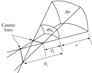
It can be useful to express d₀ and din terms of the curvature radii of the wavefronts. To this end, let us consider the general case of an astigmatic tube of rays shown in Fig. 2.3.

Figure 2.3 Astigmatic tube of rays.

The surfaces d₀ and d have principal radii of curvature ₁, ₂ and ₁s, ₂s, respectively, where s denotes the distance along

(18)

the ray path from P₀ to P. Since both d₀ and d subtend the same solid angle, it results:







0 1 2 1 2 d d s s          (2.6) or equivalently





1 2



0 1 2 E E s s        (2.7)

It is evident in Fig. 2.3 that rays focus (cross) at different points. As a matter of fact, the tube of rays degenerates into a line and the field intensity approaches infinity when s  or ₁ s  . The locus of ₂ points where this occurs is called caustic. It must be stressed that fields have always a finite value and, as a consequence, neither GO or GTD can be used to predict the field strength at caustic points.

As the phase variation along a ray is given by ks, the electric field along a ray can be written as follows:

0 ( ) jks

E E A s e (2.8)

wherein E₀ denotes the electric field at a reference point P₀ (s0),

k is the propagation constant and ( )A s is the spatial attenuation factor,

also known as spreading factor. This last reduces to the following expressions in the special case of plane wave (₁  ,₂  ), cylindrical wave (₁  ,₂ ) and spherical wave ( ₁ ,

2   ): 









1 plane- wave ( ) / cylindrical-wave / spherical-wave A s s s       _   _  (2.9)

(19)

2.2 Geometrical Optics 11 It is worth to note that when a caustic is crossed, _i changes s

the sign and this corresponds to a phase variation of π/2. Eq. (2.8) allows evaluating the field at a given point P in terms of its value at a reference point P₀. It has been derived by using the principle of conservation of energy in a tube of rays. Although it is a valid high frequency approximation for light waves, it could be not accurate for electromagnetic waves of lower frequencies.

2.2.2 Reflection from surfaces

GO laws such as Snell’s law can be used to determine the field reflected from surfaces. Let us consider a uniform plane wave impinging on a planar surface S assumed perfectly conducting. This case is illustrated in Fig. 2.4, where ˆsi and ˆsr denote the unit vectors in the incidence and reflection directions, respectively. The total field at the reflection point Q_r on S must meet the boundary condition:





ˆ i r 0

n E E  (2.10)

ˆn being the unit vector normal to S.

Figure 2.4 Reflection from a planar surface.

It is opportune to express the incident and reflected fields E and i E r

in terms of their components parallel and perpendicular to the incidence plane (that is the plane defined by ˆs and i ˆn):

(20)

ˆ ˆ i i i i i E E e_{ }E e_{ } (2.11) ˆ ˆ r r r r r E E e_{ } E e_{ } (2.12)

Equation (2.12) can be rewritten in a compact form:

r i r i E E R E_ E_                   (2.13) where 1 0 0 1 R_{ } _ 

  is the dyadic reflection coefficient for a perfectly conducting surface.

With reference to Fig. 2.4, ˆe_ is a unit vector normal to the incidence plane, and eˆ_i, eˆ_r are unit vectors parallel to the incidence plane defined by:

î î î

e_ e_s (2.14)

ˆr ˆ ˆr

e_ e_s (2.15)

In agreement with the principle of locality, the field reflected from a surface does not change when this last is no more planar, being always possible to consider the local plane tangent at Q_r. Obviously, the spreading factor changes to account for the variation of the reflected wavefront. Therefore, it is possible to express the reflected field as follows: ( ) ( ) ( ) r i jks r E s  R E Q A s e (2.16) wherein



1 1 2



2



( ) r r r _s r _s A s        (2.17)

(21)

2.2 Geometrical Optics 13 and s is the distance between the reflection point Q_r and the observation point P . In addition, ₁r and ₂r are the principal curvature radii of the reflected wavefront in Q_r. They are related to the principal curvature radii of the incident wavefront ₁i.  and to ₂i those relevant to the surface S (a and ₁ a ). It can be shown that ₂ ₁r

and ₂r are given by [2]:

1 1 2 1 1 1 1 1 1 2 r i i _f       _  _   (2.18) 2 2 1 2 1 1 1 1 1 2 r i i _f       _  _   (2.19)

wherein the parameters f and ₁ f in the particular but more ₂

interesting case of spherical wave incidence simplify to:

2 2 2 2 1,2 1 2 1 1 sin sin cos i f a a       _  _   2 2 2 2 1 2 1 2 1 sin sin 4 cos i a a a a       _  _   (2.20)

In eq. (2.20), i is the incidence angle, ₁ and  are the angles ₂ formed by ˆs and the directions associated to the principal radii of i

curvature of S. In the far field approximation, eq. (2.16) reduces to:

1 2 ( ) ( ) jks r i r r r e E s R E Q s      (2.21)

It is immediate to verify that in the case of plane wave incidence it results:

(22)

1 2r r a a1 2

   (2.22)

Accordingly, GO fails predicting the reflected field when one or both the curvature radii of S are infinite.

2.3 Diffracted Field

In agreement with eq. (2.8), the diffracted field can be expressed as:







( ) ( ') d d ' jks E s E O e s ' s        (2.23) ( ') d

E O being the diffracted field at a reference point O . It is ' convenient to choose the diffraction point Q as reference point. _d

Let us consider the case of diffraction from an edge which is, obviously, a caustic for the diffracted rays. Accordingly, the limit

0

lim d( )

' E O' '

  (2.24)

exists and is not zero. Moreover, the diffracted field must be proportional to the incident field in Q and thus it is possible to write: _d

0

lim d( ) i( _d)

' E O' ' DE Q

   (2.25)

wherein D is usually referred to as dyadic diffraction coefficient. As

a consequence, the field diffracted from the point Q on the edge is _d

given by: ( ) ( _d) d i jks E s DE Q e s      (2.26)

(23)

 being the distance between the caustic at the edge and the second caustic for the diffracted rays. In [2] it has been demonstrated that:

 

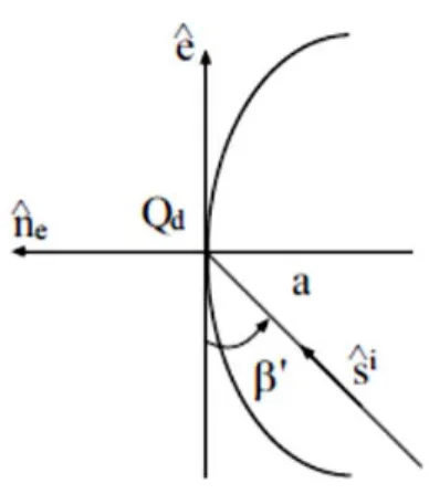
2 ˆ ˆ ˆ 1 1 sin i e i e n s s a '        (2.27)

where _ei is the curvature radius of the incident wavefront in Q_d, taken in the plane containing the incident ray and the unit vector ˆe tangent to the edge in Q_d (see Fig. 2.5). Moreover, a is the curvature radius of the edge and ˆn is the unit vector normal to the edge _e

directed away from the center of curvature. When the distance  is positive, the diffracted ray encounters no caustic along its path. Indeed, such a distance is negative only when the second caustic is located on the same side of the observation point. It is opportune to remark that the diffracted field expressed by eq. (2.26) is undefined at the caustic points and crossing such points implies a phase variation of π/2.

Figure 2.5 Diffraction from a curved edge.

In the case of vertex diffraction, diffracted rays are originated from a point caustic. Accordingly, it is possible to write:

0

lim d( ) i( _v)

' E O' ' DE Q

(24)

and the field diffracted from the vertex can be evaluated as: ( ) ( ) jks d i v e E s DE Q s   (2.29)

2.3.1 Diffraction by perfectly conducting surfaces

The canonical problem of plane wave diffraction by a perfectly conducting edge with planar surfaces has been treated by many authors but the most popular results have been presented by Keller [1]. The related diffraction coefficients are non-uniform, namely not valid at the GO shadow boundaries. This limitation has been overcome thanks to the solution provided by Kouyoumjian [2], [3].

Let us consider a radiating source at a point S in presence of a perfectly conducting wedge and observe the field at a point P. In accordance with the Fermat’s principle, the diffraction points can be determined by minimizing the distance SQ P . This leads to the law _d

of diffraction:

ˆ ˆ ˆ ˆi

s e s e   (2.30)

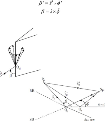
where ˆe is the unit vector directed along the edge, sˆi and ˆs are the unit vectors in the incidence and diffraction directions, respectively. As consequence of eq. (2.30), when a ray impinges on the edge at oblique incidence forming an angle  with respect to ' ˆe, the diffracted rays lie on a conical surface whose semi-aperture angle is still  . The incident ray direction is usually described by a couple of '

angles



  and the position of the diffracted ray on the cone is ', '



fixed by the angle  (Fig. 2.6).

As suggested by Kouyoumjian and Pathak, it is convenient to define the incidence plane (that containing the incident ray and the unit vector ˆe) and the diffraction plane (that containing the diffracted ray and the unit vector ˆe). A reference system in the incidence plane is introduced and fixed by the unit vectors ˆ' , ˆ ' , ˆs . In a similar i

(25)

2.3 Diffracted Field 17 diffracted ray. The unit vectors ˆ' and ˆ are perpendicular to the incidence and diffraction planes, respectively. The unit vectors ˆ ' and

ˆ

 are parallel to the incidence and diffraction planes and defined by: ˆ_' _s_ˆi ˆ_'

   (2.31)

ˆ ˆs

   (2.32)

Figure 2.6 Reflection and diffraction by a wedge.

When adopting these ray-fixed reference systems for describing the incident and diffracted fields, it results:

0 0 ( ) d d ' d d ' s jks h E D E e D s s E E          __ _   _{ } _      _ _      (2.33)

wherein D_{s h}_, are the scalar diffraction coefficients for the Dirichlet (soft) and Neumann (hard) boundary conditions, respectively.

(26)

The uniform diffraction coefficients for a perfectly conducting wedge [2] are reported in the following for reader’s convenience:

/4 , ( , ', ') 2 2 sin ' j s h e D n k          



'



_

_

cot ' 2n F kLa   _ _{ }       _ _ _ _ _{ }  _    



'



_

_

cot ' 2n F kLa          _{ } _  _ _{ }  _   



'



_

_

cot ' 2n F kLa          _{ } _   _{ } _    



'



_

_

cot ' 2n F kLa   _ _{ }       _ _ _   _{ } _     (2.34) where: 2 ( ) 2 jx j x F x j xe e  d   



(2.35)

is the UTD transition function, a and a are defined by:

2 2 2cos 2 n N x a  _   _   (2.36)

N being the nearest integers satisfying the following relation:

2n N   x (2.37)

The distance parameter L in (2.34) can be determined by imposing the continuity of the total field at the shadow boundaries [4], thus obtaining:

(27)











2 1 2 1 2 sin ' i i i e i i i e s s L s s            (2.38)

where ₁i, ₂i are the principal radii of curvature of the incident wavefront and _ei is the curvature radius of the incident wavefront taken in the incidence plane.

Diffraction coefficients for the half-plane can be easily found by setting n = 2 in eq. (2.34).

It can be easily verified that in correspondence of a shadow boundary one of the cotangent functions becomes singular whereas its product with the corresponding transition function is finite. Grazing incidence must be considered separately. In this case, D_s  and the 0 expression of D in eq. (2.34) must be multiplied by the factor 1/2. _h

When the wedge surfaces are curved (see Fig. 2.1), it is possible to consider in accordance with the principle of locality a wedge with planar surfaces tangent to the faces of the curved wedge. Moreover, the diffraction coefficients (2.34) can be still applied but the parameter

L must be properly modified to account for the curvature of the

reflected wavefront [2].

2.3.2 Slope diffraction

In addition to the edge diffraction contribution (2.33), it is often necessary to consider a higher order term which is proportional to the normal derivative of the incident field at Q . This contribution may _d

be not negligible when the amplitude of the incident field at Q is _d

small. Such type of diffraction is usually referred to as slope diffraction. By similar arguments, it is possible to consider high order slope diffraction terms. When only the first slope diffraction term is considered, the total diffracted field reads as:

 

1 ,

 

_{( )} ' s h i d jks d i d D U Q U U Q A s e jk  n        _ _ _{ } _      (2.39)

(28)

where U denotes a component of the diffracted field, _d D_{s h}_, /' are the slope diffraction coefficients and U_i/ is the normal derivative n

of the incident field in Q . Compact expressions for the slope _d

diffraction coefficients relevant to a perfectly conducting wedge can be found in [3].

2.3.3 Diffraction by finite conductivity surfaces: UTD

heuristic solutions

In the past years, the UTD has been successfully applied to solve a large variety of electromagnetic wave interaction problems with perfectly conducting surfaces, such as the analysis of radiation characteristics of simple and complex antenna systems [5]. However, its extension to finite conductivity structures is in general a non-trivial problem and still subject of continuing research. This interest is justified since in many application fields, such as radio propagation, Radar Cross Section (RCS) prediction, analysis of novel antenna systems, diffraction from not perfectly conducting objects is very frequent and the use of diffraction coefficients (2.34) could lead to inaccurate results. As a consequence, it is essential to have reliable solutions for the field diffracted by not perfectly conducting structures in order to make accurate field predictions. It is opportune to note that rigorous and exact diffraction coefficients have been developed for different surface impedance structures with the Maliuzhinets theory [6]. These are rather cumbersome and, due to their complexity, often not easy to use in routine applications such as propagation prediction tools. Thus, the difficulty arising in using such solutions forces simplifications to be made and to use approximate techniques.

Heuristic solutions have been proposed in the literature with reference to various scattering problems. They are not based on a rigorous solution of Maxwell’s equations but on a suitable modification to the diffraction coefficients (2.34) with the aim to compensate the geometrical optics field discontinuities at the shadow boundaries. Moreover, they are easy to handle and computationally simple. The problem of plane wave scattering by a thin lossless dielectric slab has been treated in both the normal and oblique incidence case [7]. The derived diffraction coefficients are an

(29)

2.4 Physical Optics 21 extension of diffraction coefficients for the perfectly conducting half-plane. Following the same idea in [7], two-dimensional diffraction coefficients have been proposed by Luebbers for the finite conductivity wedge [8] and are currently used in many ray tracing tools. Based on this solution, UTD slope diffraction coefficients have been later developed by the same author [9]. As discussed by Luebbers, the accurate use of these diffraction coefficients is restricted to applications involving wedges with large interior angles, and to the observation in proximity of shadow boundaries. Alternative heuristic UTD diffraction coefficients for not perfectly conducting wedges have been proposed in the recent years to improve the Luebbers’ solution accuracy within a wider angular region [10]-[12].

2.4 Physical Optics

The field scattered in the far zone by a perfectly conducting object illuminated by an electromagnetic wave is given by:









0 0 ˆ ˆ S ,

s

S

E  jk

_

I RR J G r r' dS (2.40) where J denotes the current distribution induced on the surface S of _s

the object, k₀ and ₀ are the wavenumber and the impedance of free space, _{G r r}_{( , ')}__ejk r r0  '



₄_ _{r r}_ _'



_{is the Green function and}_r_,

'

r denote the position vectors at the observation and integration points respectively, Rˆ is the unit vector from the radiating element at

'

r to the observation point and I is the (3×3) identity matrix.

Physical Optics approximates the current distribution J by using _s

geometrical optics and provides accurate results only when the object is far enough from the sources so that the incident field can be described in terms of wavefronts and rays. According to this approximation, the surface current is null in the shadow region. Whereas, at any point P on the object surface in the illuminated region it can be determined by assuming that the incident electric field is

(30)

reflected in the same way as it would be from the infinite plane tangent to the surface at P [13].

When the surface S is perfectly conducting, the surface current distribution can be evaluated according to:





ˆ ˆ 2ˆ

S i r i

J n H  n H H  n H (2.41)

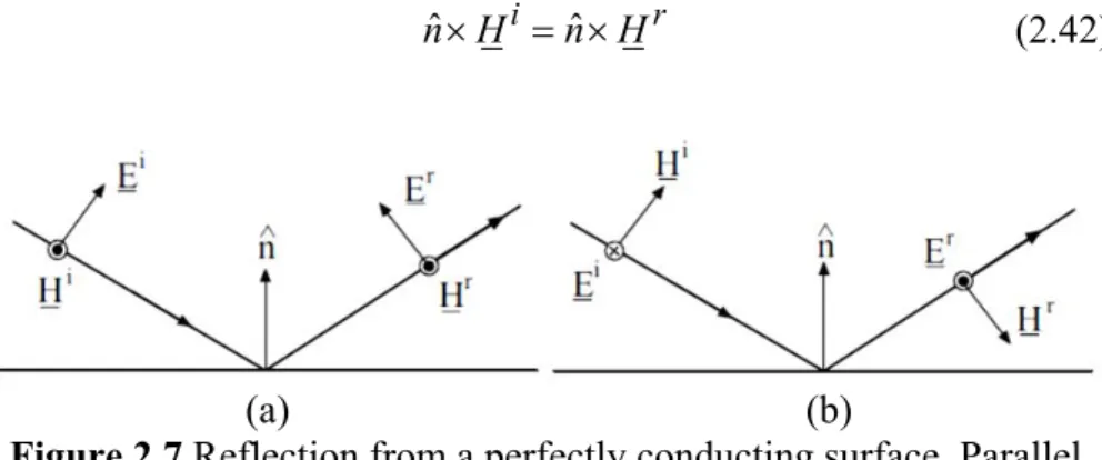
where ˆn is the unit vector normal to the surface at the incidence point and Hi is the incident magnetic field. As a matter of fact, when a plane wave impinges on a perfectly conducting surface, it results for both polarizations (see Figs. 2.7(a) and 2.7(b)):

ˆ i ˆ r

n H  n H (2.42)

(a) (b)

Figure 2.7 Reflection from a perfectly conducting surface. Parallel polarization (a). Perpendicular polarization (b).

PO can be also employed to evaluate the field scattered from finite conductivity objects. In such a case, both electric J_s and magnetic

ms

J surface currents must be taken into account in the radiation integral and so eq. (2.40) becomes:













0 ˆ ˆ 0 ˆ , s s ms S E  jk



_ I RR  J  J R G r r' dS_ (2.43) The accuracy of the results attainable with the PO method depends on the degree of approximation for the surface currents and on the observation direction. As a matter of fact, when the contributions due

(31)

2.5 Uniform Asymptotic Physical Optics approach 23 to the parts of the object not directly illuminated by the incident field are not negligible, some limitations in the field prediction are expected.

2.5 Uniform Asymptotic Physical Optics

approach

In the recent years, Uniform Asymptotic Physical Optics solutions have been developed to solve various diffraction problems [14]-[18]. The basic idea to obtain such solutions is the use of a PO approximation of the equivalent surface currents induced by an incident field on a structure. As well-known, the scattered field is expressed by means of the radiation integral (eqns. (2.40) and (2.43)) and it includes both the geometrical optics and the diffraction contributions. The application of the steepest descent method and a uniform asymptotic evaluation of the radiation integral allow deriving the diffraction coefficients in closed form. These last are expressed in terms of the UTD transition function and perfectly compensate the GO field discontinuities. It is opportune to point out that these solutions are inevitably approximate since the surface currents in the radiation integral are not exact but based on a PO approximation. In spite of this they are quite accurate when compared with more rigorous solutions and are simple, easy to handle and to implement. For these reason, they are potentially useful for practical applications when no exact analytical solutions are available or when these last cannot be evaluated in an efficient way. Although heuristic and efficient solutions have been proposed in the literature (see Subsec. 2.3.3) to solve diffraction problems having no exact solutions, they are not based on a rigorous analytical procedure and, therefore, should be used with considerable attention.

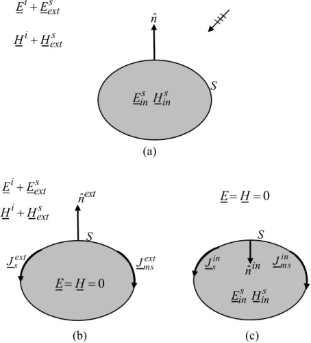
The key points showing how to construct a UAPO solution are reviewed in the following with reference to the problem of plane wave diffraction by a penetrable half-plane surrounded by free-space [18]. Let us consider the oblique incidence of an arbitrarily polarized plane wave over a penetrable half-plane surrounded by free-space (see Fig. 2.8). The incidence direction is fixed by the angles ' and  . In '

(32)

respect to the edge ( '  / 2 corresponds to the normal incidence). The observation direction is specified by the angles  and  . It is convenient to introduce the ray-fixed coordinate systems



sˆ, ' ˆ ˆ',



and



sˆ,  ˆ,ˆ



for the source and the observation points, respectively (see Fig. 2.8) and to assume the observation point P on the Keller’s diffraction cone, i.e.   '.

Figure 2.8 Diffraction by the half-plane edge.

At any observation point P, the total electric field E is given by the superposition of the incident field E and the scattered field i E . By s

applying the equivalence theorem, the surface currents induced by an incident plane wave on the surface S of the half-plane can be interpreted as sources of E and therefore, in the far-field s

approximation, the scattered field can be expressed by means of the following radiation integral

0 ( ˆ ˆ) 0 ˆ ( , ') s PO PO s ms S E  jk



_ I RR  J J R G r r dS_ (2.44) s^ b^ f^ x b' y z f' ^ b' s ' ^ ^ x

(33)

2.5 Uniform Asymptotic Physical Optics approach 25 in which the observation and source points are denoted by

ˆ ˆ ˆ ˆ

rx x y y z z    z z and r'x x z z'ˆ 'ˆ ' z z'ˆ.

By using a PO approximation for the equivalent electric and magnetic surface currents on S and expressing the fields in terms of their parallel and perpendicular components, it results:

0( 'sin 'cos ' 'cos ')

*

0JPOs 0J es jk x   z 

   (2.45)

0( 'sin 'cos ' 'cos ')

* jk x z PO

ms ms

J J e     (2.46)

and the three-dimensional Green function can be written as:

 





2 2 0 0 ' ' ' 2 2 ( , ') 4 ' ₄ _' _' jk z z jk r r e e G r r r r _{z z}               _ _ _{ } (2.47)

To evaluate the edge diffraction confined to the Keller cone for which

'

  , it is possible to approximate ˆR by the unit vector ˆs in the diffraction direction [19]

ˆ _ˆ _{sin 'cos} _ˆ _{sin 'sin} _ˆ _{cos '}_ˆ

R s    x   y  z (2.48) Accordingly, it results: * * 0 0 ˆˆ ˆ ( ) 4 s s ms jk E   _ I ss  J J  s_     





2 2 0 0 ' ' ' sin 'cos ' ' cos '

2 2 0 ' ' ' ' jk z z jk x z e e dz dx z z                    

 

* * 0 ˆˆ ˆ (I ss) Js Jms s Is   _    _ (2.49)

The expressions of the PO surface currents in terms of the incident electric field are here obtained by assuming such currents as

(34)

equivalent sources originated by the discontinuities of the tangential GO field components across the layer, i.e.,









ˆ ˆ PO i r t s S S J  y HH  y H H H 





0 ' sin 'cos ' ' cos ' 0 0 0 ˆ i r t jk x z y H H H e        (2.50)





ˆ





ˆ PO i r t ms S S J  EE  y E E E  y





0 ' sin 'cos ' ' cos ' 0 0 0 ˆ jk x z i r t E E E y e      _    _   (2.51)

As well-known, it is convenient to work in the standard plane of incidence and to consider the GO field components parallel () and perpendicular () to it. Therefore, it results:









0Js Ei Er Et cos ieˆ E Ei r E tt ˆ   _ _ _  _ _ _ _ (2.52)



i r t



cos iˆ



i r t



ˆ ms J  E E_ _ E_  e_ E_E_E t_ (2.53)

wherein E_i and E_i are the incident electric field components (at the origin) parallel and perpendicular to the ordinary plane of incidence,

i

 is the incidence angle in such a plane, eˆ_



s y s yˆ ˆ'



ˆ ˆ' is the unit vector normal to the ordinary plane of incidence, sˆ' being the unit vector of the incidence direction, and ˆt  y eˆ ˆ_. The reflected and transmitted field components can be expressed in terms of the incident field components by means of the reflection matrix R and transmission matrix T, and their expressions can be found in [18]. As well-known, in the high-frequency approximation, the PO integral (2.44) extended to S can be reduced asymptotically to a sum ₀

(35)

2.5 Uniform Asymptotic Physical Optics approach 27 points on S and an edge diffracted field contribution. To this end, it ₀

is necessary to perform the evaluation of the following integral:

0 4 s jk I      





2 2 0 0 0 ' ' ' sin 'cos ' ' cos '

2 ₂ 0 e ' ' ' ' jk z z jk x _e jk z e _{dz dx} z z                   



(2.54)

As reported in [19], by making the substitution z z'    ' sinh

and using one of the integral representations of the zeroth order Hankel function of the second kind H₀(2) it results:

 





2 2 0 0 ' ' ' cos ' 2 2 ' ' ' jk z z jk z e e dz z z                







0 cos ' (2) 0 0 ' sin ' jk z j e  H k        (2.55)

The involved Hankel function can be now written with the useful integral representation





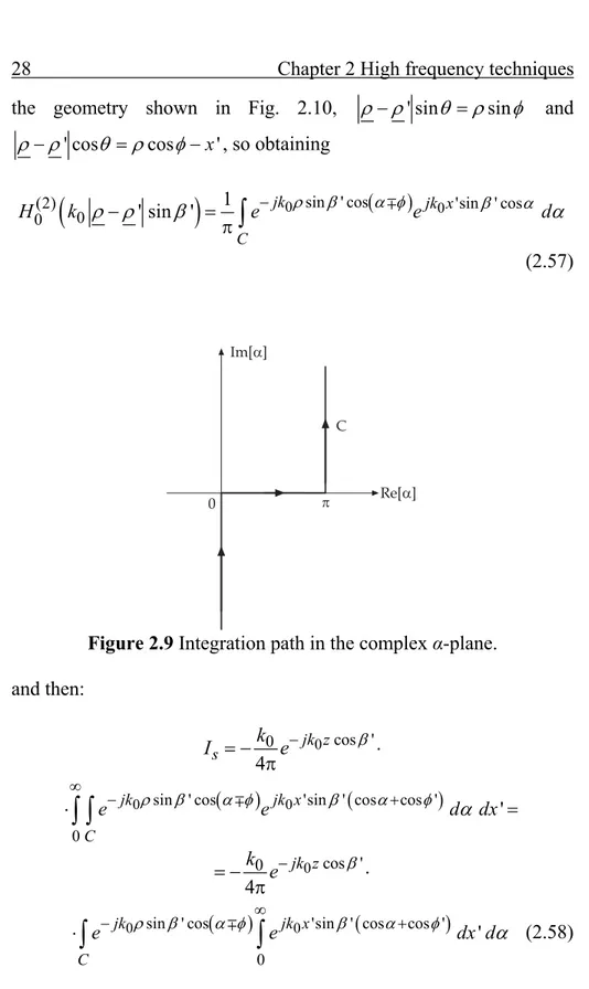
0 ' sin ' cos  (2) 0 0 1 ' sin ' jk C H k     e      d 



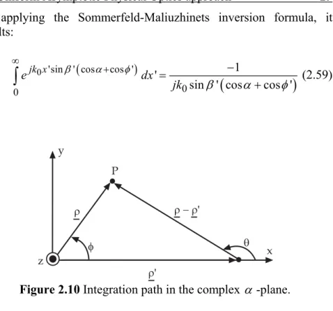
 (2.56)

where C is the integration path in the complex  -plane (see Fig. 2.9). The angle  is between the illuminated face and the vector   , ' and the sign  (+) applies if y (0 y ). If 0    , according to

(36)

the geometry shown in Fig. 2.10,   ' sin  sin and ' cos cos x'      , so obtaining





0 sin ' cos  0 (2) 'sin ' cos 0 0 1 ' sin ' jk jk x C H k     e     e   d 



 (2.57)

Figure 2.9 Integration path in the complex α-plane. and then: 0 cos ' 0 4 jk z s k I   e       

0 sin ' cos 0 'sin ' cos cos '

0 ' jk jk x C e     e    d dx    

_{ }

  0 cos ' 0 4 jk z k e         

0 sin ' cos 0 'sin ' cos cos '

0 ' jk jk x C e     e    dx d    

_



_

(2.58) Re[a] Im[a] C 0 p

(37)

2.5 Uniform Asymptotic Physical Optics approach 29 By applying the Sommerfeld-Maliuzhinets inversion formula, it results:

 





0 'sin ' cos cos '

0 0

1 '

sin ' cos cos '

jk x e dx jk         _  



(2.59)

Figure 2.10 Integration path in the complex  -plane. so that

 

0

0 cos ' ₁ sin ' cos

2sin ' 2 cos cos '

jk jk z s C e e I d j             



  (2.60)

where the sign  (+) applies in the range 0   (     ). Such  2 an integral can be evaluated by using the Steepest Descent Method [19]. To this end, the integration path C is closed with the Steepest Descent Path (SDP) passing through the pertinent saddle point  as _s shown in Fig. 2.11. According to the Cauchy residue theorem, the contribution related to the integration along C (distorted for the presence of singularities in the integrand) is equivalent to the sum of the integral along the SDP and the residue contributions Res_i

 

_p

associated with all those poles that are inside the closed path C+SDP, i.e., r - r' r y P f q r' x z

(38)

 

1

 

  2 f s C I g e d j        



 

  SDP 1 Re 2 f i p i s g e d j         





 

Re _i _p i s  I 



  (2.61) in which

 

  SDP 1 2 f I g e d j         



 

    SDP 2 s s f f f e g e d j  _ _    _ _ _  _   



(2.62)

 

e 0 cos ' 1

2sin ' cos cos ' cos cos '

jk z _A g             (2.63) 0 k 

  and f

 

  jsin ' cos



 



. Note that  is typically large, _p   and ' _s  (_s   2 ) if 0   (     2 ). Moreover, by putting   ' j" and imposing that

 

Im_f  _Im_f _s _ and Re_f

 

 _Re_f

 

_s _, the considered SDP is described by:





1 1 ' sgn( '')cos ( '') cosh '' s s gd            (2.64)

where gd

 

" is the Gudermann function. By using now the change of variable f

 

  f

 

_s  20, eq. (2.62) can be written as

(39)

2.5 Uniform Asymptotic Physical Optics approach 31

 

2 I G  e  d      

_

(2.65) wherein

 

₂1



 



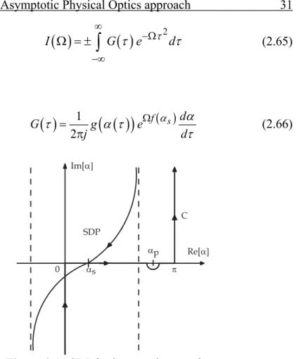
f s d G g e j d          (2.66)

Figure 2.11 SDP in the complex  -plane.

When _p is approaching  , the function _s G

 

 cannot be expanded in a Taylor series. To overcome this drawback it is convenient to regularise the integrand in (2.65) using the Multiplicative Method. It requires introducing the regularised function

 





 

p p G     G  (2.67) with

 





2 _{sin ' 1 cos} _' p f s f p j         _    _ Im[a] Re[a] C SDP 0 _as ap p

(40)

2 ' 2 sin 'cos 2 j     j   _ _    (2.68)

and  is a measure of the distance between _p and  . Accordingly, _s

 

p

 

2 p e I G   d         



(2.69)

Since G_p

 

 is analytic near  0, it can be expanded in a Taylor series. By retaining only the first term (i.e., the 1 2-order term) since  1, it results:

 

_{ }

p

 

0



2



t p p G I  F j                 (2.70) in which

 

  0 0 ₁ 0 2 s p f s p G _d G g e j d              sin ' 4 1 2

2 cos cos ' sin '

j j A e e j           _ _   _ _ (2.71) and

 

2 j j 2 t F j e  e  d     



  (2.72)

is the UTD transition function [2]. By substituting (2.68) and (2.71) in (2.70), the explicit form of the asymptotic evaluation of I

 

 is:

(41)

2.5 Uniform Asymptotic Physical Optics approach 33

 

4 0



_

sin ' cos '

_



0 sin ' cos cos '

2 2 sin ' jk z j e e I k                  2 0 ' 2 sin 'cos 2 t F  k       _ _ __    





0 4 2 0 1

2 2 sin ' cos cos '

jk s j e e k s           2 2 0 ' 2 sin 'cos 2 t F  k s      _ _ __     (2.73)

where the identities ssin ' and z s cos ' are used on the diffraction cone. The above analytic result contributes to the UAPO diffracted field to be added to the GO field and is referred to as a uniform asymptotic solution because I

 

 is well-behaved when

p s

  . In the GTD framework, the matrix formulation for the scattered field can be written as

' ' s i s s s i E E E M I E E                       (2.74)

As a consequence the UAPO edge diffraction contribution Ed is:

 

0 ' ' ' ' d i i _{jk s} d d i i E E E _e E M I D s E E E                                    (2.75)

where the UAPO solution for the 2 2 diffraction matrix

' ' ' ' D D D D D          _ _    

(42)

11 12

21 22 0

/4 2

1

2 2 sin (cos cos )

j M M e M M k '  '       _ _        2 2 0 2 sin cos 2 t ' F  k s '     _ _ __     (2.76)

where the sign () applies if 0   (     ). The explicit  2 expression of the coefficients M (i, j = 1, 2) can be found in [18]. _ij

Accordingly, the UAPO solutions have the same ease of handling of those derived in the UTD framework and, in addition, they have the inherent advantage of providing the diffracted field from the knowledge of the GO response of the structure. In other words, it is sufficient to make explicit the reflection and transmission coefficients related to the considered structure for obtaining the UAPO diffraction coefficients.

(43)

(44)

Chapter 3 High frequency diffraction by an

arbitrary-angled dielectric wedge

The problem of diffraction by a dielectric wedge has great relevance for practical applications. The accurate path loss prediction in radio wave propagation environments requires a correct characterization of diffraction contributions arising from the presence of edges and corners. However, the research activity focused mainly on impenetrable structures at high frequency and rigorous solutions have been reported in the literature for perfectly conducting wedges or impedance wedges. Starting from these solutions, there have been some attempts to extend their validity to the penetrable structures. This methods result to be complicated and manageable just for simple configurations, so it has been necessary to build up new approaches for this kind of problems. The lack of an exact and, at the same time, computationally efficient solution which can be employed in ray tracing tools forces simplifications to be made and to apply approximate solutions.

The aim of this chapter is to provide a UAPO solution for the field diffracted by the edge of a lossless arbitrary-angled dielectric wedge in the case of normal incidence. The solution is derived by means of the decomposition of the considered scattering problem into two sub-problems relevant to external and internal regions of the wedge. For each of them, proper equivalent currents, which can be interpreted as sources for the scattered fields, are determined by taking into account the penetrable nature of the structure. Then, uniform asymptotic evaluations of the radiation integrals allow deriving closed form expressions for the diffracted field. As demonstrated by numerical examples, the here developed UAPO solution compensates the GO field discontinuities in the exterior and interior regions. Furthermore,

(45)

3.1 Diffraction by dielectric wedges: state of the art 37 its accuracy is confirmed by the good agreement attained with results provided by numerical methods.

3.1 Diffraction by dielectric wedges: state of the

art

The problem of plane wave diffraction by wedges has received great attention due to the importance of its solutions in radio propagation planning, analysis and design of radiating structures and waveguide theory. The first studies have concerned wedges with perfectly conducting surfaces [2], [6] or impedances faces [14], [20], [21]. Heuristic solutions have also been proposed in [8], [9] for solving diffraction problems in the case of dielectric structures. Although efficient, they are not based on a rigorous analytical procedure and, therefore, should be used with considerable attention.

Rawlins [22] presented an approximate solution for the field produced when an electromagnetic plane wave is diffracted by an arbitrary-angled dielectric wedge, whose refractive index is near unity. It was obtained from an application of the Kontorovich-Lebedev transform and a formal Neumann-type expansion. The results were in agreement with those derived by the same author with reference to a right-angled wedge [23]. The diffracted field of an E-polarized plane wave by a dielectric wedge was formulated in terms of integral equations by Bernsten in [24]. These were transformed into Fredholm integral equations and solved by iterative methods for limited values of the dielectric constant. Joo et al. [25] proposed an asymptotic solution for the field diffracted by a right-angled dielectric wedge based on a correction of PO approximation to the edge diffraction. The correction in the far-field zone was calculated by solving a dual series equation agreeable to simple numerical evaluation. The extension of the approach to arbitrary-angled wedges was addressed in two companion papers [26] and [27]. Burge et al. [28], starting from a PO version of the GTD, provided an edge coefficient for the external and internal diffraction by an arbitrary-angled dielectric wedges. Rouviere et al. in [29] improved the Luebbers’ heuristic solution

[8] in the UTD framework [2] by adding two new terms that compensate the discontinuity created by the field transmitted through the structure. Another heuristic solution for the diffraction coefficient

(46)

of a penetrable wedge has been proposed in [30] by Bernardi et al.. It is obtained by a modification of the exact UTD diffraction coefficient related to the metallic wedge.

The FDTD method was applied in [31] and [32], providing numerical results for the diffraction coefficient of right-angled wedges made of perfect electrical conductor (PEC), lossless dielectric and lossy dielectric material.

Another interesting attempt to solve the problem of the diffraction by a right-angled dielectric wedge was proposed by Radlow [33]. He used multidimensional Wiener-Hopf equations to model the problem, but the factorization of these equations needs function-theoretic techniques employing two complex variables that are cumbersome to handle. Bates [34] introduced iterative formulas to obtain a set of basic wave-functions useful to represent the sources situated on the plane of symmetry of an arbitrary-angled dielectric wedge. Seo and Ra [35] proposed a remarkable methodology to evaluate the scattering from a lossy dielectric wedge: reflected and refracted GO fields are obtained by inhomogeneous plane wave tracing in the lossy medium, while PO approximation in the edge diffracted fields are accurately corrected by adding the multipole line sources at the edge of the wedge to satisfy the extinction theorem. The unknown expansion coefficients used at the tip of the wedge to make disappearing the extinction integral are evaluated numerically. Salem et al. [36] extended Rawlins’ approach [22] to a more general form of excitation (line source) of a dielectric wedge. They expressed the Kontorovich-Lebedev transform functions as a Neumann series and represented the scattered field as a Bessel function series, so extending solutions to the case of real valued wavenumbers and arbitrarily positioned source and observer. Daniele and Lombardi [37] analyzed the problem of diffraction of an incident plane wave by an isotropic penetrable wedge in the general case of skew incidence. They used generalized Wiener-Hopf equations, and the solution is obtained using analytical and numerical-analytical approaches that reduce the Wiener-Hopf factorization to Fredholm integral equations of second kind. Vasilev et

al. [38], [39] developed a numerical approach based on the method of

integral equations to solve the problem. They represented the unknown surface currents on the dielectric wedge as a sum of uniform and non-uniform components (using the Ufimtsev’s method), making

(47)

3.2 Diffraction by an arbitrary-angled dielectric wedge 39 possible the derivation of the numerical solution. Budaev [40] developed a hybrid methodology to solve the problem of diffraction by a dielectric wedge in an exact sense, which combines analytical and numerical techniques.

UAPO solutions were proposed in explicit closed form in [41] and [42] for evaluating the field diffracted by right- and obtuse-angled lossless dielectric wedges in the inner and outer regions. The UAPO-based approach has been also applied to acute-angled wedges in [43] considering a specific range of incidence directions for both cases of

E- and H-polarized plane wave. Then, in [44] the analysis has been

extended to all possible cases of incidence direction providing generalized UAPO solutions which are valid for the diffraction by a wedge with arbitrary aperture.

3.2 Diffraction by an arbitrary-angled dielectric

wedge

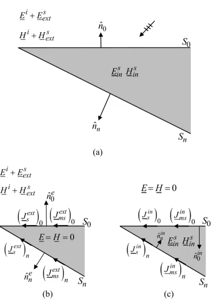
In this section the UAPO solutions for the diffracted field originated by an arbitrary-angled lossless dielectric wedge are determined for an incident plane wave. The geometry used as reference in the following is relevant to a wedge having an acute internal apex angle. This choice is justified by the complexity of the propagation mechanisms (multiple internal and external rays) which include those concerning right- and obtuse-angled wedges [41], [42], as will be demonstrated at the end of this chapter.

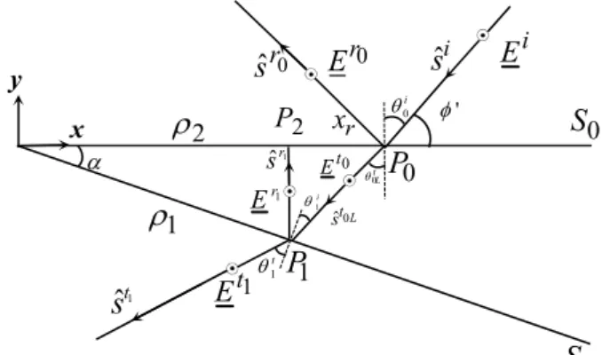
Let us consider the problem of the diffraction of an E-polarized plane-wave by the edge of an acute-angled dielectric wedge (see Fig. 3.1). Its internal apex angle is  and its material is lossless, non-magnetic (_r 1), with relative permittivity  and propagation _r constant k_d k_d _r . The wedge surfaces are denoted by S₀ and S_n. A Cartesian reference system



x y z is introduced with the y-axis , ,



normal to the face S₀ and the z-axis directed along the edge. The incidence direction is assumed perpendicular to the edge (see Fig. 3.1) and defined by the angle ' ( ' 0  corresponds to the grazing incidence with respect toS₀).

(48)

Figure 3.1 Geometry of the diffraction problem.

The observation point is denoted by ( , )P   . The structure divides the space in two regions: the exterior region



0    2 



and the interior region



2     .   2



3.2.1 GO field model for 0 < ϕ′ < π/2

Closed form expressions for the GO response when 0     are '

derived in this section.

Only the face S₀ is directly illuminated by the incident field. A transmitted ray exists in the inner region and, in absence of total internal reflection on S_n, it is transmitted through this last. The reflected ray travels toward S₀ and gives rise to following reflection and transmission mechanisms involving S₀ andS_n. When the value of the internal angle of incidence makes to occur the inversion the rays begin to go far from the apex. Accordingly, two series of internal and external rays exist: the first contains rays (black arrows in Fig. 3.2) travelling towards the apex and the second comprises those (red arrows in Fig. 3.2) going far from the apex, as illustrated in Fig. 3.2. The external rays exist until the internal total reflection doesn’t occur. The number of pre- and post-inversion rays is determined by the values of ' ,  and  . In order to better understand the ray _r propagation inside and outside the wedge, the reader can refer to Fig. 3.3. If ₀i    is the external incidence angle, the wave 2 '

Diffraction by dielectric wedges: high frequency and time domain solutions

Facoltà di Ingegneria

T

D