Self Tuning Control Techniques for a Wind Turbine System and a Hydroelectric Plant

ISSN Online: 2327-5901 ISSN Print: 2327-588X

Self-Tuning Control Techniques for Wind

Turbine and Hydroelectric Plant Systems

Silvio Simani

*

, Stefano Alvisi, Mauro Venturini

Department of Engineering, Ferrara University, Ferrara, Italy

Abstract

The interest on the use of renewable energy resources is increasing, especially towards wind and hydro powers, which should be efficiently converted into electric energy via suitable technology tools. To this aim, self-tuning control techniques represent viable strategies that can be employed for this purpose, due to the features of these nonlinear dynamic processes working over a wide range of operating conditions, driven by stochastic inputs, excitations and disturbances. Some of the considered methods were already verified on wind turbine systems, and important advantages may thus derive from the appro-priate implementation of the same control schemes for hydroelectric plants. This represents the key point of the work, which provides some guidelines on the design and the application of these control strategies to these energy con-version systems. In fact, it seems that investigations related with both wind and hydraulic energies present a reduced number of common aspects, thus leading to little exchange and share of possible common points. This consid-eration is particularly valid with reference to the more established wind area when compared to hydroelectric systems. In this way, this work recalls the models of wind turbine and hydroelectric system, and investigates the appli-cation of different control solutions. Another important point of this investi-gation regards the analysis of the exploited benchmark models, their control objectives, and the development of the control solutions. The working condi-tions of these energy conversion systems will also be taken into account in order to highlight the reliability and robustness characteristics of the devel-oped control strategies, especially interesting for remote and relatively inac-cessible location of many installations.

Keywords

Wind Turbine System, Hydroelectric Plant Simulator, Model-Based Control, Data-Driven Approach, Self-Tuning Control, Robustness and Reliability How to cite this paper: Simani, S., Alvisi,

S. and Venturini, M. (2019) Self-Tuning Control Techniques for Wind Turbine and Hydroelectric Plant Systems. Journal of Power and Energy Engineering, 7, 27-61.

https://doi.org/10.4236/jpee.2019.71003

Received: December 12, 2018 Accepted: January 18, 2019 Published: January 21, 2019 Copyright © 2019 by author(s) and Scientific Research Publishing Inc. This work is licensed under the Creative Commons Attribution International License (CC BY 4.0).

http://creativecommons.org/licenses/by/4.0/

Open Access

1. Introduction

The trend to reduce the use of fossil fuels, motivated by the need to meet green-house gas emission limits, has driven much interest on renewable energy re-sources, in order also to cover global energy requirements. Wind turbine sys-tems, which now represent a mature technology, have had much more develop-ment with respect to other energy conversion systems, e.g. for biomass, solar, and hydropower [1]. In particular, hydroelectric plants present interesting ener-gy conversion potentials, with commonalities and contrast with respect to wind turbine installations [2] [3].

One common aspect regarding the design of the renewable energy conversion system concerns the optimality and the efficiency of its converter. However, as wind and hydraulic resources are free, the key point is represented by the mini-misation of the cost per kWh, also considering the lifetime of the deployments. Moreover, when the capital, operational and commissioning/decommissioning costs are fixed, the value of the energy sold (i.e. the energy receipts) has to be maximised. This represents a fundamental economic objective, which should be carefully taken into account also by the design of the control system.

It is worth noting that preliminary works highlighted interactions between the renewable energy conversion system design and the strategies exploited to con-trol them, see for example, [4]. Moreover, by taking into account that the cost of control system technology (i.e. sensors, actuators, computer, software) is rela-tively lower than the one of the renewable energy converter [5], the control sys-tem should aim at increasing the energy conversion capacity of the given plant. However, this strategy neglects the control system capability and the engineering expertise required for the development of a suitable control technique. As an example, model-based control design schemes need for a high-fidelity mathe-matical model of the process to be controlled, which could have required a sig-nificant number of man-hours to achieve it.

It is quite established that the mathematical descriptions of both wind turbine processes and hydroelectric plants are represented by nonlinear dynamic processes working over a wide range of operating conditions and excitations. These systems are also required to operate under specific physical constraints, such as displacements, velocities, accelerations, torques and forces. Therefore, these systems can operate effectively with economically attractive and high op-erational lifetimes only if their working conditions are carefully fulfilled. With these issues in mind, the paper recalls the mathematical description of a wind turbine system and a hydroelectric plant, by using a wind turbine benchmark and a hydroelectric simulator, respectively. The former process was proposed for the purpose of an international competition started in 2009 and described in de-tail [6], whilst the latter system was developed by the same authors, and pre-sented for the first time in [7]. On the other hand, this work analyses different control strategies for both wind turbines and hydroelectric systems that can show common and different aspects. Moreover, in general, when considering DOI: 10.4236/jpee.2019.71003 28 Journal of Power and Energy Engineering

on-grid plants, the control system has to consider also the regulation of the vol-tage and frequency, which will not be addressed in this work.

After these remarks, by means of the analysis of the proposed modelling and control topics, the work will sketch common and different aspects of wind tur-bines and hydraulic systems, which will be exploited for the design of the control technique. On one hand, hydroelectric power plants result to be more estab-lished and even more common than wind turbine processes, but the control as-pects for the latter systems have been examined more in depth in the last dec-ades.

With reference to wind turbine systems, it can be observed that modern in-stallations exploit control techniques and technologies in order to obtain the needed goals and performance achievements. These plants can implement their regulation via “passive” control methods, such as the plants with fixed-pitch, and stall control machines. The blades of these systems are deployed in order to limit their power via the blade stall, when the wind speed exceeds its rated value. These systems do not need any pitch control mechanism, as addressed e.g. in [8]. Moreover, these plants implement a simple rotational speed control, thus avoiding the inaccuracy problems derived from the measurement of the wind speed [9]. On the other hand, wind turbine rotors using adjustable pitch systems are often exploited in constant-speed installations, in order to overcome the li-mitations due to the simple blade stall and to improve the converted power [10]. Therefore, in order to increase the generated power below the rated wind speed, the wind turbine has to modify its rotational speed with the wind velocity. To this aim, the regulation of the blade pitch is exploited only above the rated wind speed to control the generated power [11].

It is worth noting that a limited number of works have addressed the devel-opment of self-tuning control techniques for hydroelectric plants, as shown e.g. in [12]. In fact, a high-fidelity mathematical description of these processes can be difficult to be achieved in practice. However, some contributions reported the analytical formulation of hydroelectric plants, together with the design of their control strategies. Note that these papers took into account the elastic water ef-fects, even if the nonlinear dynamics are linearised around an operating condi-tion. Moreover, other contributions, see e.g. [13], proposed different mathemat-ical models together with the strategies exploited to control these systems.

In the light of these considerations, the paper also proposes to analyse those control aspects that might be similar between wind turbine and hydroelectric systems, with the aim of exploiting some solutions, developed in the wind tur-bine domain, and to apply them within the other concerning hydroplants. This approach could be used to stimulate novel research topics and the development of innovative techniques in a multidisciplinary control community, and the most important achievements will be summarised in this paper. In particular, suitable analytical models of these energy conversion plants should be able to provide the overall dynamic behaviour of the monitored processes, thus leading impor-tant impacts on the development of the control techniques. Moreover, the work DOI: 10.4236/jpee.2019.71003 29 Journal of Power and Energy Engineering

introduces some kind of common rules for tuning the different controllers, for both wind turbine and hydroelectric plants. Therefore, the paper shows that the parameters of these controllers are obtained by exploiting the same tuning strat-egies. This represents one of the key contributions of the study.

Note that some previous studies by the same authors addressed several topics presented in this paper. For example, the work [7] considered control techniques when applied only to the hydroelectric simulator, which were not compared to the wind turbine benchmark. On the other hand, the paper [14] performed an overview of the main modelling and control strategies, in particular for wind turbines and wave energy devices: the hydroelectric plant benchmark and the simulations of the proposed control techniques were not addressed. Moreover, the earlier work [7] presented the hydroelectric simulator, but considered only the design of standard PID regulator for the optimisation of its time response.

It is worth highlighting the main contribution of the paper, which aims at providing some guidelines on the design and the application of self-tuning con-trol strategies to two energy conversion systems. Some of these techniques were already verified on wind turbine systems, and important advantages may thus derive from the appropriate implementation of the same control methods for hydroelectric plants. In fact, it seems that investigations related with both wind and hydraulic energies present a reduced number of common aspects, thus leading to little exchange and share of possible common points. This considera-tion is particularly valid with reference to the more established wind area when compared to hydroelectric systems. In this way, the paper summarises also the most common models used for describing wind turbine and hydroelectric sys-tems. Moreover, it analyses the application of the different control solutions to these energy conversion systems. The aim is thus to exploit common points in the control objectives and the achievable results from the application of different solutions. The working conditions of these energy conversion systems will be also taken into account in order to highlight the reliability and robustness cha-racteristics of the developed control strategies.

Finally, the paper has the following structure. Section 2 provides the brief presentation of the benchmark and simulation models used for describing the accurate behaviour of the dynamic processes. Section 3 discusses the specific re-quirements of the control systems exploited to control these energy conversion plants. Section 3 summarises the design of the proposed model-based and da-ta-driven control techniques, taking into account the control objectives and the available tools. In Section 4, these self-tuning control strategies are implemented and compared, with respect to the achievable reliability and robustness features. Section 5 ends the paper summarising the main achievements of the paper, and drawing some concluding remarks.

2. Simulator Models and Reference Governors

This section recalls the simulators used for describing the dynamic behaviour of DOI: 10.4236/jpee.2019.71003 30 Journal of Power and Energy Engineering

the wind turbine and the hydroelectric processes considered in this paper. Moreover, the baseline control schemes developed for the regulation of the wind turbine benchmark are also summarised in Section 2.1. On the other hand, the hydroelectric simulator, together with its reference governor, is recalled in Sec-tion 2.2.

2.1. Wind Turbine System Benchmark

Industrial wind turbine installations are normally equipped with large rotors, flexible blades and light load-carrying structures, which work in uncertain envi-ronments, often placed in remote and inaccessible places [9]. These topics have motivated the use of high-fidelity simulators and the development of proper control solutions, which could cope with these challenging technologies. These control strategies should thus be able to obtain prescribed performances with respect to given set-points. Therefore, this paper will consider the design and the application of self-tuning control techniques that are able to optimise the track-ing of a given reference. This reference or set-point signal guarantees the max-imisation of the energy production [4].

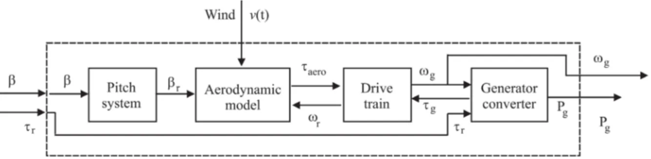
In particular regarding wind turbines, this work focuses on a horizontal-axis device, which nowadays represents the most common type of installation for large-scale deployments. Moreover, the three-bladed horizontal axis wind tur-bine model reported in this work follows the principle that the wind power acti-vates the wind turbine blades, thus producing the rotation of the low speed rotor shaft. In order to increase its rotational speed generally required by the generator, a gear-box with a drive-train is included in the system. A more detailed descrip-tion of this benchmark that was proposed for different purposes is provided in [9]. The schematic diagram of this benchmark that helps to recall its main va-riables and function blocks developed in the Simulink environment is depicted in Figure 1, also showing its working principles.

The wind turbine simulator presents 2 controlled outputs, i.e. the generator rotational speed ωg

( )

t and its generated power P tg

( )

. The wind turbine model is controlled by means of two actuated inputs, i.e. the generator torque

( )

g t

τ and the blade pitch angle β

( )

t . The latter signal controls the blade ac-tuators, which can be implemented by hydraulic or electric drives. The bench-mark considered in this work includes a hydraulic circuit actuating the

Figure 1. Block diagram of the wind turbine plant.

wind turbine blades [9].

Several other measurements are acquired from the wind turbine benchmark: the signal ωr

( )

t represents the rotor speed and τr

( )

t is the reference torque. Moreover, aerodynamic torque signal τaero

( )

t is computed from the wind speed v t

( )

, which is usually available with limited accuracy. In fact, the wind field is not uniform around the wind turbine rotor plane, especially for large ro-tor systems. Moreover, anemometers measuring this variable are mounted be-hind the rotor on the nacelle. Therefore, the wind speed measurement v t

( )

is affected by the interference between the blades and the nacelle, as well as the turbulence around the rotor plane. Furthermore, when these instantaneous wind fields are considered across the rotor plane, the wind variable v t

( )

may change in space and time, and it is especially true in large rotor installations. The altera-tion of the wind speed measurement v t

( )

with respect to its nominal value around the rotor plane represents an uncertainty in the wind turbine model and a disturbance term in control design. On the other hand, the aerodynamic tor-que depends on another factor, Cp, representing the power coefficient, as shown by Equation (1):

( )

(

( ) ( )

,

_{( )}

)

3

( )

2 p aero r AC t t v t t t ρ β λ τ ω =

(1)

ρ being air density, A the area swept by the turbine blades during their rota-tion, whilst λ

( )

t represents an important variable, i.e. the tip-speed ratio of the blade, which is given by the relation of Equation (2):

( )

_t r

( )

_{( )}

t R

v t

ω λ =

(2) where R is the rotor radius. The nonlinear static function C ⋅p

( )

represents the power coefficient, which is usually modelled via a two-dimensional map (or look-up table) [9]. The relation of Equation (1) is exploited to derive the variable

( )

aero t

τ _{assuming an uniform measurement} v t

_{( )}

, together with the acquired signals β

( )

t and ωr

( )

t . As remarked above, the uncertainty affecting the wind speed v t

( )

leads to an error in the derivation of the variable τaero

( )

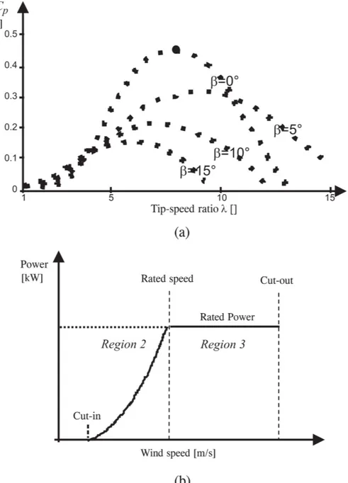
t [9]. Moreover, the overall nonlinear behaviour represented by the relations of Equa-tions (1) and (2) is reported in Figure 2. The picture is sketched for different values of the variable λ

( )

t _{, depending on the signals} v t

( )

and β

( )

t .

It is worth noting that diagram in Figure 2(b) represents the power curve highlighting the working conditions of the wind turbine system, also known as partial load (region 2) and full load (region 3) operating situations of the plant [9].

The wind turbine benchmark considered in this work includes a simple two-body linear model of the third order that is exploited to describe the dy-namic behaviour of the drive-train. It implements also a simple first-order linear dynamic model of the electric generator and a second order dynamic description of the pitching system, as addressed in more detail in [9]. The overall DOI: 10.4236/jpee.2019.71003 32 Journal of Power and Energy Engineering

Figure 2. Examples of power coefficient function (a) and power curve (b).

continuous-time representation of the wind turbine benchmark is represented by the general model in form of Equation (3):

( )

(

( ) ( )

)

( )

( )

, c x t f x t u t y t x t  =   =  

(3) with u t

( )

= τr

( ) ( )

t β t  and T

( )

( )

( )

T g g

y t _{= }ω t P t _{ are the manipulated}

input signals and the controlled output measurements, respectively. f ⋅c

( )

is described by means of a continuous-time nonlinear function that will be ex-ploited for representing the complete dynamic behaviour of the controlled process. Moreover, since this paper will analyse several data-driven control approaches, this system will be used to acquire a number of N sampled data sequences u k

( )

DOI: 10.4236/jpee.2019.71003 33 Journal of Power and Energy Engineering

and y k

( )

, with

k

=

1,2, ,

_

N

_{. Furthermore, the variables and parameters of} the wind turbine benchmark submodels (see e.g. Figure 1), the static function

(

,

)

p

C β λ , as well as the errors and uncertain effects affecting the input-output measurements were implemented in the simulation code in order to provide a high-fidelity wind turbine plant simulator, as highlighted in [9]. In particular, the input and output measurements, which are acquired from the wind turbine benchmark, are assumed to be actuated and measured by realistic devices intro-ducing additive Gaussian noise processes with zero mean and standard deviation values summarised in Table 1 [9].

As already highlighted by Figure 2(b), the wind turbine control task depends on its working conditions [9]. However, as the wind turbine benchmark recalled in this work operates in nominal conditions, only 2 regions are analysed, as re-marked above. In particular, when operating in the working region 2, the tur-bine is regulated to achieve the optimal power production (below the rated wind speed). On one hand, with reference again to Figure 2(b), this is obtained with the blade pitch angle

β

fixed to 0 degrees. On the other hand, the tip-speed ra-tio λ _{of Equation (2) is settled at its optimal value} K_opt. These conditions are obtained according to the peak value of the power coefficient function of the wind turbine, already represented in Figure 2(a). In this optimal working condi-tion, the reference torque equals the converter one, i.e. τg =τr, as described by the relation of Equation (4):

2

r Kopt r

τ

=

ω

(4) In this situation, the optimal tracking of the power reference is obtained, as soon as the wind speed v t

( )

increases, and the working condition moves to the control region 3. The control task aims also at tracking the power reference Pr, which is achieved by modifying

β

, while Cp is decreasing. The advanced control strategies considered in this work tries to maintain the generator speed

g

ω at its nominal value ωnom by changing both

β

and τg.

Therefore, the control system operating in region 2 exploits the relations in the form of Equations (5) when implemented as difference equations [9]:

( )

(

)

( )

(

)

(

)

( )

( )

1 _{p i s p} 1 g nom k k k e k k T k e k e k k β β ω ω  = − + + − −   = − 

(5)

where

k

=

1,2, ,

_

N

_{corresponds to the sample indices, and the variable} ω_nom

is the given reference generator speed, depending on the wind turbine plant. For the case of the wind turbine system considered in this work, P =r 4.8 MW is

the rated power, and ωnom=162.5 rad s. The standard PI governor parameters

used for the speed control task were settled to k =i 0.5 and k =p 3, with Table 1. Gaussian noise standard deviations of the wind turbine variables.

Variable v t

( )

ωr ωg τg P g β

Std. Dev. Value 0.5 m/s 0.025 rad/s 0.05 rad/s 90 Nm 103 _{W 0.2 deg} DOI: 10.4236/jpee.2019.71003 34 Journal of Power and Energy Engineering

sampling time T =s 0.01 s [9].

Concerning the regulation of the second input τg, a further standard PI gov-ernor is implemented in the wind turbine benchmark, similarly to the one of Equation (5), which is described again in its discrete-time formulation of Equa-tions (6):

( )

(

)

( )

(

)

(

)

( )

( )

1 1 r r p i s p g r k k k e k k T k e k e k P k P τ τ  = − + + − −   = −  (6)

This standard PI regulator exploited in the benchmark for the power control task has its parameters settled to k =i 0.014 and kp =447 10× −6, as proposed in [9]. Note that the discrete-time regulators of Equations (5) and (6) imple-mented in the wind turbine benchmark and recalled in this study were simulated with a frequency of 100 Hz, i.e. with a sampling interval of T =s 0.01 s.

Finally, Section 4 will consider the performances of these baseline controllers summarised by the overall laws of Equations (4)-(6) proposed in [9] in compar-ison with the self-tuning control techniques recalled in Section 3. These metho-dologies will be applied to both the wind turbine and the hydroelectric systems, thus highlighting common and different aspects of these solutions with respect to their working conditions.

2.2. Hydroelectric Plant Simulator

It is well-established that hydroelectric systems transform hydraulic renewable source into useful energies, mostly electric but also mechanical one. However, as for wind turbines, they must operate according to different load situations. In general, hydroelectric plants must operate despite of possible variations in the hydropower flow, and in particular in both planned or nominal conditions and accidental or unplanned situations. Moreover, routine operations such as start-up, shutdown, load rejection and acceptance may induce important hy-draulic transients, possible leading to dangerous high pressure and sub-pressure variations and oscillations in the hydraulic system. These situations must be analysed in order to avoid possible mechanical malfunctions and failures. The same simulation codes already exploited for the development of the wind tur-bine benchmark described in Section 2.1, i.e. Matlab and Simulink, are the tools exploited for modelling, simulating, and analysing the behaviour of hydroelec-tric plants that exhibit important nonlinear dynamics. Therefore, hydropower plants have to include special control techniques to guarantee stable and safe working conditions. The same self-tuning control methodologies already devel-oped for wind turbine systems, as summarised in Section 3, will be thus consi-dered for the hydroelectric process described in this paper.

With reference to the hydroelectric system, which is recalled in this work for analysis and comparison purposes, consists of a high water head and a long penstock. It includes also upstream and downstream surge tanks, where a Fran-cis hydraulic turbine is included [15]. This hydroelectric simulator considered in DOI: 10.4236/jpee.2019.71003 35 Journal of Power and Energy Engineering

earlier studies by the same authors, see e.g. [7], served to analyse the transient behaviour of the process with different control schemes.

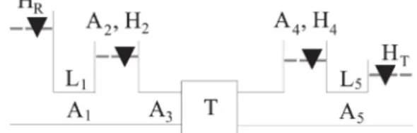
The scheme of this hydroelectric simulator including two surge tanks and the Francis hydraulic turbine considered in this work is recalled in Figure 3 [7]. As already remarked, but recalled here for the readers’ convenience, the hydroelec-tric simulator includes a reservoir with water level HR, an upstream water tun-nel with cross-section area A1 and length L1, an upstream surge tank with

cross-section area A2 and water level H2 of appropriate dimensions. A

down-stream surge tank with cross-section area A4 and water level H4 follows,

ending with a downstream tail water tunnel of cross-section area A5 and length 5

L . Moreover, between the Francis hydraulic turbine and the two surge tanks, there is a the penstock with cross-section area A3 and length L3. Finally,

Figure 3 highlights a tail water lake with level HT. The levels HR and HT of the reservoir and the lake water, respectively, are assumed to be constants.

The hydraulic system considered in this paper was modified by the authors in order to include the Francis hydraulic turbine, as presented in [7]. By consider-ing a pressure water supply system, the expressions of the Newton’s second law for a fluid element inside a pipe and the conservation mass law for a control vo-lume can be derived, which take into account the water compressibility and the pipe elasticity. If the penstock is assumed to be relatively short, the water and pipelines are considered incompressible. In this condition, only the inelastic wa-ter hammer effect needs to be considered. Therefore, the simplified and general relation of the penstock has the form of Equation (7):

w f

h _{T s H}

q = − −

(7) Moreover, Equation (7) represents the transfer function between the flow rate deviation and the water pressure deviation valid for a simple penstock. The va-riable h represents the water pressure relative deviation, whilst q is the flow rate relative deviation. The term Hf represents the hydraulic loss, with s the Lap-lace operator, and Tw the water inertia time expressed by the relation of Equa-tion (8): r w r LQ T gAH = (8) Note that the time variable Tw of the water inertia described by the relation of Equation (8) is a function of the hydraulic variable, such as the penstock length L, the rated flow rate Qr, the gravity acceleration g, the cross-section area

Figure 3. Overall scheme of the hydroelectric process.

A, and the rated water pressure Hr. The classic plant represented in Figure 3 can be separated into 3 subsystems, and namely the upstream water tunnel, the penstock, and the downstream tail water tunnel. The transfer functions between the flow rate deviation and water pressure deviation transfer functions of the three subsystems are summarised below. In this hydraulic system, the upstream water tunnel is connected with the reservoir and together with the upstream surge tank. Moreover, taking into account that the upstream water tunnel inlet coincides with the reservoir, and due to the constant value of the inlet water pressure deviation during hydraulic transients, the transfer function between the flow rate and the water pressure deviations of the upstream water tunnel outlet has the form of Equation (9):

1 1

1

1 w f

h _{T s H}

q = − − (9) On the other hand, the downstream tail water tunnel connects the down-stream surge tank with the tail water lake. The downdown-stream tail water tunnel outlet is assumed to coincide with the tailwater lake, with constant outlet water pressure deviation. In this way, the transfer function between the flow rate and the water pressure deviations of the downstream tail water tunnel inlet is represented in the form of Equation (10):

5 5

5

5 w f

h _{T s H}

q = − − (10) Usually, the draft tube water inertia is considered within the penstock. There-fore, the transfer function between the flow rate and the water pressure devia-tions within the penstock are expressed by the relation of Equation (11):

2 4 3 t h h h h= − + ₍₁₁₎ with: 3 3 3 3 w f h _{T s H} q = − − (12) The relations describing the surge tanks are formulated from the flow conti-nuity at the two junctions, by neglecting the hydraulic losses at surge tank ori-fices, and represented via the relations of Equations (13):

2 2 2 1 3 4 4 4 3 5 d d d d r r r r A H h _{q q q} Q t A H h _{q q q} Q t  _{= = −}    _{= = −}  (13) In this situation, the surge tank filling time has the form of Equation (14):

r s r AH T Q =

(14) The mathematical model and the performance curves of the Francis turbine considered in this work were obtained in order to describe the dynamic beha-viour of a realistic hydroelectric process. To this aim, the values of the most im-DOI: 10.4236/jpee.2019.71003 37 Journal of Power and Energy Engineering

portant variables the hydraulic system and the Francis hydraulic turbine, which represent the overall hydroelectric process simulator working at rated conditions are summarised in Table 2.

Note that, with reference to the values summarised in Table 2, the mathemat-ical description of the pure hydraulic system, which does not include the Francis hydraulic turbine, was proposed earlier in [16] and later in [17]. This model was modified by the authors and presented for the first time in [7]. The considered process includes a hydraulic turbine [15], whose performance curves and para-meters were selected in order to describe the dynamic behaviour of a realistic hydroelectric process [18].

After these considerations, in the following the procedure for computing the non-dimensional performance curves of the hydraulic turbine considered in this work is briefly recalled. In particular, the non-dimensional water flow rate

r

Q Q is expressed as a function of the non-dimensional rotational speed n nr, and represented by the second order polynomial of Equation (15):

(

)

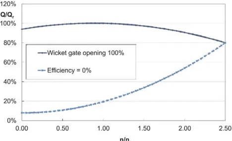
2 1 1 1 1 , r r r Q _{G a} n _b n _{c f n G} Q n n  _{   }    = _{ } + _{ }+ =         (15)

Moreover, the relation of Equation (15) includes the wicked gate opening, de-scribed by the non-dimensional parameter G, varying from 0 to 100%. In partic-ular, Figure 4 represents the curve derived for G =100%, i.e. fully open wicked gate. Moreover, the curve at

η =

0%

is also depicted, thus defining the operat-ing conditions of the Francis hydraulic turbine. Furthermore, the same poly-nomial curve of Equation (15) allows the computation of the water flow rate Q

as a function of the hydraulic turbine rotational speed n and its wicked gate opening G for all working conditions.

The hydroelectric simulator assumes that the turbine efficiency is constant and equal to its rated value ηr, i.e. 0.9, as reported in Table 2. Note that the hy-droelectric simulator does not include possible efficiency variation with the elec-tric load, even if the turbine efficiency ηr could be a function of the non-dimensional rotational speed n nr .

On the other hand, the non-dimensional turbine torque M results a function of the water flow rate Q, the water level H and the rotational speed n, as Table 2. Values of the main parameters of the hydroelectric plant simulator.

Variable Description Value

r

H Reservoir water level 400 m

r

Q Water flow rate 36.13 m3_/s

r

P Hydraulic turbine power 127.6 MW

r

n Turbine rated rotational speed 500 rpm

r

η Efficiency rated value 0.90

r

M Turbine-rated torque 2437 kNm

Figure 4. Representation of the non-dimensional water flow rate Q Qr with respect to

the non-dimensional rotational speed n nr. highlighted by the relation of Equation (16):

(

)

2 , , r r r r Q H Q H M _{f Q n G} n M n = = (16) Moreover, the combination of the relations of Equations (15) and (16) high-lights that the turbine torque M is a function of the water flow rate Q, the rota-tional speed n and wicked gate opening G.

Finally, the overall model of the hydroelectric simulator is described by the relations of Equations (17)-(20), which express the non-dimensional variables with respect to their relative deviations:

1 t r Q _q Q = + (17) 1 t r H _h H = + (18) 1 r n _x n = + (19)

1

G

= +

y

(20) with qt is the turbine flow rate relative deviation, ht the turbine water pres-sure relative deviation, x the turbine speed relative deviation, and y the wicket gate servomotor stroke relative deviation. Moreover, the relation of Equation (20) allows only negative values of y.

On the other hand, when the generator unit and its network are considered, and in particular the generator unit is connected only to an isolated load, the load characteristic of the generator unit is described by the dynamic model of Equation (21):

0 1 t g a g x m m− =T s e+

(21) with mg0 being the load torque, Ta representing the generator unit mechani-cal time, whilst the parameter eg is the load self-regulation factor. The va-riables and parameters of the hydroelectric model were selected according to the work [17] in order to represent a realistic hydroelectric plant simulator. Moreo-ver, as for the wind turbine benchmark, the signals that can be acquired from the actuator and sensors of the hydroelectric plant are modelled as the sum of the actual variables and stochastic noises, as proposed for the wind turbine bench-mark.

With reference to the control strategies for classic hydroelectric plants, stan-dard PID regulators are used to compensate the hydraulic turbine speed. There-fore, the actuated signal u is computed as sum of the proportional, integral, and differential terms of the error x in Equation (19), expressed in the form of Equa-tion (22): 1 i d p n K K s u x K s T s   =  + + ₊   

(22)

with Kp being the proportional gain, Ki the integral gain, and Kd the de-rivative gain. Tn is the parameter of the derivative filter time constant. The hy-droelectric simulator considered in this work exploits an electric servomotor that is used as a governor.

The servomechanism implemented in the hydroelectric simulator is described as a first-order model, which relates the control signal u with the wicket gate servomotor stroke y according to Equation (23):

1 1 y

y

u T s= ₊ (23)

with Ty representing the wicket gate servomotor response time.

This concludes the description of the complete nonlinear simulator of a typi-cal hydroelectric plant consisting of two surge tanks and a Francis hydraulic tur-bine, as represented in Figure 3.

Finally, it is worth noting that some relations of the hydroelectric system have been linearised, see e.g. Equations (7) and (17). However, this simplified model has been considered for comparison purpose, as the nonlinear parts of the processes under investigation are closer, as highlighted by Equations (1) and (15).

3. Data-Driven and Model-Based Control Methodologies

This section recalls the self-tuning control methodologies that will be designed and compared when applied to the considered energy conversion benchmark and simulator.

In general, control systems exploit design algorithms that force a dynamic model to track prescribed references or set-point, such that fixed objectives or DOI: 10.4236/jpee.2019.71003 40 Journal of Power and Energy Engineering

behaviour modes are achieved. In this way, the classic control problem is for-mulated as tracking task, where the system output has to follow the set-point, thus representing the final objective. Tasks expressed in this form are also present in energy conversion applications, for example the speed control of both wind and hydraulic turbines. However, it could be useful to improve the prob-lem descriptions and to give a deeper insight into possible solutions, in order to achieve all potentials of control theory when applied to energy conversion sys-tems.

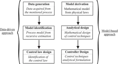
Figure 5 highlights the main differences between the proposed data-driven and model-based approaches to the design of the control solutions.

On one hand, data-driven techniques rely on the availability of the in-put-output data acquired from the monitored plant. These data are use for the on-line estimation of a suitable model of the dynamic process, which is thus ex-ploited for the identification of the control law to be applied to the controlled system. On the other hand, model-based methods require the mathematical de-scription of the monitored plant, in the form of input-output or state-space re-presentations. These forms are thus employed for the analytical derivation of the mathematical function of the controller, again in form of input-output or state-space relations. Both the derived controllers are obtained in order to reach prescribed performances.

First, with reference to the process output, the desired transient or steady-state responses can be considered, as for the case of self-tuning PID regu-lators summarised in Section 3.1. On the other hand, if the frequency behaviour is taken into account, the desired closed-loop poles can be fixed as roots of the closed-loop transfer function. This represents the design approach used by the adaptive strategy considered in Section 3.3. Moreover, when robust perfor-mances are included, the minimisation of the sensitivity of the closed-loop sys-tem with respect to the model-reality mismatch or external disturbances can be considered. This approach is related for example to the fuzzy logic methodology

Figure 5. Key aspects of data-driven and model-based approaches.

reported in Section 3.2. Some other strategies provide solutions to this optimisa-tion problem when it is defined at each time step, as for the case of the Model Predictive Control (MPC) with disturbance decoupling considered in Section 3.4. The considered strategy integrates the advantages of the MPC solution with the disturbance compensation feature.

It is worth noting that model-based control designs rely on the mathematical descriptions of the process models, in order to derive the control laws. The de-sign of standard PID regulators and Model Predictive Control (MPC) methods follows a model-based approach, which will be illustrated in Sections 3.1 and 3.4, respectively. However, the need for these high-fidelity mathematical descriptions can require much more effort than the derivation of the controller models. Therefore, dynamic system identification methodologies have been successfully proposed in order to determine the so-called black-box representations, which is also used for the self-tuning PID design. Usually, these descriptions do not present structural relationships to the physical processes. On the other hand, dynamic system identification schemes can be also exploited for deriving adap-tive controller prototypes, which are thus able to adapt themselves with respect to unknown conditions or time-varying systems. By means of this “self-tuning mode”, adaptive control strategies relying on linear models of the controlled process are also able to track changes of the plant. Examples of these data-driven approaches are represented by the fuzzy logic and adaptive controllers recalled in Sections 3.2 and 3.3, respectively. On the other hand, the MPC strategy ex-ploits the proposed disturbance compensation method, which is thus able to cope with uncertainty and model-reality mismatch effects.

In general, the mathematical formulation of the control law can be provided as linear or nonlinear dynamic function  in the form of Equation (24):

( )

(

( )

)

u t =  y t (24) with y t

( )

being the monitored output, whilst u t

( )

is the control input. The control techniques proposed for the systems under investigation should lead to the computation of the control law of Equation (24) generating the input u t

( )

that allows to track the given reference or set-point r t

( )

for the controlled output y t

( )

.

3.1. Autotuning Model-Based PID Control

Industrial processes commonly exploit closed-loop including standard PID con-trollers, due to their simple structure and parameter tuning [19]. The control law depends on the tracking error e t

( )

defined by the difference between the de-sired and the measured output signals, i.e. e t

( ) ( ) ( )

=r t −x t _{. This signal is} in-jected into the controlled process after proportional, integral and derivative computations. Therefore, the continuous-time control signal u t

( )

is generated by the PID regulator in the form of Equation (25):

( )

( )

₀

( )

d d

( )

d t p i d e t u t K e t K e K t τ τ = +

_∫

+

(25) DOI: 10.4236/jpee.2019.71003 42 Journal of Power and Energy Engineering

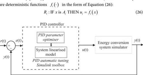
with Kp, Ki, Kd being the PID proportional, integral, and derivative gains, respectively. The most common strategy exploited for the computation of the optimal parameters of the PID governor uses proper Ziegler-Nichols formulas, as described in [19]. However, with the development of relatively recent auto-matic software routines, the PID optimal parameters can be easily determined by means of direct tuning algorithms implemented for example in the Simulink en-vironment. These strategies require the definition of the controlled process as Simulink model, such that they balance the input-output performances of the monitored system in terms of response time and stability margins (robustness) [19]. In particular, the PID automatic tuning procedure implemented in the Si-mulink toolbox performs the computation of the linearised model of the energy conversion systems studied in this paper. The logic scheme of this procedure is sketched in Figure 6.

Note finally that the PID block in Figure 6 performs the computation of a li-nearised model of the controlled system, if required. Therefore, the optimiser in-cluded in the PID block and implemented in the Simulink environment derives of the PID parameters that minimise suitable performance indices [19].

3.2. Data-Driven Fuzzy Logic Control

Fuzzy Logic Control (FLC) solutions are often exploited when the dynamics of the monitored process are uncertain and can present nonlinear characteristics. The design method proposed in this work exploits the direct identification of rule-based Takagi-Sugeno (TS) fuzzy prototypes. Moreover, the fuzzy model structure, i.e. the number of rules, the antecedents, the consequents and the fuzzy membership functions can be estimated by means of the Adaptive Neu-ro-Fuzzy Inference System (ANFIS) toolbox implemented in the Simulink envi-ronment [20]. The authors already suggested to employ regulators in the form of TS fuzzy models for designing fault diagnosis and fault tolerant control strate-gies presented e.g. in [21].

The TS fuzzy prototype relies on a number of rules Ri, whose consequents are deterministic functions f ⋅i

( )

in the form of Equation (26):

( )

: IF is THEN

i i i i

R x A u = f x

(26)

Figure 6. Block diagram of the monitored system controlled by the PID regulator with automatic tuning.

where the index i=1, 2, ,_ K _{describes the number of rules} K_, x _{is the input}

vector containing the antecedent variables, i.e. the model inputs, whilst ui represents the consequent output. The fuzzy set Ai describing the antecedents in the i-th rule is described by its (multivariable) membership function

( )

[ ]

0,1

i

A x

µ

→ _{. The relation} f x_i

_{( )}

assumes the form of parametric affine model represented by the i-th relation of Equation (27):

T

i i i

u a x b= + ₍₂₇₎

with the vector ai and the scalar bi being the i-th submodel parameters. The vector x consists of a proper number n of delayed samples of input and output signals acquired from the monitored process. Therefore, the term T

i

a x is an Auto-Regressive eXogenous (ARX) parametric dynamic model of order n, and

i

b a bias.

The output u of the TS fuzzy prototype is computed as weighted average of all rule outputs ui in the form of Equation (28):

( ) ( )

( )

1 1 i i K A i i K A i x y x u x µ µ = = =

∑

∑

(28) The estimation scheme implemented by the ANFIS tool follows the classic dynamic system identification experiment. First, the structure of the TS fuzzy prototype is defined by selecting a suitable order n, the shape representing the membership functions µA_i, and the proper number of clusters K. Therefore, the input-output data sequences acquired from the monitored system are exploited by ANFIS for estimating the TS model parameters and its rules Ri after the se-lection of a suitable error criterion. The optimal values of the controller parame-ters represented by the variables ai and bi of (27) are thus estimated [22].

The work proposes also a strategy different from ANFIS that can be exploited for the estimation of the parameters of the fuzzy controller. This method relies on the Fuzzy Modelling and Identification (FMID) toolbox designed in the Mat-lab and Simulink environments as described in [23]. Again, the computation of the controller model is performed by estimating the rule-based fuzzy system in the form of Equation (28) from the input-output data acquired from the process under investigation. In particular, the FMID tool uses the Gustafson-Kessel (GK) clustering method [23] to perform a partition of input-output data into a proper number K of regions where the local affine relations of Equation (27) are valid. Also in this case, the fuzzy controller model of Equation (28) is computed after the selection of the model order n and the number of clusters K. The FMID toolbox derives the variables ai and bi, as well as the identification of the shape of the functions µA_i by minimising a given metric [23].

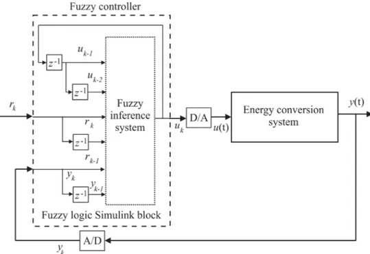
Note that the overall digital control scheme consisting of the discrete-time fuzzy regulator of Equation (28) and continuous-time nonlinear system of Equa-tion (24) includes also Digital-to-Analog (D/A) and Analog-to-Digital (A/D) converters, as shown in Figure 7.

With reference to Figure 7, note finally that the fuzzy controller block imple-mented in the Simulink environment includes a suitable number n of delayed samples of the signals acquired from the monitored process. Moreover, the fuzzy inference system in Figure 7 implements the TS model of Equation (28). The delay n, the membership functions µA_i, and the number of clusters K are esti-mated by the FMID and the ANFIS toolboxes, as described in [23].

3.3. Data-Driven Adaptive Control

The adaptive control technique proposed in this work relies on the recursive es-timation of a 2nd order discrete-time transfer function G z

( )

with time-varying parameters described by Equation (29):

( )

1 1 2 2 1 2 1 2 1 z z G z z z β β α α − − − − + = + + (29) where αi and βi are identified on-line at each sampling time tk =kT , with

1,2, ,

k

=

_

N

_{, for N samples, and T being the sampling interval.}

_z

−1 _indicates

the unit delay operator. A viable and direct way for deriving the model parame-ters in Equation (29) that is proposed in this work is based on the Recursive Least-Square Method (RLSM) with directional forgetting factor, which was pre-sented in [24].

Once the parameters of the model of Equation (29) have been derived, this paper proposes to compute the adaptive controller in the form of Equation (30):

(

)

0 1 1 2 2 1 1 2

k k k k k k

u =q e q e+ − +q e− + −γ u − +γu −

₍₃₀₎

with ek and uk represent the sampled values of the tracking error e t

( )

and the control signal uk at the time tk, respectively. With reference to the description

Figure 7. Block diagram of the monitored system controlled by the fuzzy regulator.

of Equation (30), by following a modified Ziegler-Nichols criterion, q0, q1, q2,

and γ represent the adaptive controller parameters, which are derived by solving a Diophantine equation. As described in [24], by considering the recur-sive 2-nd order model of Equation (29), this technique leads to the relations of Equations (31):

(

)

0 1 1 1 1 2 1 2 2 1 1 1 1 2 1 2 2 1 2 1 1 ₁ 1 q d s r s q r s q r α γ β β γ α α β α β β α  = + − −    =    _{ }  = − _ − + _  _{ }   =  

(31) where:

(

)

(

)

(

)(

)

(

)

(

)

2 2 1 1 2 1 2 1 2 1 2 1 2 1 2 1 2 2 1 2 1 2 2 1 2 r b b a b b a b b s a b b a b a b b b d b d b  = + − −   = + − + − −  (32)

Note that the design technique proposed in this work and represented by the relations of Equations (31) and (32) assumes that the behaviour of the overall closed-loop system can be approximated by a 2nd _{order transfer function with}

characteristic polynomial represented by Equation (33):

( )

2 ₂ 2

D s = +s

δω ω

s+

(33) with δ and ω being the damping factor and natural frequency, respectively.

s is the derivative operator. Furthermore, if δ ≤1_{, the following relations are} used [24]:

(

2

)

1 2 2 2e cos 1 e T T d T d δω δω

ω

δ

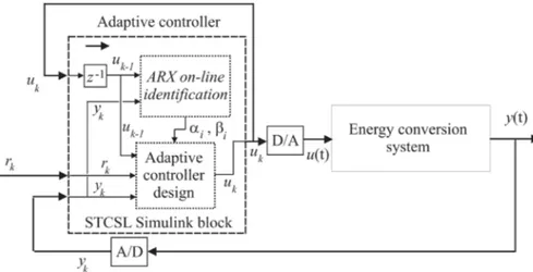
− −  = − −    =  (34) This paper suggested this adaptive control technique since both the recursive estimation procedure of Equation (29) and the on-line computation of the con-trol law of Equation (30) are available from the digital Self-Tuning Concon-troller Simulink Library (STCSL) described in [24]. According to this solution, the output yk of the time-varying model of Equation (29) follows the reference signal rk when the control law of Equation (30) is. The achievable perfor-mances depend on the design parameters given by Equation (33).

The on-line control law of Equation (30) is used for the regulation of the con-tinuous-time nonlinear system of Equation (24) by including D/A and A/D converters, as highlighted in the scheme of Figure 8.

Note finally that the adaptive control sketched in Figure 8 is implemented via the STCSL block in the Simulink environment. It includes the module perform-ing the on-line identification of the ARX model of Equation (29), which is used for the adaptive controller design in the form of Equation (30).

3.4. MPC with Disturbance Decoupling

The general structure of the proposed MPC is illustrated in Figure 9, with the MPC managing objectives and constraints of the control inputs. The MPC works as a standard MPC controller when the nominal plant is considered, and gene-rates the reference inputs. In the presence of disturbance or uncertainty effects, the considered solution provides the reconstruction of the equivalent distur-bance signal acting on the plant. This represents the key feature of this structure, which compensates the disturbance effect and “hide” it to the overall system. In this way, it decouples the disturbance effect from the nominal MPC design. Another feature of this structure is the management of the objectives and con-straints through the MPC design. These objective and concon-straints can be the nominal ones. But in case of disturbance or uncertainty, when the nominal per-formance cannot be achieved, the objectives could be switched to degraded ones and the constraints can also be updated if necessary. The powerful tool to achieve the required fault tolerance characteristic is the optimisation lying in the

Figure 8. Block diagram of the monitored system controlled by the adaptive regulator.

Figure 9. Block diagram of the monitored system controlled via the disturbance com-pensated MPC scheme.

MPC design itself.

The overall scheme is thus represented aim by the MPC design with distur-bance compensation, such that the compensated system has response very simi-lar to the nominal system and the constraints are not violated. The fault com-pensation problem within the MPC framework is defined as follows. Given a state-space representation of the considered system affected by disturbance or uncertainty has the following form:

l l l l d l l l x A x B u B d w y C x v = + + +   = +   (35) and its nominal reference model:

r l r l r r l r x A x B u y C x = +   =   (36) the disturbance compensation problem is solved by finding the control input u

that minimises the cost function:

(

2 2

)

_d

c t N t l r Q R t

J

=

_∫

+ ∆

x x

−

+

u



τ

(37) given the reference input ur.

In Equation (35) the matrices Al, Bl, Bd and Cl are of proper dimen-sions. The vector yl represents the output measurements, xl is the state of the model with disturbance, whilst xr is the reference state, and yr the refer-ence output, corresponding to the referrefer-ence input ur of the nominal model. The vectors w and v include the model mismatch and the measurement error, respectively. d represents the equivalent disturbance signal. In Equation (37) t is the current time, t∆ _{is the control interval, and} N_c is the length of the control horizon. Q and R are suitable weighting matrices. Note that the model of Equa-tion (35) can be derived by nonlinear model linearisaEqua-tion or identificaEqua-tion pro-cedures, as suggested in Sections 3.1 and 3.3, respectively.

This work proposes to solve the problem in two steps: the reconstruction of the disturbance d, i.e. ˆd, provided by the disturbance estimation module, and the MPC tool. Due to the model-reality mismatch and the measurement error in (35), the Kalman filter (38) is used to provide the estimation of the state vector

l

x , the output yl of the system affected by the estimated disturbance ˆd:

(

)

ˆ l l l l l f l l l l l l x A x B u B d K y C x y C x  = + − + −   =   (38) where Kf is the Kalman filter gain. In this way, based on the estimations ˆd and xl, an MPC is designed, which contains the reference model of Equation (36) and the filtered system of Equation (38), with ˆd provided by the Kalman filter. Moreover, the MPC has the objective function:

(

) (

T

)

T

_d

c t N t l r l r t

x x Q x x

u Ru τ

+ ∆

_

_

−

−

+





∫

 

(39) in which xl and xr are the states of the filtered and the reference models, re-spectively. The integrated MPC with the Kalman filter solves this general dis-DOI: 10.4236/jpee.2019.71003 48 Journal of Power and Energy Engineering

turbance compensation problem, as long as the estimations of both the state and the disturbance are correct. An illustration of the structure of the fault compen-sated MPC is shown in Figure 9.

The global estimation and control scheme is a nonlinear MPC problem with the nominal model for the considered energy conversion systems of Equation (35), the disturbance d with its estimator, and the Kalman filter of Equation (38) as prediction model. The local observability of the model of Equation (35) is es-sential for state estimation, which is easily verified. The implementation of the proposed disturbance compensation strategy has been integrated into the MPC Toolbox of the Simulink environment.

4. Simulation Results and Comparisons

This section presents the simulations achieved in the Matlab and Simulink envi-ronments implementing the control techniques and tools recalled in Section 3. The obtained results are evaluated via the percent Normalised Sum of Squared Error (NSSE%) performance function in the form of Equation (40):

(

)

2 1 2 1 % 100 N k k k N k k r o NSSE r = = − =

∑

∑

(40) with rk being the sampled reference or set-point r t

( )

, whilst ok is the sam-pled continuous-time signal representing the generic controlled output y t

( )

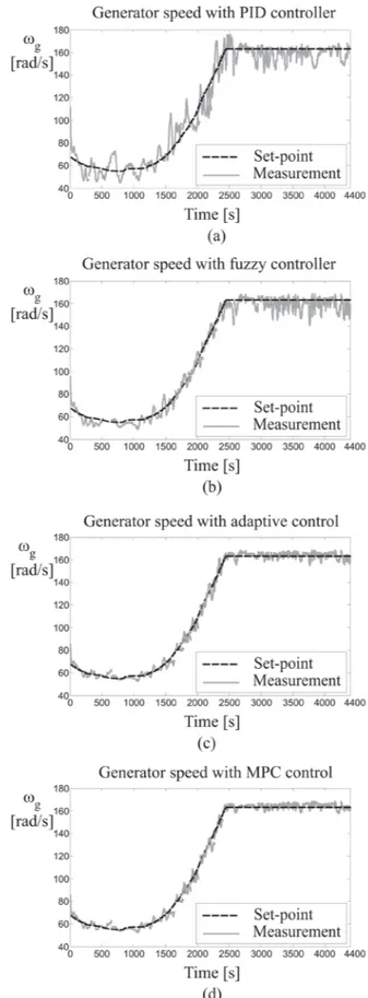
of the process. In particular, this signal is represented by the wind turbine genera-tor angular velocity ωg

( )

t in Equation (3), and the hydraulic turbine rotational speed n in Equation (19) for the hydroelectric plant.

Note that the wind turbine benchmark and the hydroelectric plant simulator of Section 2 allow the generation of several input-output data sequences due to dif-ferent wind speed v t

( )

effects (see e.g. (1)) and hydraulic transient under varia-ble loads mg0 (see e.g. (21)), respectively. Moreover, in order to obtain

compara-ble working situations, the wind turbine benchmark has been operating from par-tial to full load conditions, as highlighted in Figure 2(b). It is thus considered the similar maneuver of the hydroelectric system operating from the start-up to full load working condition. After these considerations, Section 4.1 summarises the results obtained from the wind turbine benchmark first. Then, the same control techniques will be verified when applied to the hydroelectric simulator.

It is worth highlighting that the simulations considered in this work take into account disturbance and uncertainty effects. In fact, the hydroelectric plant con-siders a load disturbance, whilst the turbine simulator is driven by wind, which represents the main disturbance source. Moreover, the uncertainty effect has been analysed in Section 4.2.

4.1. Control Technique Performances and Comparisons

Figure 10 reports the results achieved with the control methodologies and the DOI: 10.4236/jpee.2019.71003 49 Journal of Power and Energy Engineering

tools summarised in Section 3. In particular, Figure 10 depicts the wind turbine generator angular velocity ωg when the wind speed v t

( )

changes from 3 m/s to 18 m/s for a simulation time of 4400 s. This simulation time is defined by the wind turbine benchmark in [9] using a real wind sequence sampled for 4400 s. Moreover, the initial value of the signal ωg is different from zero since the si-mulation commences when the wind speed has already exceeded the cut-in value highlighted in Figure 2(b).

In detail, with reference to the picture in Figure 10(a), the parameters of the PID regulator of Equation (25) have been determined using the model-based autotuning tool available in the Matlab and Simulink environments. They were settled to K =p 4.0234, K =i 1.0236, K =d 0.0127, as described in Section 3.1. The achieved performances are better than the ones obtained with the baseline control laws proposed in [9] and recalled in Section 2.1.

Moreover, Figure 10(b) shows the simulations achieved with the data-driven fuzzy identification approach recalled in Section 3.2. This strategy was proposed here since it represents a viable and practical way for deriving the models of the controllers by means of the so-called model reference control approach, as ad-dressed in [25]. According to this strategy, the baseline PID regulators designed for the nominal wind turbine model were considered as reference controllers for the generation of the input-output data used by the identification methodology recalled in Section 3.2. In this way, the TS fuzzy controller parameters are esti-mated such that they optimise the performances in terms of tracking error. In particular, a sampling interval

T =

0.01s

has been exploited, and the TS fuzzy controller of Equation (28) has been obtained for a number K =3 of Gaussian membership functions, and a number n =2 of delayed inputs and output. The antecedent vector in Equation (27) is thus

[

k, k1, k 2, k 1, k 2

]

x= e e− e− u − u − . Both the data-driven FMID and ANFIS tools

availa-ble in the Matlab and Simulink environments provide also the optimal identifi-cation of the shapes of the fuzzy membership functions µA_i of the fuzzy sets

i

A in Equation (26).

On the other hand, the picture in Figure 10(c) shows the capabilities of the adaptive controller of Equation (30). The time-varying parameters of this da-ta-driven control technique summarised in Section 3.3 have been computed on-line via the relations of Equations (31) with the damping factor and the nat-ural frequency variables δ ω= =1 _{in Equation (33). As already remarked, this} work considered this data-driven adaptive technique since it was already imple-mented in the Simulink environment via the Self Tuning Controller Simulink Library (STCSL) [24].

Finally, the picture of Figure 10(d) highlights the results achieved with the MPC technique with disturbance decoupling recalled in Section 3.4. The state-space model of the wind turbine nonlinear system of Equation (3) ex-ploited for the design of the MPC and the Kalman filter for the estimation of the disturbance has order n =5, with a prediction horizon N =p 10 and a control DOI: 10.4236/jpee.2019.71003 50 Journal of Power and Energy Engineering

Figure 10. Wind turbine controlled output compensated by (a) the autotuning PID regu-lator, (b) the fuzzy controller, (c) the adaptive reguregu-lator, and (d) the MPC approach with disturbance decoupling.

horizon N =c 2. The weighting factors have been settled to w =yk 0.1 and

1

k

u

w = , in order to reduce possible abrupt changes of the control input. Note that, in this case, the MPC technique has led to the best results, since it exploits a disturbance decoupling strategy, whilst its parameters have been iteratively adapted in the Simulink environment in order to optimise the MPC cost func-tion of Equafunc-tion (37), as addressed in Secfunc-tion 3.4.

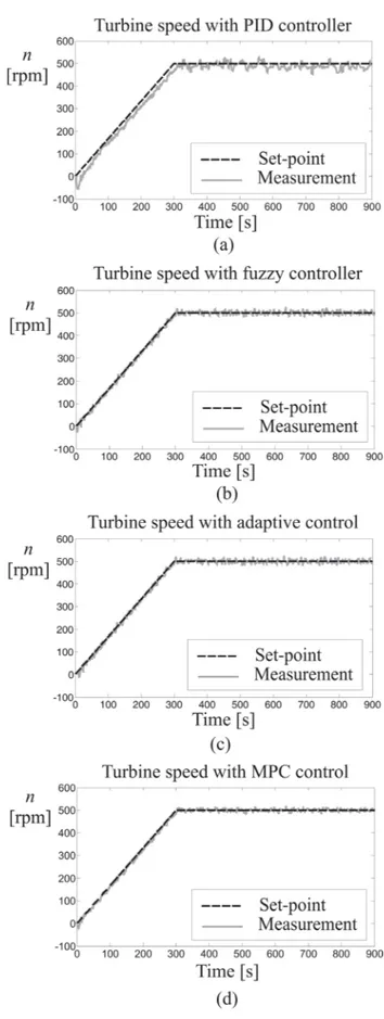
The second test case regards the hydroelectric plant simulator, where the hy-draulic system with its turbine speed governor generates hyhy-draulic transients due to the load changes. As already recalled in Section 2.2, an effective behaviour of a classic PID governor addressed e.g. in [17] applied to this hydroelectric plant would require the scheduling of its gains. In such a way only the perfor-mance of this standard controller could have been improved. In fact, in order to obtain the best dynamic performance of the hydraulic turbine, the PID governor of the turbine speed in Equation (22) should consider different parameters for each working condition. Therefore, in order to consider operating situations similar to the wind turbine benchmark, the capabilities of the considered control techniques applied to the hydroelectric simulator have been evaluated during the start-up to full load maneuver. Moreover, an increasing load torque mg0 in

Equation (21) has been imposed during the start-up to full load phase, which is assumed to last 300 s because of the large size of the considered Francis turbine, and for a simulation of 900 s. This represents one of the different working con-ditions already addressed by the authors in [21] but for fault diagnosis applica-tions. It is worth noting that these slow varying set-points have been considered for comparison purpose.

Under these assumptions, Figure 11 summarises the results achieved with the application of the control strategies recalled in Section 3. In particular, for all cases, Figure 11 highlights that the hydraulic turbine angular velocity n increas-es with the load torque mg0 during the start-up to full working condition

ma-neuver.

In more detail, Figure 11(a) shows the performance of the PID regulator when its parameters are determined via the model-based autotuning procedure recalled in Section 3.1. In particular, its gains are determined with the algorithm implemented in the Simulink environment. It tries to compute in an automatic way the optimal parameters of the PID regulator that minimise the step response tracking error of the linear model approximating the nonlinear behaviour of the hydraulic plant. Furthermore, Figure 11(a) shows that the PID governor with autotuning is able to keep the hydraulic turbine rotational speed error n n− r null (r t

( )

=nr, i.e. the rotational speed constant) in steady-state conditions.

Figure 11(b) reports the results concerning the TS fuzzy controller described by Equation (28) in Section 3.2. This fuzzy controller was implemented for a sampling interval

T =

0.1s

, with a number K =2 of Gaussian membership functions, and a number n =3 of delayed inputs and output. The antecedent vector exploited by the relation of Equation (27) is thus

Figure 11. Hydroelectric system with (a) the autotuning PID regulator, (b) the fuzzy controller, (c) the adaptive regulator, and (d) the MPC approach with disturbance de-coupling.