Multi-scale habitat suitability models for the Eurasian otter Lutra lutra

(1)

Università degli studi del Molise

Facoltà di Scienze Matematiche Fisiche e Naturali

MODELLI DI IDONEITA’ AMBIENTALI PER LA LONTRA

EUROASIATICA A DIVERSE SCALE

Multi – scale habitat suitability models for the Eurasian otter Lutra lutra (Mamalia, Carnivora, Mustelidae)

Tesi di dottorato in Ambiente e Territorio

Presentata alla

Facoltà di Scienze Matematiche Fisiche e Naturali

Da

Carmen Cianfrani

Tutor: Prof.ssa Anna Loy

Co-turor: Prof Antoine Guisan

(2)

Table of content

1. Introduction……….p. 5

1.1 Habitat suitability models - A tool for the conservation of the biodiversity…….p. 5 1.2 The otter – The situation in Europe and in Italy………...p. 13 1.3 Objectives and contents of the main chapters………...p. 16

2. Habitat suitability and connectivity for the otter………p. 18

3. Habitat suitability to predict the recovery of the otter………p. 35

4. Impacts of climate change on the European otter distribution………..p. 56

5. Perspectives………...p. 75

6. Conclusions………...p. 80

7. Acknowledgments………...p. 81

(3)

Summary

Durante gli ultimi cinquanta anni, l’areale europeo della lontra euroasiatica (Lutra lutra) si è drammaticamente ridotto. Attualmente la lontra sembra stia recuperando in alcuni paesi europei, ma alcune popolazioni sono ancora frammentate e la specie è tuttora quasi assente dall’ Europa centrale. In Italia la situazione è particolarmente critica, con un piccola popolazione che sopravvive nei bacini merdionali, a sua volta divisa in due nuclei isolati. Promuovere l’espansione delle popolazioni redisidue è di vitale importanza per assicurare il mantenimento della diversità genetica e la persistenza a lungo termine della specie. A questo proposito i modelli di idoneità ambientale (HSM) rappresentano potenti strumenti per valutare la qualità degli habitat e produrre carte di distribuzione potenziale e dispersione naturale della specie. Il progetto di ricerca ha avuto come obiettivo primario l’individuazione dei fattori che influenzano la distribuzione della lontra in Italia e la messa a punto di modelli in grado di predire la distribuzione potenziale della specie a diverse scale, regionale e europea.

Il modello a scala regionale riguarda il nucleo settentrionale dell’areale della lontra in Italia, principalmente costituito dalla regione Molise. Per quest’area è stato sviluppato un modello di idoneità ambientale deduttivo, basato sull’opinione degli esperti. Questo modello è stato utilizzato come base per effettuare un’analisi di connettività, longitudinale e laterale.

Nella stessa area di studio sono stati sviluppati modelli inferenziali per testare la capacità di individuare potenziali aree di espansione per la specie. Per testare la capacità di predizione dei modelli sono usati usati dati raccolti in due campagne di rilevamento, una effettuata prima della colonizzazione e l’altra dopo la ricolonizzazione. Sono stati utilizzati l’ENFA (Environmental Niche Factor Analysis) e il GLM (Generalised Linear Model). Il primo approccio utilizza solo i dati di presenza, il secondo anche quelli di assenza. I due modelli sono stati calibrati con dati raccolti prima della colonizzazione e poi con i dati raccolti sul fiume ricolonizzato. I modelli sono stati comparati e i modelli sviluppati con i dati pre-colonizzazione sono stati validati con i dati post-colonizzazione. Questo studio ha dimostrato che i dati di assenza in una situazione di instabilità tra la specie e le aree idonne occupate porta ad errori di predizione.

Nel modello a scala europea sono state considerate sia le condizioni climatiche attuali sia le predizioni relative ai cambiamenti climatici futuri. Nell’analisi sono state considerate le variabili ambientali che posso essere in relazione ai requisiti ecologici della specie, ovvero alla disponibilità di acqua, alla disponibilità di risorse trofiche, di siti di rifugio e al disturbo antropico. Gli scenari futuri sono stati ottenuti utilizzando i parametri disponibili relativi al raddoppio della CO2 nell’atmosfera (modello CCM3). I risultati hanno mostrato come a scala europea la distribuzione della lontra sia influenzata principalmente dalla disponibilità di acqua.

(4)

La distribuzione attuale potenziale mostra larghe aree di habitat non idonei nel centro Europa, che limitano la connettività tra le tre sub-popolazioni occidentale, orientale e italiana. Gli scenari futuri indicano una potenziale perdita di habitat idonei nelle regioni occidentali, mentre in Europa centrale e orientale il modello predice un incremento. Le previsioni future indicano anche una diversa localizzazione dei corridoi di habitat che potrebbero favorire l’espansione e il collegamento delle popolazioni. Il modello è stato quindi integrato con i dati relativi alle aree protette. Il confronto ha permesso di individuare le aree più critiche che attualmente e in futuro dovranno essere preservate per garantire la sopravvivenza e il flusso genico delle popolazioni di lontra in Europa.

(5)

CHAPTER 1 - INTRODUCTION

1.1 Habitat suitability models - A tool for the conservation of the

biodiversity

Habitat suitability models (HSMs) are empirical models relating field observations to environmental predictor variables based on statistically or theoretically derived response surfaces (Guisan and Thuiller, 2005, Fig. 1). By integrating known occurrences of species with environmental GIS layers that summarize meaningful niche dimensions, it is possible to determine the key combinations of environmental conditions enabling a species to grow and reproduce.

HSMs take advantage of revolutionary advances in the field of geographical information systems (GIS) and biodiversity informatics (Graham et al., 2004; Kozak,) which result in the higher availability and quality of two major sources of data:

1) Environmental predictors, including global coverage of digital terrain, climate, soil, and land-cover surfaces are now available at relatively fine spatial resolution (mostly 1km grid), thank to recent advances in interpolating climatic data from meteorological stations and remote sensing technologies. Environmental predictors can exert direct or indirect effects on species (Austin, 2002), and are optimally chosen to reflect the three main type of influences on the species: (i) limiting factors (or regulators) defined as factors controlling species eco-physiology (e.g. temperature, water, soil composition); (ii) disturbances, defined as all type of perturbations affecting environmental systems (natural or human-induced) and (iii) resources, defined as all compounds that can be assimilated by organisms (e.g. energy and water).

2) Species data sets from biological surveys and natural history collections. Species data can be simple presence, presence-absence or abundance observations based on random or stratified field sampling, or observation obtained opportunistically, such as those in natural history collection (Graham et al., 2004). The accessibility of such data is improving dramatically as a result of rapid advances in the digitization of museum and herbarium specimen collections which contain the locations of observation or collection for large numbers of species across a wide range of higher taxa (Bisby, 2000; Graham et al., 2004).

(6)

Fig. 1 – Schematic representation illustrating the main steps of habitat suitability modelling. The distribution of the species data are shown on geographical and environmental spaces. The presences (squared) and absences (crosses) data are linked to environmental predictors in a geographical information system (GIS) and environmental values are attributed to them. Statistical response surfaces are then derived in the environmental space and predicted back to the geographical space to build a potential distribution map. The predictions on the map indicate the probability of presence of the species in each regions of the study area.

Today, an impressive diversity of modelling techniques are available for modelling species distribution (see Guisan & Thuiller, 2005, tab. 2), depending on the type of response variable and predictors at hand. The choice of statistical method in a specific modelling context is now supported by many published comparison (Elith et al., 2006; Elith & Graham, 2009). These modelling techniques usually include an algorithm to select the most influential predictor in the model (Johnson & Omland, 2004). The most popular – but also controversial – technique consists in the stepwise selection procedure (see Guisan et al., 2002). Starting with a full model including all the variables, variables are sequentially introduced and removed in the model. At each step, predefined rules such as deviance reduction inform to keep or remove the specific predictor.

HSMs are useful if they are robust. Addressing ecological questions with a model that is statistically significant but only explains a low proportion of variance might lead to weak, possibly erroneous, conclusions (Mac Nally, 2002). Similar problems may well arise in the opposite case, when a model is over-fitted. Even though no absolute measure of

(7)

robustness of a model exists (Araujo et al., 2005), techniques for statistically evaluating models and their predictions are available and have considerably improved in many way (Fielding & Bell 1997, Pearce & Ferrier, 2000, see also Box 2).

Tool Reference Method implemented

BIOCLIM Busby 1991 CE

ANUCLIM See BIOCLIM CE

BAYES Aspinall 1992 BA

BIOMAPPER Hirzel et al 2002 ENFA

BIOMOD Thuiller 2003a GLM, GAM, CART, ANN, BRT, RF, MDA, MARS

DIVA Hijmans et al 2001 CE

DOMAIN Carpenter et al 1993 CE

ECOSPAT Unpublished data GLM, GAM

GARP Stockwell & Peters 1999 GA (incl. CE, GLM, ANN)

GDM Ferrier 2002 GDM

GRASP Lehmann et al. 2002b GLM, GAM

MAXENT Phillips et al. 2006 ME

SPECIES Pearson et al. 2002 ANN

Tab. 1 – Published predicted NBM packages, reference paper, related modelling methods. ANN, artificial neural networks; BA, Bayesian approach; BRT, boosted regression trees; CE, climatic envelop; CART, classification and regression trees; ENFA ecological niche factor analysis; GA, genetic algorithm; GAM generalised additive model; GDM, generalized dissimilarity modelling; GLM, generalized linear models; ME, maximum entropy; MDA, multiple discriminant analysis; MARS, multiple adaptive regression splines; RF, random forest. From Guisan & Thuiller 2005.

The calibration of HSMs should be proceed by an initial conceptual phase, which consist in defining an up-to-date conceptual model of the system to be simulated based on sound ecological thinking and clearly defined objectives (Austin, 2002). Notably, a special attention must be drawn on the setting of working hypotheses (e.g. pseudo-equilibrium; Guisan & Thiller 2005), the assessment of available and missing occurrence data, the relevance of environmental predictors for the focal species and the given scale and choice of the appropriate spatio-temporal resolution and geographic extent for the study. These aspects have been reviewed in a recent paper by Guisan and Thuiller (2005).

Lacks of consideration in these aspects can be potentially leading to:

i) Poor predictive ability (e.g. due to taxonomic and geographic biases, missing of relevance of environmental predictors at particular scale or missing availability of absence data).

(8)

ii) Consistent over- or under-optimism in predictions with new data (e.g. due to spatial autocorrelation, wrong choice of the modelling technique, small samplings).

iii) Apparent responses to environmental conditions inconsistent with biological understanding (e.g. due to spatial autocorrelation, small sampling, spurious response curves on incompletely sampled gradient.

Niche based models relying on data from natural history collection contribute significantly to conservation efforts that are directed toward species of concern, multi-species

Conservation prioritization schemes of the spread of the endangered species and predictions of biodiversity consequences of climate change (Coetzee et al., 2009).. HSMs techniques thus offer unique opportunities to track distributional changes in relation to threatening processes and thereby anticipate future impacts.

The choice of the appropriate scale in HSMs

A central and recurrent issue in HSMs building is identifying the appropriate scale for modelling. Scale is usually best expressed independently as resolution (grain size) and extent of the study area, because modelling a large area does not necessarily imply considering a coarse resolution. No question in spatial ecology can be answered without referring explicitly to these components at which data are measured or analysed. A first possible mismatch can occur between the resolution at which species data were sampled (e.g. plot size in field surveys, grid size in atlas surveys) and the one at which environmental predictors are available. Optimally, both should be the same, but such coherence is not always possible. For instance, the minimum resolution for GIS data might be too large to realistically allow an exhaustive field sampling of biological features to be conducted in the field, and thus smaller sampling units may need to be defined within larger modelling units or at the intersection of grids. Furthermore, many environmental data are indeed provided in a grid lattice format – i.e. regular point data – rather than a true raster format, which complicates the story, somewhat. This is for instance the case of many digital elevation models (DEM) and derived data (e.g. topographic and interpolated climatic maps). Indeed, designing field sampling in order to match raster units will work well in the case of true rasters (e.g. satellite images and derived products, such as CORINE land-cover), whereas placing sampling plots at intersections of a grid may prove more appropriate in the case of lattice grids. The problem then is to combine these different types of data in a single model. Aggregating these to a coarser resolution can sometimes

(9)

provide a simple yet efficient solution, as for instance allowing passing from locally valid point data (e.g. forest/non-forest information at a series of points) to some estimate of frequency in a cell (e.g. quantitative estimate of forest cover within a cell). Similar problems arise when SDMs are used to make projections of species future distribution. Until recently, General Circulation Models (GCM) were the only source of data to make such projections. However, GCM typically involve much coarser scales (generally several orders of magnitude coarser) than those of the species and environmental data used to calibrate the SDM. Statistically downscaled GCM data can in part address this issue however, these products are still typically too coarse for local assessment or where spatial heterogeneity is high, for example in mountainous areas. The development of Regional Climate Models and fine scale GCM will also help in addressing this issue. These future climate surfaces are also limited by the resolution of the surfaces representing current climate as these current surfaces are perturbed with anomalies calculated from the GCM data. Despite the availability of relatively fine-scaled climate data sets these products are limited by the frequency of climate station data and the interpolation techniques used to create continuous climate surfaces. Understanding the theory and processes driving the observed distribution patterns is also essential to avoid a mismatch between the scale used for modelling and the one at which key processes occur (Fig. 2). Patterns observed on one scale may not be apparent on another scale. How an overly constrained extent can lead to an incorrect interpretation if only part of an important environmental gradient is sampled, e.g. when using political instead of natural boundaries (e.g. including a whole species range). For instance, the resulting response curves of a species might appear truncated – possibly expressing a negative (e.g. on the colder part of the temperature gradient), a positive (e.g. on the warmer part of the temperature gradient) or nearly no relationship (e.g. on the intermediate part of the temperature gradient) – when the full response should be unimodal. In such case, the use of different geographical extents might thus provide contradictory answers to the same ecological question (see alsoThuiller, 2003). A similar reasoning holds for resolution. For instance, interspecific competition can only be detected at a resolution where organisms interact and compete for the same resources. The same environmental parameter sampled at different resolutions can thus have very different meanings for a species. This is in part because of the various aggregation properties and the possible problem of released matching between various attributes within a cell at coarser resolution, when no more spatial matching is ensured between the predictors and the species occurrence. For some species, like sessile organisms, it will not be sufficient that a combination of suitable conditions occur within the same cell (as e.g. obtained by

(10)

aggregating data), but these must additionally overlay at least at one specific location within the cell. In turn, for other species, like mobile animals, spatial matching of resources within the cell may not be necessary. Hence, the selection of resolution and extent is a critical step in HSMs building, and an inappropriate selection can yield misleading results. This issue is directly related to the transmutation problem, or _how to use ecogeographic predictors measured on one scale on another scale. Their integration into a multiscale hierarchical modelling framework (e.g. Pearson, Dawson & Liu, 2004) may provide the solution required to solve this spatial scaling paradigm (Wiens 2002), for instance, by associating scale domains to those environmental predictors identified as having dominant control over species distributions (see Fig. 2). Pearson et al. (2004) developed an interesting approach to evaluate the impact of climate change on plant species in UK. As the modelled species were not endemic to UK, they first developed HSMs over Europe at a rather coarse resolution (50 km grid) to ensure capturing the full climatic range of the selected species. They then projected the species distributions in UK on a 1 km grid using previously fitted models and additionally incorporating land cover data information. They showed that the incorporation of land cover at the finer resolution improved the predictive accuracy of models, compared with what had been shown at the coarser European resolution. Such hierarchical approach could benefit from a Bayesian implementation, as carried out, for example, by (Gelfand, Banerjee & Gamerman, 2005). Although these latter authors mainly used it for combining HSMs with prior information on sampling intensity, the same approach could be extended to combine environmental information from different spatial scales. The additional advantage here would be the possibility to integrate current modelling approaches (as GLM or GAM) and uncertainty analyses into a more general, hierarchical framework (Gelfand et al. 2005). The choice of scale is also closely related to the type of species considered (e.g. its detectability and prevalence in the landscape).

(11)

Fig. 2 – Conceptual model of relationships between resolution, factors influencing distribution and scale.

HSMs in conservation planning

NBM research within the field of conservation planning has mainly focused on the development of theories and tools to design reserve networks that protect biodiversity in an efficient and representative manner (e.g. Cabeza et al., 2004). Predicted species distribution data from NBMs are commonly used for conservation planning because the alternative (e.g. survey data) are often incomplete or biased spatially (Andelman & Willig, 2002). Moreover, HSMs and reserve selection algorithms are used together to investigate the pertinence to reserve networks under future global climate change. Several studies have assessed the ability of existing reserve-selection methods to secure species in a climate change context (Coetzee et al. 2009). They concluded that opportunities exist to minimize species extinctions with reserves, but that new approaches are needed to account for impact of climate change on species; particularly for those projected to have temporally non-overlapping distributions. Such achievement can be carried out with HSMs coupled with very simple dispersal model and reserve-selection methods to identify minimum-dispersal

(12)

corridors allowing species migration across networks under climate change and land transformation scenarios.

Box 2 – AUC validation

The predictive power of a model can be assessed through the area under the curve (AUC) or a receiver –operating characteristic plot (ROC; Fielding & Bell, 1997; Elith et al., 2006). A varying threshold is applied to transform the prediction into a binary response. At each threshold, the sensibility (the number of true positive) and the 1 – specificity (the number of false negative) is plotted. The area under the ROC curve indicates (AUC) the degree of matching between the known an predicted distribution of the species. Following Swets’ scale (Swet, 1988), predictions are considered random when they do nor differ from 0.5, poor when they are in range 0.5-0.7, and useful in the range 0.7-0.9. Predictions greater than 0.9 are considered good to excellent (1=perfect). AUC values under 0.5 reflect counter predictions (omission and commission rates higher than correct predictions).

Habitat suitability predictions often include areas in which species is currently not known to occur. This is especially helpful in the case of rare and endangered species, and in the case of expanding species. Habitat suitability predictions in these cases are promising tools (Guisan et al., 2006) as a way to establish efficient conservation strategies of species of conservation interest. Moreover, the approach is also helpful to determine schemes to mitigate species decline or to target candidate sites for reintroduction programs.

(13)

Projecting HSMs into future climates

Even though increasing evidence shows that recent human-induced environmental change have already triggered species’ range shift, changes in phenology and species extinction, accurate projections of species’ responses to future climate changes are adopt proactive conservation planning measures using forecast of species responses to future environmental changes. To predict the future distribution of a species, HSMs quantify the species environment relationships in the present and project the response curves on altered climate data translating climate change (i.e. climate change scenario). The percentage of species turnover (defined as the index of dissimilarity between the current and future species composition within a given area) and the percentage of species that could persist in, disappear from, and colonize that area are often considered as a good measures of the degree of ecosystem perturbation, and have been used to assess the potential impact of climate change at regional to continental scale (Pearson, Dawson & Liu, 2004). Since the development of finer scale climate change scenarios in the past decades (e.g. Smith et al., 2000), niche-based models that project future suitable habitat from current distributions have suggested that species turnover may be very high in some regions, potentially resulting in modifications of community structure strong enough to lead to ecosystem disruption (e.g. Erasmus et al., 2002 ; Peterson et al., 2006; Thomas et al., 2004). The application of NBMs to climate change analyses was highlighted by a recent, massive study assessing global species extinction risk (Thomas et al., 2004).

1.2 The otter – The situation in Europe and in Italy

The Eurasian otter (Lutra lutra L., 1758) is a semiaquatic carnivore whose habitat is usually linked to the existence of freshwater, available shelter (riparian vegetation, rocky structures and others) and abundant prey (Ruiz-Olmo & Delibes, 1998). Until the end of the 19th century the otter occurred in nearly all wetland areas and water systems in Europe. During the first half of the 20th century the species became rare or disappeared completely over large areas of central Europe. The reasons of such dramatic decline are likely related at different combinations of factors appearing with regional variability in their combination and intensity (Mason & Macdonald, 1986; Macdonald & Mason, 1994). These factors include water pollution (mainly by PCBs), direct persecution, and habitat destruction. In the 1990s a reoccupation of former habitats became apparent in some European regions. Nowadays widespread populations exist mainly in western and eastern areas but a wide area covering the central part of Europe, from the southern part of Denmark to the southern Italy and from the east of France to western parts of Austria and Germany, is still more or

(14)

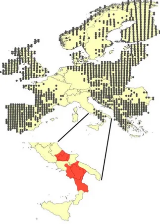
less free of otters (Ruiz-Olmo & Delibes, 1998; Kranz, 2000; Mason, 2004; Reuther & Krekemeyer, 2004) (Fig. 3). In Portugal the otter occupies more or less the whole country and in Spain the species is distributed almost regularly across the western half part of the country. In France the otter is present mainly in the western side. In Belgium, Netherland and Luxemburg there are not official data about natural populations. In Switzerland the otter has to be considered extinct. The current core of otter’s distribution in Germany is formed by the north-eastern states and in Bavaria a small population is connected with the population in Czech Republic and in Austria. In Denmark the data of the national and regional surveys give evidence that the Danish population is still expanding. In Italy the otter is present only in the southern part of the country, and this population has to be recognised as the most endangered in Western Europe because of its complete isolation. In Austria the major occurrences were found in the northern border regions to Germany and Czech Republic and in the south-eastern border regions to Slovakia and Hungary. In the countries of the Baltic coast the otter is well distributed. In the Balkan Peninsula the otter is well widespread too (Reuther & Krekemeyer, 2004) (Fig. 3).

Fig. 3 – Distribution of the otter in Europe and in Italy. The grey dots indicate the presence of the species and they are referred to 50x50km grid cell (source: EIONET).

(15)

At European level the otter is included in the List of Rare and Threatened Mammals of the Council of Europe, in Appendix II of the Berne Convention, in Appendices II and IV of the Habitat Directive of the European Union, in Appendix I of the CITES. Until the 2007 the species was classified as vulnerable in the IUCN Red List of Threatened Species (Hilton-Taylor, 2000). In the 2007 the species was downgraded to near threatened (IUCN, 2007), but its status could be raised if causal factors are not remediated (IUCN, 2007).

In Italy the species was distributed over the whole Italian country before 1950 (Cagnolaro et al., 1975), but by the end of he XX century it was confined to a small part of southern Italy (Spagnesi, Toso & De Marinis, 2002). Causes for this decline include hunting, food shortages (mainly of fish), and the destruction of riparian vegetation (Mason, 1989; Conroy & Chanin, 2000). Presently, the otter’s Italian population consists of two, apparently isolated, populations (Fig. YY) (Fusillo, Marcelli & Boitani, 2007). The otter was then included as a critically endangered in the Italian vertebrates red lists (Calvario & Sarrocco, 1997).

The need for conservation strategies for the otter

The fragmentation and the separation of the European distributions could not assure the genetic diversity necessary to ensure the long term persistence of the species (Reuther & Krekemeyer, 2004). The conservation of the otter would benefit from large scale conservation policies aiming to promote the population expansion and reconnection. Thus the identification of the large scale factors that affect wild population, the recognition of gaps of unsuitable habitats and suitable habitat for species recovering are crucial to efficiently define conservation actions (Robitaille & Laurence, 2002).

In this sense habitat suitability models are a fundamental tool for the conservation of the otter as they provide a geographic perspective for conservation strategies. For the conservation of the species it is important to understand what are the factors that affect otter distribution at large scale and to develop an habitat suitability map for the otter in Europe to predict the otter recovering in a medium to a long term.

The implications for the otter’s conservation are several; for example:

• To address conservation actions on environmental features that affect population survival;

• To identify suitable areas susceptible to be re-colonised where it would be important to limit perturbations and habitat destruction;

(16)

• To identify critical areas for dispersal, so as to improve connectivity between suitable patches;

• To discover unknown nucleus in areas of high habitat suitability (model-based sampling).

Instead, the Italian population has been slow to recover, and signs of the species’ expansion are only beginning to appear (Prigioni, Balestrieri & Remonti, 2007). The budding expansion process, the relatively small size of the otter Italian population and the presence of two disjoint populations all lend importance to the establishment of effective conservation strategies. Among conservation priorities are (i) the protection of the areas of potential otter recolonization, and (ii) a better understanding of the otter’s habitat requirements at fine scale.

1. 3 Objectives and content of the main chapters

The general aim of this PhD thesis is to assess the usefulness, effectiveness and shortcomings of habitat suitability models applied at different spatial scales to identify suitable areas susceptible to be re-colonised by the otter to establish effective conservation strategies for the species.

Given the broad scope of the issue, this will be achieved by conducting specific studies aiming to investigate important unsolved limitations and suggest new approaches.

Chapter 2 presents an approach combining a fine scale Habitat Suitability (HS) model and connectivity analysis to identify areas where the otter could potentially expand in the short-medium term within and around the south-central Italian subpopulation. The HS model was also used to identify rivers with particularly suitable habitats that could provide source populations.

Chapter 3 presents a study to test the capacity of HSMs in identifying the locations and characteristics of the areas potentially suitable for the recovery of the European otter in Italy. More generally, we expected the results to help in defining guidelines for a right use of the HSMs, especially in non-equilibrium situations, such as spreading species. We considered two species distribution datasets: the first was collected before, and the second after, a recolonization event. We assumed that the first situation was not at equilibrium, and that the second had reached a sub-equilibrium state. For HSMs, we used two common methods, one dealing with presence-only data, and the second using presence and absence data of the species. We computed and cross-validated models based on the

(17)

pre-colonization dataset and then externally validated them with the post-pre-colonization dataset. The modeling methods were deliberately chosen among the commonly used methodologies, as we wanted our results to be useful to other researchers and conservation practitioners.

Chapter 4 presents a study with the aim in determining which factors influence the otter distribution and use them to predict the potential distribution of the species in Europe, under current and future climate. The environmental variables used are related to water availability, food supply, resting site and human disturbance using six different modelling approaches. Future projections are derived by running the CCM3 climate model under a 2xCO2 increase scenario. At the European scale, the otter is mostly influenced by water availability. The current potential distribution reveals large gaps of unsuitable habitats limiting connectivity between otter populations in Europe. Climate change would have different effects on otter habitat suitability in Europe. In the Western part, the model predicts losses of suitable habitats, whereas gains are predicted in central Europe and Eastern Europe shows equal rates of losses and increases of suitable habitat. Our results are important in helping setting up conservation actions and promote otter recovery in Europe.

Chapter 5 describes the project which is in progress aiming to assessing the potential of Swiss landscapes to sustain the reintroduction of otter populations, through the development and application of a habitat suitability model, calibrated at the European scale, then projected and refined with local environmental predictors at a finer scale over Switzerland, and verified in the field.

(18)

CHAPTER 2 – HABITAT SUITABILITY AND CONNECTIVITY

FOR THE OTTER

__________________________________________________________

Otter Lutra lutra population expansion: assessing habitat suitability and

connectivity in southern Italy

Anna Loy1*, Maria Laura Carranza1, Carmen Cianfrani1, Evelina D’Alessandro1, Laura Bonesi2, Piera Di Marzio1, Michele Minotti1 and Gabriella Reggiani3

1

Università del Molise, Contrada Fonte Lappone, I-86090 Pesche, Italy; e-mail: a.loy@unimol.it

2

Università di Trieste, Via Weiss 2, I-34127 Trieste, Italy

3

Istituto di Ecologia Applicata, Via Cremona 71, I-00161 Roma, Italy

Published in Folia Zoologica 2009, issue 3

(19)

Abstract

The Eurasian otter is one of the most endangered mammals in Italy and its distribution is now restricted in two isolated portions in southern Italy. However, in recent times, this species has shown a tendency to expand its range, especially northwards. It is therefore important to identify suitable areas on the border of its expansion range where the species can establish and disperse, so that these areas can be targeted for conservation actions. To this aim, the distribution, quality and connectivity of habitats of seven river catchments located in the northern portion of the current otter range in Italy were assessed. Catchments included both rivers where the otter currently occurs and where it is likely to expand in the short-medium term. An expert-based Habitat Suitability (HS) model was developed and validated using otter presence-absence data based on standard field surveys. Fine scale riverbank land cover, extra-riparian coarse scale land cover, altitude, bank slope, and human disturbance were considered as the main factors in the HS model. These variables were available or newly created in the form of digital maps (layers) and the HS model was built by sequentially filtering these layers. Connectivity was assessed within and between river basins through landscape algorithms by taking into account variables that could influence otter dispersal. The results indicated that the seven rivers considered are heterogeneous both in terms of habitat suitability and in terms of connectivity. Among these, one river in particular (the river Volturno), where otters are currently present, showed one of the largest extensions of suitable habitats and the best connectivity both within the river and between the river and the neighbouring catchments, suggesting that this river could play a strategic role in the survival and expansion of otters in the surrounding areas.

(20)

Introduction

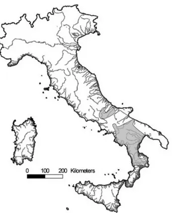
The Eurasian otter (Lutra lutra L.) is a semi-aquatic carnivore that underwent a strong decline in Europe between the 1960s and the 1980s (Mason & Macdonald 1986, Mason 1989, Macdonald & Mason 1994). Several factors have been suggested to explain this decline, including the reduction of food supply, pollutants, human persecution, and the destruction of riparian vegetation (Mason & Macdonald 1986, Macdonald & Mason 1994, Conro y & Chanin 2000, Kruuk 2006). The decrease in the concentration of harmful pollutants in the environment due to more stringent regulations (Pac yna 1999) and the enactment of legal protection have allowed otter populations to gradually recover since the 1980s in several European countries (Conro y & Chanin 2000, Roos et al. 2001, Mason & Macdonald 2004). Compared to other populations in Europe, the Italian population has recovered rather slowly, and signs of the species expanding its range have only recently started to become apparent (Prigioni et al. 2007). Despite the fact that the IUCN Red list and the European Mammal Assessment consider the Eurasian otter as near threatened (Temple & Terr y 2007, 2009; Ruiz-Olmo et al. 2008), this animal is still considered a critically endangered species in Italy (Bulgarini et al. 1998). At present, the Italian range of the otter is confined to the southern part of the Italian peninsula (Fig. 1), while originally the species was distributed all over the country (Cagnolaro et al. 1975). The residual population is relatively small (Prigioni et al. 2006a, b) and it is geographically isolated and genetically differentiated from other European populations (Randi et al. 2003). Furthermore, this population is currently separated into two isolated subpopulations (Fig. 1): the largest one located in southern Italy and the smallest one, only recently discovered, located in south-central Italy (Lo y et al. 2004, Fusillo et al. 2004, 2007, Prigioni et al. 2007).

(21)

Fig. 1 - Distribution range of the otter Lutra lutra in Italy.

The subpopulation of south-central Italy is currently expanding northward (De Castro & Lo y 2007) while there is no indication that otters are currently colonising the gap that separates the two subpopulations. Given the small size and the current expansion trend of the south-central subpopulation, it is important to identify rivers that can potentially host otters in the area and also to identify the rivers and land areas through which the species could disperse to better target conservation actions aimed at promoting the recovery of the species.

In this study, an approach combining a fine scale Habitat Suitability (HS) model and connectivity analysis was adopted to identify areas where the otter could potentially expand in the short-medium term within and around the south-central subpopulation. The HS model was also used to identify rivers with particularly suitable habitats that could provide source populations. HS models for otters have been produced on different geographic scales (Ottino et al. 1995, Prigioni 1995, Prenda & Granado- Lorencio 1996, Antonucci 2000, Reggiani et al. 2001, Barbosa et al. 2001, Boitani et al. 2002) with a resolution which is usually greater than 1 km. However, fine scale approaches are still lacking. The fine scale approach is particularly critical for otters, as some important habitat requirements such as riparian vegetation cover may not be related to the available coarse scale environmental GIS variables usually used to build HS models.

(22)

Study Area

The study area comprised seven river catchments of south-central Italy (Sangro, Biferno, Trigno, Fortore, Saccione, Sinarca, and the upper part of the River Volturno) located mostly in the Molise region (Fig. 2). These catchments comprise both rivers where otters are currently present and neighbouring rivers where otters are likely to expand in the near future.

The total length of the water courses considered in the study was 1 943 km. A standard survey run in the years 2000-2004 (Fusillo et al. 2004,Lo y et al. 2004) revealed that otter occurrence was restricted to the Biferno and upper Volturno catchments. Sporadic records of otters were also reported for the river Fortore, while otters were seemingly absent from the rivers Sangro, Trigno, Saccione, and Sinarca (Fig. 2). A more recent survey in 2006 revealed signs of otter occupation on the river Sangro, which is located in the north-western part of the study area (De Castro & Lo y 2007).

Fig. 2 - Map of the study area with the seven river catchments. Only the southern tributaries of the river Trigno and Sangro were considered, as the standard survey was limited to the river basins of the Molise region (see text). The map also shows the UTM grid cells of 10x10 km used to validate the HS model. Shadowed cells indicate otter presence. The white circles report negative otter sites, while the black ones report positive otter sites (Loy et al. 2004).

(23)

Material and Methods

Habitat Suitabilit y m odel developm ent

The HS model was expert-based, rather than inferential. There were two reasons behind this choice: 1) an inferential approach applied on the peripheral areas of an expanding species’ range may fail to discriminate between suitable and unsuitable areas because suitable areas may not yet be occupied (Jason et al. 2002, Clevenger et al. 2002, Ottaviani et al. 2004); 2) European otters have been thoroughly studied and many of the factors that influence their biology and ecology are well known (Mason & Macdonald 1986, Mason 1989, Beja 1992, Madsen & Prang 2001, Bonesi & Macdonald 2004, Kruuk 2006).

As availability of water represents a main ecological factor affecting otter occurrence (Beja 1992, Prenda et al. 2001, Bonesi & Macdonald 2004, Kruuk 2006) the model was developed on those river stretches that were likely to have water all year round. Main river courses and first and second order tributaries were selected from the national hydrographical network (1:250000 map obtained from the national environmental agency, ISPRA) and included in the model. Spatial information on the distribution of the otter’s resources and disturbance factors was derived from existing digital maps and. However, for the “bankside fine scale land cover” variable, a specific spatial data set was developed. Each variable was inserted into a G.I.S. system as a different layer and all categories within each variable were reclassified according to their suitability for otters (Appendix 1). More specifically, the following variables were considered:

Bankside fine scale land cover (1:5000). Many studies have found relationships between the number of otter signs and bank side cover (Jenkins & Burrows 1980, Macdonald & Mason 1982, 1985, 1988, Bas et al. 1984, Adrian 1985, Prauser 1985, Delibes et al. 1991). As this parameter is not detectable from the usual coarser CORINE land cover maps, data were obtained by digitising land cover categories derived from aerial photos taken in 2005 and considered at a resolution of 20 m. This variable was considered on a 300 m large buffer around the river. The categories used were those of the CORINE land cover classification scheme at the third level of detail (European Commission 1993). The procedure of assessing land cover from aerial photos at a scale of 1:5000 allowed us to gain a good representation of the riparian vegetation on and around the river banks. The role of riparian vegetation was then considered according to its use in providing breeding dens, enhancing the filtering of pollutants and promoting fish productivity (Jenkins & Burrows 1980, Green et al. 1984, Macdonald & Mason

(24)

1994, Rader 1997, Morrow & Fischenich 2000). The CORINE land cover categories were then re-classified accordingly (Appendix 1 – layer 1 in Fig. 3).

Bank slope. A slope layer was derived from the Digital Elevation Model at a resolution of 20 x 20 m. Cells within the buffer area with a slope of 70° or more were considered as evidence of rock cliffs, potentially providing good sites for resting and breeding dens (Chanin 2003), and were classified as highly suitable (Appendix 1 – layer 1 in Fig. 3).

Altitude. This variable is important because otters are rarely found above 2000 m a.s.l., probably due to the scarcity of food available at high altitudes (Ruiz-Olmo 1998, Kruuk 2006). We used the 20 m resolution Digital Elevation Model to classify the area into four altitudinal ranges of decreasing suitability (Appendix 1), producing a new layer (layer 2 in Fig. 3).

Human density. This variable can potentially affect the presence of otters negatively (Barbosa et al. 2001, Chanin 2003) and was derived by considering the density of people in each municipality within a buffer of 1 km surrounding the river (Appendix 1 – layer 4 in Fig. 3).

Coarse scale extra-riparian CORINE land cover (1:100 000 map, year 2000). Extra-riparian disturbance was considered within a buffer of 1 km surrounding the river. The presence of land types such as urban settlements and intensive agricultural areas were considered to have a potentially negative affect the presence of otters (Barbosa et al. 2001, Boitani et al. 2002). Land cover maps were rasterized to 1 x 1 km grid cells and reclassified according to presence/absence of a negative effect (Appendix 1 – layer 4 in Fig. 3).

All GIS layers described above and saved in a raster format at a resolution of 20 x 20 m were then integrated following the scheme presented in Fig. 3 to produce the final layer of habitat suitability for the otter. First of all, the bank slope layer was overlapped to the bank side fine scale land cover layer. Cells with bank slopes which were steeper than 70° were given a high suitability value (three). When a cell had a bank-slope value of three, this figure was retained irrespective of the value of the bank side fine scale land cover, to take into account the fact that when rock cliffs are present the surrounding land cover matrix may have little influence on otter presence. The resulting layer was characterized by 20 x 20 cells with HS integer values ranging between zero and three (layer 1). This layer was then combined with the altitude layer (layer 2) to produce four synthetic suitability classes ranked between zero (less suitable) and three (most suitable) through a logical overlay operation. This operation assigned a suitability class value to each 20 m cell by

(25)

choosing the lowest value between those of the two input layers (1 and 2). The new layer (layer 3) so created was also made of integer numbers ranging between zero and three (Fig. 3). Human disturbance was then taken into consideration by subtracting values of 0.25 or 0.50 from this new layer if, respectively, one or both disturbance factors (human density and unfavourable land cover) were present (layer 4). If no disturbance was present, the layer retained its original value. The maximum number of final suitability classes resulting from this procedure was ten, ranging in values from zero (least suitable) to three (most suitable) (Fig. 3) and these values were assigned to each 20 x 20 m cell within a buffer of 300 m surrounding the river.

Habitat Suitabilit y Model vali dati on

Validation of the HS map resulting from the application of the model described above was performed using available data on the presence and absence of otters in the area derived from a standard otter survey (Lo y et al. 2004). Otter presence/absence was reported in UTM grid cells of 10 x 10 km, considering only the river basins of current otter occupancy, for a total 42 UTM grid cells (Fig. 2). The river Trigno was excluded from the validation analyses as it was the furthest away from areas with otter presence. Hence, it is likely that the absence of otters along this river is due to the fact the species has yet to arrive there rather than to the characteristics of the river. The UTM grid cells were classified as positive (17 out of 42) if they contained at least one positive site where otter signs (spraints or footprints) had been recorded. Both presence and absence data were considered for the validation of the model. It must be stressed that absence data obtained for this species using the standard surveys are considered to be more reliable than for other species for which absence is more likely to mean non detection (Reuther et al. 2000). The percentage of the 300m buffer around the river covered by each of the ten suitability classes was computed within each UTM grid cell of 10 x 10 km. The percentage area covered by each HS class was then compared between 10 x 10 km UTM grid cells which were positive or negative for otters through a non parametric Mann–Whitney U-test.

Accuracy of the model was then tested through a sensitivity analysis for HS classes showing significant differences either for presence or absence of otter signs. Sensitivity analysis was performed by applying the ROC (Receiver Operating Characteristics) technique (Fielding & Bell 1977, Swets 1998, Manel et al. 1999, Greiner et al. 2000, Osborne et al. 2001). The suitability classes that successfully passed the test were used to define a threshold between two large categories of suitable and non suitable habitats.

(26)

Fig. 3 - Flow chart of the procedure used to create the 10 HS suitability classes. The first number in each cell of the square matrix in the middle represents layer 1, while the second number represents layer 2. The dotted square on the right represents the process of subtracting human disturbance (human density and land cover derived from the CORINE 1:100 000) from layer 3.

Connecti vit y an alysi s

Otter habitats tend to develop along linear features of the landscape, namely the hydrographical systems (Philcox et al. 1999, Kruuk 2006). Analyses examining the connectivity of the landscape along linear features such as rivers are relatively new (Bennett 1999, Wiens 2002, Schick & Lindle y 2007) and pose some specific problems in that both longitudinal and lateral connectivity must be evaluated (van Langevelde et al. 1998). Longitudinal connectivity refers to otters moving within one river system, while lateral connectivity refers to dispersal movements toward neighbouring rivers, which contribute to range expansion and the maintenance of gene flow among populations living in different river basins. As river catchments can be considered as closed systems, the longitudinal connectivity can be simply evaluated through the distribution of suitable habitat patches, while the lateral connectivity must also consider the resistance (permeability) of the land matrix to dispersal by otters between catchments (Schumaker 1996, Tischendorf 2001).

Longitudinal connectivity along rivers was analysed by summarising two classical spatial pattern statistics of suitable habitat distribution (Mac Garigal & Marks 1995, McGarigal et al. 2002). More specifically, the extension and fragmentation of suitable

(27)

patches, as identified by the HS model, within the 300 m buffer along rivers were evaluated through their number patches (NUMPs) and mean patch size (MPSs). These data were evaluated considering the mean distance covered by an otter during its daily movements in Italian river catchments, which was respectively 10 km for males and 6 km for females (Di Marzio 2004).

Lateral connectivity was assessed by evaluating the resistance of the land matrix between neighbouring catchments to otter movements, i.e. dispersal. The following layers of the land matrix were considered to be relevant in evaluating resistance to otter dispersal: slope, land cover, altitude, human density and road networks (Philcox et al. 1999, Janssens et al. 2006). The analysis was performed within the region Molise area, for which all GIS layers were available. Source of data for slope, altitude and land cover were the same as those specified for the HS model; road networks were derived from a 1:250 000 digital map of the National Environmental Agency (ISPRA). Specifically, slopes were considered to be impermeable when greater than 45° (Cortés et al. 1998, Saavedra & Sargatal 1998, Saavedra 2002, Janssens et al. 2006); altitude, CORINE land cover map at scale 1:100 000, and roads were reclassified for permeability as listed in Appendix 1. All the reclassified layers were then rasterized at a resolution of 20 x 20 m. The logical overlay of the considered layers allowed the identification of areas which were permeable to otter dispersal between catchments. A group of contiguous 20-meter permeable cells formed a permeable patch. The efficacy of each permeable patch was analysed considering its extension and the number of river tributaries connected within it. To this aim, we considered the whole hydrographical network at a resolution of 1:250 000 (source ISPRA), rather than only the main course and main tributaries as in the HS model.

Results

HS m odel results an d validation

Of all the ten HS classes resulting from the HS model, only three held sufficient data for the validation analysis (Fig. 4). The Mann–Whitney U-tests revealed significant differences between positive and negative UTM cells for the HS classes with values of 0.75, 1 and 3 (p < 0.05 for all pairwise comparisons). HS classes 1 and 3 were found to be significantly associated with the presence of otters, while the 0.75 class was significantly associated with their absence. No significant difference was reported for the other HS categories, which is probably due to their small sample size.

(28)

Fig. 4 - Mean and SD of suitable (filled bars) and unsuitable (empty bars) areas computed for HS classes within each UTM cell shown in Fig. 2. Asterisks indicate HS classes showing significant differences between presence-absenceUTM cells (Mann-Withney U, p < 0.05).

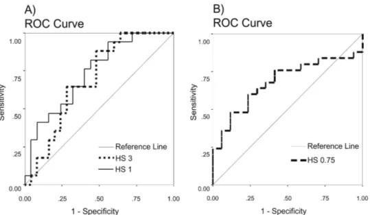
The three significant HS classes with values of 0.75, 1 and 3 were subjected to a sensitivity analysis using ROC curves. For HS class 1 and 3, the Area Under the ROC curve (AUC) had, respectively, the values of 0.74 and 0.69, suggesting that they were able to discriminate the presence of otters relatively well (Fig. 5A). The ROC plot to test for the sensitivity of the HS class 0.75 was used to evaluate its ability to predict otter absence, rather than presence (Fig. 5B). Also in this case, an AUC value of 0.68 suggested a good probability of a correct prediction.

Fig. 5. A – ROC plot for the HS values 1 and 3, testing the accuracy to predict the presence of otters. B – ROC plot for the HS value 0.75, testing the accuracy to predict the absence of otters.

(29)

Based on the above results, we considered 0.75 as a threshold value and a new HS map was hence produced by reclassifying all 20 x 20 m cells as non-suitable or suitable, according to whether they were, respectively, above or below this HS value (Fig. 6).

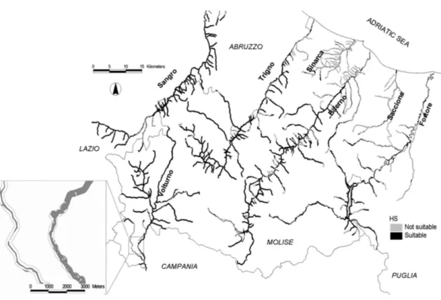
The river Biferno, followed by the river Sangro, Trigno and Volturno were identified by the HS model as the ones with the highest suitability for otters (Figs. 6 and 7). Suitable areas were concentrated in the upper and medium course of the rivers, while the lower plains were generally unsuitable for otters. A small concentration of suitable areas was also found in the upper river Fortore, where scattered otter signs were found, whilst its lower course and the whole course of the rivers Sinarca and Saccione were classified as unsuitable for otters.

Fig. 6. Map showing the distribution of suitable (HS ≥1) and unsuitable (HS < 1) habitat patches for the seven river catchments of the study area.

(30)

Fig. 7. A – Comparison of the total buffer extension and total surface of suitable habitat for each river basin. B – Mean size (MPS) and number (NUMP) of suitable patches for the same river basins.

(31)

Fig. 8 - Results of the lateral connectivity analysis for the river catchments within the region Molise. Patches are shaded according to the degree of permeability to otter moving across the watersheds.

Connecti vit y an alysi s

The analysis of the distribution and extension of suitable patches along rivers (longitudinal connectivity) indicated that the river Volturno had the best connectivity having the largest extension of suitable patches and the most connected patches (Fig. 7). The rivers Biferno, Trigno and Sangro had also, overall, a relatively large extension of suitable patches, but their distribution was quite different from the suitable patches on the Volturno. Indeed, on these three rivers suitable patches tended to be numerous but highly fragmented.

The map in Fig. 8 reports the results for lateral connectivity and highlights a concentration of areas of the land matrix that are likely to be permeable to otter movements located between the upper river Volturno and the river Sangro, Trigno and Biferno, whilst permeable areas between the other catchments are less extended and more fragmented. The high permeability around the upper reaches of the Volturno probably allowed the recent

(32)

otter expansion to the Sangro river basin (De Castro & Lo y 2007), and will likely lead to the recolonization of the river Trigno in the short term.

Discussion

The fine scale HS model adopted in this study was well able to discriminate between areas with and without signs of otters for the subpopulation living in the northern portion of the Italian otter range, suggesting that riparian vegetation cover (fine scale land cover), bank slope, altitude, and human disturbance (human density and extra-riparian land use) can be useful factors for assessing the probability of otter presence or absence in an area. Riparian vegetation may be important for otters for several different reasons: it provides resting and breeding dens, provides cover during movements, enhances filtering of pollutants, and promotes fish productivity (Jenkins & Burrows 1980, Green et al. 1984, Macdonald & Mason 1994, Rader 1997, Morrow & Fischenich 2000). It is possible that in Italy vegetation cover may play a particularly important role in protecting the animals from human and human-related disturbance. Indeed, human disturbance is likely to be particularly important in constraining the distribution of otters in southern and central Italy because otters are still illegally killed (Laura Bonesi, unpublished data), rivers are often surrounded by areas with a relatively high human population density, and feral dogs, that are known to be a threat to otters (Marjana Hönigsfeld, pers.obs.), are often present. While these threats are still also common in other Mediterranean countries (e.g. Robitaille & Laurance 2002), all or most of them are often absent from areas or countries, like for example the UK, where otters are known to live along rivers with scarce or absent riparian vegetation and which even frequent urban environments (Crawford 2003). Similarly to riparian vegetation, steep rocky banks, which are taken into account in the model with the variable “bank slope”, may be important as they provide protection from disturbance because they are not easily accessible overland by both humans and dogs. Ruiz-Olmo et al. (2005) in their study of female otters with cubs in north-east Spain also found that otters, in particular older cubs, tended to be concentrated around areas which were well protected by steep rocky cliffs. Finally, altitude may play a role as usually the upper reaches of the streams that are found at higher altitudes tend to host a less diverse community of fish and fish biomass is less abundant (Ruiz-Olmo 1998). Compared to other HS models developed for otters (Ottino et al. 1995, Prigioni 1995, Prenda & Granado-Lorencio 1996, Antonucci 2000, Barbosa et al. 2001, Reggiani et al. 2001, Boitani et al. 2002), our model was based on a much finer scale as it considered habitat variables at a resolution of 20 x 20 m. We think that working at this fine scale resolution may provide a management tool that allows an accurate identification of specific sites along rivers which could benefit from special

(33)

protection or from specific improvements that may favour the otter. The model of matrix permeability was able to identify overland areas where corridors which would favour otter dispersal are more likely to occur within and between catchments, thus offering a tool for the management of the extra-riparian landscape for otter conservation. The identification of suitable habitat patches for otters within rivers, along with the assessment of the permeability of the land matrix to dispersal and the presence/absence data, provide a general framework to interpret the otter’s movements within and between river basins and to make an assessment of each catchment in terms of its ability to host source or sink populations. Among all the seven catchment considered, one river in particular (the river Volturno), where otters are currently present, showed one of the largest extensions of suitable habitats and the best connectivity both within the river and between the river and the neighbouring catchments, suggesting that this river could play a strategic role in the survival and expansion of otters in the surrounding areas, and in the joining of the two isolated portions of otter range.

In fact, otters at present occur in two portions of this river basin, the upper Volturno in the south central range, and one of its tributary in the southern range. Thus the colonization of the medium course of this river will likely allow the joining of the two ranges in the short-medium term.

In spite of the ability of the HS model to predict relatively well presence and absence of otters at a 10 x 10 km resolution, there are, however, a number of limitations to our model. First of all, the model is based on the distribution of spraints and not on the distribution of the actual animals, but there are two factors that may mitigate this limitation. First, in otters, spraints are likely to be used to signal the use of resources such as food and dens, rather than reproductive status or aggressive encounters, at least when they live in groups such as on the Shetland coast (Kruuk 1992). In freshwater areas, otters live at lower densities than in coastal areas and tend to be more solitary, although their home ranges may still overlap, especially between males and females (Kruuk 2006). If in freshwater areas, spraints are also used to signal the use of resources, then the distribution of spraints may be considered as an acceptable surrogate for the distribution of otters in HS models which consider variables that are directly linked to the use of resources or disturbance, such as ours. Second, to validate the model, we considered a spatial scale of 10 x 10 km, which is in the order of magnitude of an otter’s home range, i.e. 10-20 km (Antonucci 2000). Probably due to the fact that we considered relatively large validation cells of 10 x 10 km and a relatively large study area with enough variability, the use of spraints as surrogates for otter distribution was not particularly limiting because the

(34)

suitability of a relatively large area around the 600 m sites with signs of otters was considered.

Another limitation to our model was that we were unable to take into account one of the most important resources for otters: fish availability (Kruuk et al. 1993, Jeņdrz ejewska et al. 2001, Lanszki & Sallai 2006). Reliable data on fish community composition and biomass are difficult to obtain over large areas. Moreover, translating these data into actual availability of fish for otters is a further obstacle. However, for five of the seven catchments considered in this study (Sangro, Biferno, Volturno, Fortore and Trigno) data on fish biomass collected at 54 sampling stations (Regione Molise 2004) were available (Loy et al. 2008). On average, a fish biomass of 13.08 gr/m2 was registered across these five catchments (range: 0.01-98.60 gr/m2, SD = 4.08, n = 54 sampling stations). Kruuk et al. (1993) demonstrated that otters could successfully exploit oligotrophic streams populated mainly by salmonids with fish biomass between 9 and 14 g/m2, while Ruiz-Olmo (1998) noted that otters were present at sites with biomass values of 10–20 g/m2. Taking all studies that relate otter distribution with fish biomass into consideration, Chanin (2003) proposed that, as a rule of thumb, otter populations can survive and breed where fish biomass exceeds 10 g/m2. Therefore, the values that are reported for five of the seven catchments considered in this study would seem to be sufficient, on average, to support a population of otters. It was, however, not possible to incorporate these values into the model because of the relative scarcity of sampling stations for fish biomass relative to the whole study area.

The application of the HS model to the six catchments (the Trigno was excluded) resulted in only three of the ten HS classes being significantly related to the presence-absence of the species. This is probably due mainly to the fact that only these three classes were significantly represented in our sample, all the other classes being found at a relatively low frequency.

The planned extension of this approach to study the southern Italian subpopulation, together with the development of an inferential approach and the implementation of more sophisticated algorithms for longitudinal and lateral connectivity analysis, currently in progress, will probably help to improve the prediction ability of the HS and connectivity models and to offer better insights into the areas of potential range expansion of otters in Italy and into the likelihood that the two subpopulations will become connected in the future.

(35)