Article
The Role of Orthogonal Polynomials in Tailoring
Spherical Distributions to Kurtosis Requirements
Luca Bagnato, Mario Faliva and Maria Grazia Zoia *
Dipartimento di Discipline matematiche, Finanza matematica ed Econometria, Università Cattolica del Sacro Cuore, Largo Gemelli 1, Milano 20123, Italy; [email protected] (L.B.); [email protected] (M.F.) * Correspondence: [email protected]; Tel.: +39-02-7234-2948
Academic Editor: Charles F. Dunkl
Received: 14 July 2016; Accepted: 30 July 2016; Published: 5 August 2016
Abstract: This paper carries out an investigation of the orthogonal-polynomial approach to reshaping
symmetric distributions to fit in with data requirements so as to cover the multivariate case. With this objective in mind, reference is made to the class of spherical distributions, given that they provide a natural multivariate generalization of univariate even densities. After showing how to tailor a spherical distribution via orthogonal polynomials to better comply with kurtosis requirements, we provide operational conditions for the positiveness of the resulting multivariate Gram–Charlier-like expansion, together with its kurtosis range. Finally, the approach proposed here is applied to some selected spherical distributions.
Keywords: orthogonal polynomials; spherical distributions; Gram–Charlier-like expansions; kurtosis
1. Introduction
It is well known that a set of orthogonal polynomials can be associated to a density function with existing moments of all order. This clears the way for the tailoring of the shape of a given distribution from “inside” through a polynomial shape-adapter, built on the orthogonal polynomials engendered by the same distribution (e.g., [1–4]).
So far, this method—which can be viewed as an inheritance of the Gram–Charlier expansion—has proved effective when applied to distributions to account for possibly severe kurtosis and skewness (e.g., [5,6]). In this paper, we gain further insight into the matter and work out a similar orthogonal-polynomial-based approach to increasing the values of the moments—in particular, the fourth—within a multivariate spherical framework. Spherical distributions—a particular class of elliptical distributions [7,8] whose contours of equal density have spherical shapes—prove effective in several applications, such as portfolio theory and the capital asset market (e.g., [9,10]). However, it sometimes happens that the kurtosis of such a distribution is lower than required, thus imposing the need for a reshaping to duly fit in with empirical evidence.
After running through the procedure to derive a spherical distribution via a density generator, the Gram–Charlier-like expansion is duly specified, and the involved orthogonal polynomial derived in terms of the moments of the so-called modular variable (see AppendixA).
The paper proceeds as follows. Section2sets the groundwork by providing a determinantal representation of orthogonal polynomials in terms of closed-form expressions of the moments of the weight function, paving the way for the notion of Gram–Charlier-like expansion. Section3
addresses the issue of the density reshaping problem via orthogonal polynomials in a multidimensional framework on a spherical distribution argument. Section4, focusing on kurtosis behavior, deals with the orthogonal-polynomial approach to density reshaping by investigating a few selected spherical laws—namely, the Gaussian, the logistic, and the hyperbolic secant ones, their Gram–Charlier-like
expansions, and the related moments. Section5 presents some concluding remarks. Finally an appendix, devoted to spherical laws, completes the paper.
2. Orthogonal Polynomials and Related Gram–Charlier-Like Expansions
Recently, Zoia et al. have shown how to modify the moments of a univariate distribution f(.) by making use of Gram–Charlier-like expansions based on orthogonal polynomials associated to f(.) [3,6]. In this regard, the monic orthogonal polynomial of degree h, with density f(x) as weight function, is defined in terms of the moments of f(x) as follows [11]:
phpxq “ detM1 hdet « Mh hh x1h xh ff “`ah`1,h`1˘´1 h ÿ k“0 ak`1,h`1xk (1) where Mh ph,hq“ » — — — — – m0 m1 ¨ ¨ ¨ mh´1 m1 m2 ¨ ¨ ¨ mh ... ... ... ... mh´1 mh ¨ ¨ ¨ m2h´2 fi ffi ffi ffi ffi fl (2) x1h p1,hq“ ” 1, x, ...xh´1ı (3) h1h p1,hq“ rmh, mh`1, ...m2h´1s (4) mi “ 8 ª ´8 xif pxqdx, j “ 0, 1, 2 (5)
and aij denotes the (i,j) entry of the adjoint of the Hankel moment matrix Mh`1, noting that
ah`1,h`1 “ detMh. In the following, we will assume to operate with even density functions of
standardized variables. Odd moments vanish accordingly, and orthogonal polynomials phpxq are even
functions if h is even, and odd otherwise.
As already remarked, the moments of a density function f (.) can be modified to some extent by moving to a properly chosen Gram–Charlier-like expansion 'p.q built on its own orthogonal polynomials. In particular, consider an expansion specified as follows
'px, q “ qjpx, q f pxq (6)
where
qjpx, q “ 1 `e
jpjpxq (7)
Here j is even, > 0 subject to 'px, q being positive, and pjpxq and ejare given by
pjpxq “`aj`1,j`1˘´1 j{2 ÿ l“0 a2l`1,j`1x2l (8) ej“ 8 ª ´8 p2jpxq f pxqdx “ 8 ª ´8 xjpjpxq f pxqdx “`aj`1,j`1˘´1 j{2 ÿ l“0 a2l`1,j`1mj`2l (9)
respectively. From the properties of the orthogonal polynomials, it follows that the moments µiup to the j-th order of 'px, q are the same as the moments miof the parent density f (.). That is,
More generally, we prove the following
Theorem 1. The moment of order 2h • j of 'px, q is an algebraic function of the even moments of f(x) of order up to 2h + j, which varies linearly with b, that is
µ2h“ m2h` j{2 ∞ l“0a2l`1,j`1m2h`2l j{2 ∞ l“0a2l`1,j`1mj`2l (11)
Proof. The proof follows in a straightforward manner from the representation (8) ofpjpxq; bearing in
mind (9).
In light of Theorem 1, factor (7) reshapes the density f(x) by modifying its j-th moment to the extent of , and in so doing, it operates as a polynomial shape adapter.
If we were interested in modifying more than one moment of the parent density f(x), a similar argument could be advanced by making use of a properly designed polynomial shape adapter depending upon the orthogonal polynomials corresponding to the moments to be adjusted. Further, this polynomial approach to density reshaping can be given a multivariate formulation from a spherical distribution standpoint, as we will show here below.
3. Multivariate Extensions via Spherical Distributions
In what follows, the issue of density reshaping based on orthogonal polynomials will be extended to n-dimensional spherical distributions (see AppendixA). As a premise, in order to single out the polynomial shape adapter for reshaping a spherical density, let us recall that the density function gnpxq of a spherical variable can be conveniently expressed in terms of the density fRp.q of its modular
variable R (see AppendixA) as follows
gnpxq “ k fRpx1xq1{2 (12)
where
k “ Gpn{2q 2p⇡qn{2px
1xq1´n (13)
with Gp.q denoting the Euler Gamma function.
As a by-product, the moments of R determine the moments of the spherical variable (see [8,12]). It follows that a change in an even moment of the modular variable will affect the even moments of the parent spherical one.
Now, let us reshape fRprq by means of a j-th degree polynomial
qn,jpr, q “ ˜ 1 `e jpjprq ¸ (14) where pjprq is defined as in (8), and let
fRrprq “ qn,jpr, qk fRprq (15)
be the resulting density. According to (12), the density of the reshaped spherical vector is given by 'npx, q “ kqn,jpx, q fRpx1xq1{2“ qn,jpx, qgnpxq (16)
The above formula provides the Gram–Charlier-like expansion of the spherical density gnpxq
obtained via the polynomial adapter (14) in the argument px1 xq1{2, where x1“ rx1, x2, ...xns.
In the following, we will focus on a polynomial correction hinging on the 4-th degree orthogonal polynomial, which is intended to reshape the parent distribution gnpxq so as to meet kurtosis
requirements to the required extent. By setting j = 4, the polynomial adapter (14) becomes qn,4px, q “ ˆ 1 `e 4rpx 1 xq2 ´ e2px1xq ` e0s ˙ (17) and gives rise to a Gram–Charlier-like expansion tailored to embody certain facts, such as fat tails and accentuated peakedness peculiar to financial data, whose manifestation is a possibly severe kurtosis.
Following [8], the kurtosis K of an n-dimensional spherical variable is defined as follows K “ n2 EpR4q
rEpR2qs2 (18)
and can be read as n2times the kurtosis of a symmetric zero mean univariate variable Z such that
Z=|R| with12f pRq as density.
According to (18), an increase in kurtosis of a spherical variable can be obtained by pushing up the fourth moment of its modular variable. This can be done by reshaping R via the fourth degree polynomial (17). The parameters e2j, j = 0,1,2, defined in accordance with (9), can be computed
as follows: e4“ pm8´ e2m6` e0m4q, e2“ m6´ m4m2 m4´ m22 , e0“ m6m2´ m 2 4 m4´ m22 (19) in terms of the moments mjof the modular variable R.
In this regard, we have the following:
Theorem 2.The moments of order j, denoted with mj, of the modular variable R are given by
mj“
`n
2˘j{2cn
pj{2cn`j (20)
where paqb“ Gpa`bqGpaq is the Pochhammer symbol, cgis defined as follows
c “ Gp {2q
p⇡q /2 8r
0 y
/2-1gpyqdy
(21)
And gp.q denotes the density generator of the parent spherical variable (see AppendixA).
Proof. According to [8], the j-th moment of the modular variable R is given by
mj“ 8 r 0 y pn`jq{2´1gpyqdy 8 r 0 y n{2´1gpyqdy (22)
which, taking into account (21), can be written as in (20).
Assuming this, the Gram–Charlier-like expansion of a spherical distribution gnpxq designed to fit
in with the empirical evidence of possibly severe kurtosis is thus given by
where qn,4px, q is as in (17) with coefficients given by (19), and > 0 subject to 'npx, q being positive.
In this connection, we have the following
Theorem 3.The Gram–Charlier-like expansion (23) is positive if satisfies the following inequalities 0 § † ` 4e4
e2
2´ 4e0˘ “
˚ (24)
Proof. The function 'npx, q is positive provided the polynomial p4p.q is also. Now, some computation
proves that
p4pxq • p4e0´ e 2 2q
4 (25)
where the right-hand side of the above formula is a negative quantity. It follows that ˆ 1 `e 4p4pxq ˙ ° 0 (26) as long as satisfies (24).
4. Polynomial Expansions of Some Spherical Distributions
In this section, the fourth order polynomial shape adapters for selected n-dimensional spherical variables are devised. The distributions considered are the Gaussian, the logistic, and the hyperbolic secant. These distributions, once polynomially adjusted, prove to be effective in handling series with different degrees of excess kurtosis. Before stating the theorems we are primarily interested in, we need the following
Lemma 1. The moments mj of the modular variable R, needed to determine the parameters e2j , j = 0,1,2,
of the shape adapter qn,4px, q , take the closed forms here below, for the spherical Gaussian, logistic, and
hyperbolic secant laws, respectively. (i) Spherical Gaussian (G),
mGj “ 2j{2´ n2
¯
j{2 (27)
(ii) Spherical logistic (L), mLj “
#
upn, jqpln2q´1Gpj ` 2qzpj ` 1q, i f n “ 2
upn, jqp1 ´ 22´nq´1pnqjz´1pn ´ 1qzpn ` j ´ 1q, otherwise (28) (iii) Spherical hyperbolic secant (HS),
mHS j “2fjpn ` jqfpnq⇡jpnqj. (29) Here upn, jq “ˆ ?3 p ˙j p1 ´ 22´n´jq (30) and fpnq “ txpn, 1{4q ´ xpn, 3{4qu (31)
Proof. Formulas (27)–(29) ensue from (20) upon noting thatc , defined as in (21), becomes
cG “ p2⇡q´ {2 (32)
for the spherical Gaussian in light of (A8). This same parameter c becomes
cL“ $ & % ⇡ 24ln2 i f “ 2 8p?3q p1 ´ 22´ q⇡´ {2zp ´ 1q`2˘p 2q otherwise (33) for the spherical logistic in light of (A9).
Finally, c becomes
c “ `2 ´2⇡ {2
2˘2 fp q
(34) for the hyperbolic secant in light of (A10).
Theorem 4. The Gram–Charlier-like expansions of the spherical Gaussian, logistic, and hyperbolic secant densities are, respectively, given by
'Gnpx, q “ qn,4G px, qp2⇡q´n{2e´px1xq{2 (35) 'Lnpx, q “ $ ’ & ’ % qn“2,4L px, q ⇡ 24ln2sech2 ´ ⇡ 2?3px1 xq 1{2¯ i f n “ 2 qL n,4px, q ⇡ n{2 8p?3qnp1´22´nqzpn´1qpn 2qp n2 qsech 2´ ⇡ 2?3px1xq 1{2¯ otherwise (36) 'nHSpx, q “ qn,4HSpx, q`2nn´2⇡n{2 2 ˘ n 2 fpnq sech´ ⇡2 px1 xq1{2¯ (37) where for each distribution, the coefficients of the polynomial qn,4px, bq are evaluated according to (19) from the
moments of the corresponding modular variable as per (27)–(29). The expansions (35)–(37) are positive subject to (24).
Proof. The proofs of (35)–(37) follow from (23) by making use of Lemma 1 for the evaluation of the
coefficients of the polynomial qn,4px, q and Theorem A2 in AppendixAfor the spherical representation
of the distributions in hand.
The analysis of the kurtosis level attainable by a spherical Gram–Charlier-like expansion as compared with that of the parent spherical law is of major interest, not only from an analytical standpoint but also for operational purposes. Based on this, we can state the following
Theorem 5. The increase in kurtosis iKp q, achievable when moving from a spherical density to its
Gram–Charlier-like expansion, is
iKp q “ 4⇡2ˆ cn`2c n
˙2
(38) where b is a parameter subject to (24).
Proof. Formula (38) can be easily established by noting that (bearing in mind Theorem 1) the effect of
the polynomial shape adapter is to increase the fourth moment of R by a quantity equal to b. Hence, it follows from (18) that the increase in kurtosis of the Gram–Charlier-like expansion is equal to
iKp q “ n2
which, by making use of (20), is the same as (38).
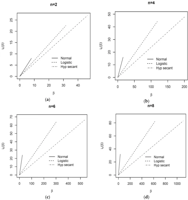
Looking at (38), we can see that the increase in kurtosis depends on both and n via the coefficient cn. The following charts shed some light on the behavior of kurtosis on either and n,
or both, as they vary.
Figure 1 shows iKp q as a function of for the three aforementioned Gram–Charlier-like
expansions for different values of the dimension n. For each expansion, iKp q attains its maximum
value in correspondence with the upper bound ˚ of as per formula (24). Looking at the graphs in Figure1, we see that, as for the univariate case, the higher the fourth moment of the modular variable R, the higher the upper bound of and of iKp q in turn. Figure2shows iKp q for the three
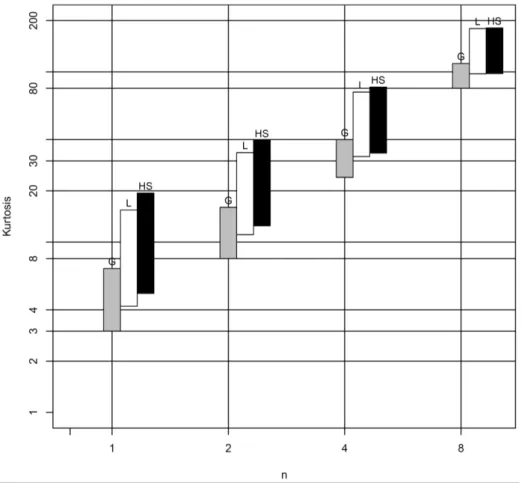
Gram–Charlier-like expansions, as a function of n in correspondence to the two values of , the upper bound ˚ and half of the same (Figure2a,b). Figure3shows the kurtosis ranges of the Gram–Charlier expansions for increasing values of the dimension n.
(a) (b)
(c) (d)
Figure 1. Kurtosis uplift,iKp q, for spherical Gram–Charlier-like Gaussian, logistic, and hyperbolic secant expansions as a function of , 0 § § ˚, and for different values of n: (a) n = 2; (b) n = 4; (c) n = 6; (d) n = 8.
(a) (b)
Figure 2. Kurtosis upliftiKp q, as a function of n in correspondence with (a) “ ˚, and (b) “12 ˚.
Figure 3. Kurtosis ranges of Gram–Charlier-like expansions of Gaussian (G); logistic (L); and hyperbolic secant (HS) laws for different dimensions n = 1, 2, 4, 8 (log scales).
5. Concluding Remarks
In this paper, the orthogonal-polynomial approach to density reshaping is developed in a multivariate framework on a spherical distribution argument. This paper extends recent insights (see [3,5,6]) on the issue of tailoring distributions in order to account for over-kurtosis. Starting from a given spherical distribution, the orthogonal polynomials of its related modular variable are
provided and used to design the intended distribution shape adapter. This allows us to specify a Gram–Charlier-like expansion whose moments can be tailored to match empirical evidence requirements. The paper basically focuses on the fourth moment, and the approach provides expansions of the spherical Gaussian, logistic, and hyperbolic secant laws, which are well-equipped to handle possible severe kurtosis occurring at a multivariate level.
Appendix A
Spherical distributions and the corresponding random vectors are also called “radial” [13] or “isotropic” [14], because they correspond to the class of rotationally-symmetric distributions. In this
connection, we have the following
Definition A1.Let x be an n-dimensional random vector. The vector x is said to be “spherically distributed” if and only if
x “ Tx (A1)
for every n-dimensional orthonormal matrix T. Any spherical random vector can be expressed, accordingly, through a stochastic representation of the form
x “ RUpnq (A2)
where R = px1xq1{2is a non-negative random variable, called modular variable, independent of Upnqwhich is uniformly distributed on the unit hypersphere with n ´ 1 topological dimensions.
A nice property of the spherical distributions is that their densities may be expressed via the density function of the modular variable, provided this is absolutely continuous.
In this regard, we state the following
Theorem A1.An n-dimensional random vector x of a standardized variable has a spherical density of the form
gnpxq “ k fRpx1xq1{2 (A3) where k is defined as in (13), fRprq “ 2r n´1 8 r 0 y n{2´1gpyqdygpr 2q (A4)
is the density of its modular variable R, and g(.) is a non-negative Lebesgue measurable function defined on the positive axis called density generator.
Proof. For the proof, see [15].
In particular, as for the spherical distributions associated with the Gaussian, logistic, and hyperbolic secant laws, we state the following
Theorem A2.The n-dimensional spherical Gaussian (G), logistic (L), and hyperbolic secant (HS) distributions denoted by gG
npxq, gnLpxq, and gnHSpxq, respectively, have the following closed forms,
gGnpxq “ p2⇡q´n{2e´px1xq{2 (A5) gLnpxq “ $ ’ & ’ % ⇡ 24ln2sech2 ´ ⇡ 2?3px1xq 1{2¯ i f n “ 2 ⇡n{2 8p?3qnp1´22´nqzpn´1qpn 2qp n2 qsech 2´ ⇡ 2?3px1xq 1{2¯ otherwise (A6)
gnHSpxq “ 2 n´2⇡n{2 `n 2˘n 2 fpnq sech´ ⇡ 2 px1xq 1{2¯ (A7)
where the symbols have the same meaning as in Lemma 1.
Proof. The density function of the modular variable underlying the spherical normal density can be
easily obtained by taking as density generator gpxq “ e´12x, and by setting s “ 12 and t “ n2 in the
Mellin transform (see [16])
8
ª
0
x⌧´1e´sxdx “ 2´⌧G p⌧q (A8)
Then, a simple computation, bearing in mind (A3) and (13), yields (A5).
The density function of the modular variable underlying the spherical logistic density can be easily obtained by taking gpxq “ sech2p ⇡
2?3x1{2q as density generator, and by setting a “ 2?⇡3 and
⌧“n2in the Mellin transform (see [17]),
8 ª 0 x⌧´1 ch2paxqdx “ # 1 a2ln2, i f ⌧ “ 2 4p1´22´⌧qzp⌧´1q p2aq⌧ Gp⌧q, otherwise (A9) Then, a simple computation—bearing in mind (A3) and (13)—yields (A6).
Finally, the density function of the modular variable underlying the spherical hyperbolic secant density can be easily obtained by taking gpxq “ sech´⇡
2x1{2
¯
as density generator and by setting a “ ⇡
2 and ⌧ “ n2in the Mellin transform (see [16]), 8
ª
0
x⌧´1
chpaxqdx “ 2fp⌧qp4aq⌧Gp⌧q, ⌧ ° 0 (A10)
where fp.q is specified as in (31). Then, a simple computation—bearing in mind (A3) and (13)—yields (A7).
References
1. Provost, S.B. Moment-based density approximants. Math. J. 2011, 9, 727–756.
2. Szablowski, P.J. Expansions of one density via polynomials orthogonal with respect to the other. J. Math. Anal. Appl. 2011, 383, 35–54. [CrossRef]
3. Zoia, M.G. Tailoring the Gaussian law for excess kurtosis and asymmetry by Hermite polynomials. Commun. Stat. Theory Methods 2011, 39, 52–64. [CrossRef]
4. Provost, S.; Jiang, M. Orthogonal polynomial density estimates: Alternative representation and degree selection. World Acad. Sci. Eng. Technol. 2011, 5, 1074–1081.
5. Bagnato, L.; Potì, V.; Zoia, M.G. The role of orthogonal polynomials in adjusting hyperbolic secant and logistic distributions to analyse financial asset returns. Stat. Pap. 2015, 56, 1205–1234. [CrossRef]
6. Faliva, M.; Zoia, M.; Potì, V. Orthogonal polynomials for tailoring density functions to excess kurtosis, asymmetry and dependence. Commun. Stat. Theory Methods, 2016, 45, 49–62. [CrossRef]
7. Cambanis, S.; Huang, S.; Simons, G. On the theory of elliptically contoured distributions. J. Multivar. Anal. 1981,11, 368–385. [CrossRef]
8. Gomez, E.; Gomez-Villegas, M.A.; Marın, J.M. A survey on continuous elliptical vector distributions. Rev. Mat. Complut. 2003, 16, 345–361. [CrossRef]
9. Owen, A. A neighborhood-based classifier for LANDSAT data. Can. J. Stat. 1984, 12, 191–200. [CrossRef] 10. Szego, G.P. Risk Measures for the 21st Century; Wiley: New York, NY, USA, 2004.
12. Dickey, J.M.; Chen, C.H. Direct subjective-probability modelling using ellipsoidal distribution. In Bayesian Statistics 2; Bernardo, J.M., DeGroot, M.H., Lindley, D.V., Smith, A.F.M., Eds.; Elsevier and Valencia University Press: Amsterdam, the Netherlands, 1985.
13. Kelker, D. Distribution theory of Spherical distributions and location-scale parameter generalization. Sankhya 1970,32, 419–430.
14. Bingham, N.H.; Kiesel, R. Semi-parametric modelling in finance: theoretical foundations. Quant. Financ. 2002,2, 241–250. [CrossRef]
15. Fang, K.; Kotz, S.; Ng, K.W. Symmetric Multivariate and Related Distributions; Chapman & Hall CRC: London, UK, 1990.
16. Gradstein, I.; Ryzhik, I. Table of Integrals, Series, and Products; Accademic Press: New York, NY, USA, 1980. 17. Oberhettinger, F. Tables of Mellin Transform; Springer Verlag: New York, NY, USA, 1974.
© 2016 by the authors; licensee MDPI, Basel, Switzerland. This article is an open access article distributed under the terms and conditions of the Creative Commons Attribution (CC-BY) license (http://creativecommons.org/licenses/by/4.0/).