Adaptation strategies of Mediterranean cropping systems to climate change

UNIVERSITÀ DEGLI STUDI DI SASSARI SCUOLA DI DOTTORATO DI RICERCA

Scienze e Biotecnologie dei Sistemi Agrari e Forestali e delle Produzioni Alimentari

Indirizzo: Produttività delle piante coltivate

Ciclo XXVI

A

DAPTATION STRATEGIES OF

M

EDITERRANEAN CROPPING

SYSTEMS TO CLIMATE CHANGE

Dott.ssa Laura Mula

Direttore della Scuola Prof.ssa Alba Pusino Referente di Indirizzo Prof.ssa Rosella Motzo Docente Guida Dott. Luigi Ledda

UNIVERSITÀ DEGLI STUDI DI SASSARI SCUOLA DI DOTTORATO DI RICERCA

Scienze e Biotecnologie dei Sistemi Agrari e Forestali e delle Produzioni Alimentari

Indirizzo: Produttività delle piante coltivate

Ciclo XXVI

La presente tesi è stata prodotta durante la frequenza del corso di dottorato in “Scienze e Biotecnologie dei Sistemi Agrari e Forestali e delle Produzioni Alimentari” dell’Università degli Studi di Sassari, a.a. 2012/2013 - XXVI ciclo, con il supporto di una borsa di studio finanziata con le risorse del P.O.R. SARDEGNA F.S.E. 2007-2013 - Obiettivo competitività regionale e occupazione, Asse IV Capitale umano, Linea di Attività l.3.1 “Finanziamento di corsi di dottorato finalizzati alla formazione di capitale umano altamente specializzato, in particolare per i settori dell’ICT, delle nanotecnologie e delle biotecnologie, dell'energia e dello sviluppo sostenibile, dell'agroalimentare e dei materiali tradizionali”.

Laura Mula gratefully acknowledges Sardinia Regional Government for the financial support of her PhD scholarship (P.O.R. Sardegna F.S.E. Operational Programme of the Autonomous Region of Sardinia, European Social Fund 2007-2013 - Axis IV Human Resources, Objective l.3, Line of Activity l.3.1.)

Index

CHAPTER 1.

Impacts of climate change on Mediterranean cropping

systems and evaluation of adaptation strategies

Abstract 5

1. Introduction 6

2. Materials and methods 9

2.1. Study area 9

2.2. The EPIC model 9

2.3. Experimental data and model calibration 10

2.4. Weather data 11

2.5. Soil data 12

2.6. Crop management 12

2.7. Crop management 12

2.8. Parameter used for calibration 13

2.9. Climatic scenarios simulation 14

2.10Model evaluation 15

3. Results 16

3.1. Calibration 16

3.2. Climatic scenarios simulation results 24

4. Discussion 37

4.1. Impacts of CC: automatic irrigation and fertilization, fixed sowing and harvesting dates 38

5. Conclusions 39

6. References 40

CHAPTER 2.

An ongoing activity to model Mediterranean natural

pastures to assess the forage production depending on weather

conditions

1. Introduction 49

2. Materials and methods 52

2.1.Study area 52

2.3.Model calibration and evaluation 54 3. Results 56 3.1.Model calibration 56 4. Discussion 60 5. Conclusions 61 6. References 62

Impacts of climate change on Mediterranean cropping systems and

evaluation of adaptation strategies

Abstract

Agricultural crop production is one of the key human sectors that might be significantly affected by changes in climate and rising atmospheric CO2

concentrations, with consequences to global food supply. Some research shown that hot and dry areas, such as the Mediterranean Basin, would be most affected by climate change (CC), for the particular weather conditions observed. The negative impacts on agricultural activities will be caused by high temperatures in summer and increased water stress, which in these areas already limit the production of different crops. Several researchers indicate simulation models as tool to explore a wide range of alternative climate or management scenarios useful to assess the impact of CC on agriculture and investigate on feasible adaptation strategies. For this study the Integrated Environmental Policy Climate (EPIC) simulation model was used to assess the impact of climate change on Mediterranean forage system, linked to dairy cattle farms and to study the effects of some adaptation strategies. As first step the EPIC model was calibrated based on experimental data collected in 2009, 2010, 2011 and 2012. The experiment was conducted in a private farm on a total area of 1.5 ha (300 m × 50 m), divided into 16 plots were 4 type of nitrogen fertilization were compared. The four treatments were: "Mineral", which involves the use of only chemical fertilizer; "Slurry", where the crop needs were satisfied only with cattle slurry; "Manure", which provides for the satisfaction of crop demand exclusively through the distribution of cow manure and "Mineral + slurry", which is the fertilization technique established by the Nitrates Directive for the NVZ (170 kg ha-1 _{of nitrogen}

from manure + satisfying the needs of the crop residue with mineral fertilizer). After the calibration the EPIC model was used to perform several simulations using different synthetic climate scenarios (present climate and future climate) and, for the future scenario two different atmospheric CO2 concentration (380 ppm and 407 ppm).

In this way we were able to assess the impact of CC on crop production, on water demand and phenology, moreover the effect of an adaptation strategy such as the use of different variety was simulated. The simulated CC affect the crops productions

modifying average yields and yields distribution. Moreover, also the evapotraspiration and the number of day with water stress were affected by the CC. The simulated adaptation strategy leads to a reduction in the number of days with water stress and in the water consumption.

Keywords: EPIC model, maize, Italian ryegrass, vulnerability, dairy farm system 1. Introduction

Agricultural crop production is one of the key human sectors that might be significantly affected by changes in climate and rising atmospheric CO2

concentrations, with consequences to global food supply (Rosenzweig and Hillel, 1998). The studies published by the Intergovernmental Panel on Climate Change (IPCC) show that the increase in greenhouse gases, first of all in CO2, will modify the

global climate, by rising of surface air temperatures, by altering precipitation patterns and the global hydrologic cycle and by increasing the frequency of extreme weather events. As shown by Olesen et al. (2011) hot and dry areas, such as the Mediterranean, would be most affected by climate change (CC), for the particular weather conditions observed. The negative impacts will be caused by the high summer temperatures and water stress, which in these areas already limit the production of different crops.

In the Mediterranean region the agricultural sector uses a large amount of water, in this regard, as result of studies conducted by Goubanova and Li (2006) and Rodriguez Diaz et al. (2007) the continuation of the trends of CC will aggravate water scarcity and increase the need for irrigation in the Mediterranean basin.

In various regions several experimental studies have shown the impacts of CC on crops. For example temperatures influence yield mainly through the control of the speed of biomass accumulation and growth duration and the duration of growth (Vu et al, 1997;. Kimball et al, 2002;. Fuhrer, 2003; Ainsworth and Long, 2005). At the same time, while the effects of CC on the availability of water can cause a negative pressure on plant production, an increase in the atmospheric CO2 concentration

by Allen. et al. (2011) states that the effect of atmospheric CO2 enrichment seems to

be important, especially when soil moisture is a limiting factor.

Extreme weather events lead to variable effects on different aspects of the crop growth cycle and cropping systems management. Some examples, temperatures above threshold and low precipitation, leading to heat and drought stress, can negatively affect crop photosynthesis and transpiration (Wolf et al., 1996; Porter and Semenov, 2005); while extremely wet conditions can also delay key field operations such as planting and harvesting.

In his study van der Velde et al. (2012) stresses the need to understand how extreme events affects the processes and interactions in agricultural production systems in order to develop appropriate responses under current management and future climate regimes.

Kriegler et al. (2012) in his study highlights how recently, considering the heterogeneity and uncertainty of local climate changes, some studies have moved towards the analysis of the vulnerabilities of systems.

IPCC (2012) defined vulnerability as “the propensity or predisposition to be compromised”. The term refers to the ability of adaptation defined as “in human systems, the process of adaptation to actual or expected climate change and its effects, in order to moderate harm or exploit beneficial opportunities”.

Diffenbaugh and Field (2013) indicate in their study three different types of information for the assessment of possible future changes in ecologically critical climate conditions. First is an understanding of the aspects of climate change that drive biological response. Second is a comparison between present and future climate change with examples from the past, including the scope and speed of change. Third is a picture of the context in which the current climate change is underway, and the consequences of this context, in the structuring of constraints and opportunities. The authors reveal how the rate and magnitude of climate change, will be mainly determined by human decisions, innovations and economic developments that will determine the path of greenhouse gas emissions.

There may be considerable differences among its several cultivation systems and farms in terms of adaptation to the effects of CC according to farm specialization, as stated by Olesen and Bindi (2002). The authors identify the options for adaptation (autonomous or planned adaptation strategies) that can be explored to minimize the

negative impacts of climate change and to take advantage of positive impacts. Changes in plant species, breeding drought-resistant varieties (Araus et al., 2008; Campos et al., 2004), adaptations of sowing dates and fertilization intensity (Torriani et al., 2007b; Lehmann et al., 2011), irrigation (Rosenzweig and Parry, 1994), drainage, land allocation and production system seems to be the most appropriate. Remember how the adoption of these options, however, is necessary to consider the multifunctional role of agriculture and to find a balance between the economic variable, environmental and economic issues in different European regions.

The study conducted by Lehmann et al., (2013) for modeling solutions at field scale, indicates how models of crop growth based on processes such as stand-alone instruments have been widely used in studies of CC impact in agriculture (Eitzinger et al., 2003; Finger et al, 2011;. Guerena et al, 2001;. Haskett et al, 1997;. Jones and Thornton, 2003. Torriani et al, 2007a, 2007b), with obvious advantages.

As confirmed by Bellocchi et al., (2006) who writes that crop models will be able to simulate crop growth in climate scenarios that exceed the range of current conditions, and indicate the models as a tool to explore a wide range of alternative climate or management scenarios. Different models of crop growth at the same time contribute to the understanding of various aspects of crop management.

For this study the Integrated Environmental Policy Climate (EPIC) simulation model, extensively evaluated in different environmental conditions (Williams et al., 1989; Rosenberg et al., 1992; Brown and Rosenberg, 1999), was chosen. EPIC has been successfully implemented to assess the impact of CC on agro-ecosystems at national (Brown and Rosenberg, 1999; Priya and Shibasaki, 2001), regional (e.g., Easterling et al., 1993; Dhakhwa et al., 1997; Niu et al., 2009; Chavas et al., 2009) and global (Tan and Shibasaki, 2003; Liu et al., 2007; Tingem and Rivington, 2009) scales. In Southern Italy, the EPIC model has been used to investigate the long-term consequences of climate change coupling the model to future climate scenarios (Tubiello et al., 2000; Rinaldi et al., 2009).

This study aims to assess the impact of climate change on Mediterranean forage system, linked to dairy cattle farms. The acquisition of local data for the calibration of the model will allow the analysis of the expected impact of climate change on the

2. Materials and methods 2.1.Study area

The study area was located in a Nitrate Vulnerable Zone in the dairy district of Arborea, Italy (39°47’ N 8°33’ E, 3 m a.s.l.), the field experiment was conducted in a private farm. This area is very homogenous in terms of climate, soil, and agricultural practices. In this largest plain the main cropping system is a double cropping silage maize - Italian ryegrass rotation. The mean annual temperature and precipitation are approximately 17 °C and 567 mm. The soil is classified as Psammentic Palexeralfs (USDA, 2006). In the top 20 cm, soils had sandy texture (94% sand), bulk density of 1.5 g cm-3, organic carbon content of 1.4%, C/N ratio of 10 and pH of 6.3. Olsen P was 70 mg kg-1 and hence more than optimal for crop growth. According to the estimates with the SPAW Hydrology model (Saxton and Rawls, 2006) the soil water content corresponding to 0, -33 and -1500 kPa were 47%, 8% and 4% respectively. The average field capacity measured in the field was as high as 20% vol., corresponding to an estimated matric potential of about -23 kPa (De Sanctis et al., 2011).

2.2.The EPIC model

The EPIC model was developed by the USDA to assess how agricultural activities affect the status of US soil and water resources (Jones et al., 1991; Williams et al., 1984; Williams, 1990). The EPIC model (v.0810) simulates the impact of detailed farm management decisions on crop production and soil physicochemical characteristics in homogeneous areas of up to 100 hectares (Williams, 1995), runs on a daily time step, and can be used for long-term simulations. Its main components are crop growth and tillage management, yield and competition, weather simulation, hydrological, nutrient and carbon cycling, soil temperature and moisture, soil erosion, and plant environment control.

The model offers options for simulating yields with different PET equations, which allow reasonable model applications in very distinct natural areas.

In the EPIC model potential growth is calculated daily from radiation interception and radiation-use efficiency. Radiation interception is defined by a preset curve of leaf area index (LAI) evolution as a function of the fraction of the cycle and an

extinction coefficient for photo-synthetically active radiation (PAR). Potential biomass is adjusted to actual biomass through daily stress. Various stresses caused by extreme temperature, soil moisture deficiency or inadequate aeration, and insufficient plant nutrients (N and P), in the soil affect the LAI progression and senescence. Radiation-use efficiency is a function of the vapor pressure deficit (Stöckle and Kiniry, 1990; Kemanian et al., 2004). Crop yields are calculated as a ratio of economic yield over total actual above-ground biomass at maturity as defined by harvest index. Besides meteorological and soil variables, main growth-defining factors are potential heat units (PHU) for maturity, the biomass-energy conversion factor and the harvest index (Wang et al., 2005). Yield losses due to nutrient stress are mainly controlled by nutrient supplies through crop management. Water stress is effectively controlled through soil water balance, which is especially sensitive to the chosen PET method (Roloff et al., 1998), and supplementary irrigation.

In this study the EPIC model was used to simulate crop production in current and near future climate scenarios. The production conditions in the future climate scenario were simulated based on synthetic climatic scenario obtained from the daily weather generator WXGEN (v.3020 stand-alone) (Wallis and Griffiths, 1995).

2.3.Experimental data and model calibration

The calibration of the model was performed on experimental data collected in the years 2009-2010-2011-2012. The experiment was conducted on a total area of 1.5 ha (300 m × 50 m), divided into 16 plots of (12.5 m × 60 m each) and 4 nitrogen fertilization treatments were considered.

The treatments were:

1) "Mineral", which involves the use of only chemical fertilizer distributed before-sowing and after-before-sowing;

2) "Slurry", which provides that the crop needs have to be entirely satisfied with cattle slurry;

3) "Manure", which provides for the satisfaction of the crop demand exclusively through the distribution of cow manure;

Table 1 shows for each crop and year the amount of nitrogen applied and irrigation volumes made by sprinklers (range 5 mm h-1) and with a frequency of about 5 days. The corn was sown in early June and harvested in mid-September, while the ryegrass is sown in mid-October and harvested in mid-May.

Table 1: N Input from organic and mineral fertilizes and irrigation volumes of corn and Italian ryegrass from 2009-2012 FERTILIZATION IRRIGATION LM LQ LT M Corn Kg N ha-1 mm 2009 316 280 426 316 459.2 2010 296 253 409 316 440.7 2011 500 903 301 316 485 Ryegrass Kg N ha-1 mm 2009-10 120 93 187 130 31.7 2010-11 335 526 162 130 80.7 2011-12 232 332 104 130 112.9

Due to the high variability of nitrogen content of the organic fertilizers (measured by chemical analysis available only after the fertilizers application), the actual amount of N applied varied between years and between crops.

2.4.Weather data

The weather dataset was represented by a continuous series of daily observations from 1959 to 2012 recorded at the Santa Lucia weather station (Zeddiani, OR, 39° 56' N, 8° 41' E, 15 m a.s.l.) of the Department of Agriculture, University of Sassari, about 20 km from Arborea and included rainfall, minimum and maximum air temperatures. The Penman-Monteith equation (1965) was used to estimate the potential evapotranspiration (PET) as described in Williams (1995).

2.5.Soil data

Initial soil conditions were measured in 2009 prior to the installation of the experiment. Soil profiles were fully described and all relevant physical and chemical parameters was determined. The following minimum dataset was used for all plots: slope, minimum and maximum depth to groundwater, hydrological group (derived from internal drainage characteristics), years of past cultivation and the fraction of

biomass in the soil organic matter pool. For each layers of the soil profile at least the following properties were specified: depth to bottom of the horizon, bulk density, sand, silt and coarse fragments content, pH and organic carbon. All other unknown soil parameters were left blank, which means that they were calculated by the model through pedotransfer functions where necessary.

2.6.Crop management

Cropping systems describing the actual operations in the field trial were created to represent crop management in the simulation. All the operations on the field were chronologically inputted: the date and type of operation, the machine used and, in the case of application of fertilizer or irrigation water, type and amount of fertilizer or the type and volume of irrigation. The forage cropping system was represented by a double crop cycle of an autumn-winter herbage (Italian ryegrass haycrop) following a spring-summer herbage (corn).

2.7.Data collection and processing

The observed crop, management and weather data were collected for the growing periods 2009/2010, 2010/2011 and 2011/2012. The collected data included sowing and harvest dates, the plant density (plants m-2), leaf area index (LAI), aboveground biomass, forage yield, and farming operation dates which tillage, application of irrigation, fertilizer and pesticides.

The corn was sown by pneumatic seed drill in 6 files, burying the seed to 4.0 cm; distances adopted: 0.75 m between rows and 0.19 - 0.21 m in the row. The ryegrass was sown by seed in rows, the rows spacing was of 0.12 m, sowing depth 1.0 cm. The sowing dates (Corn: June 9, 2009, June 10, 2010, June 4, 2011; Italian ryegrass: 8 October 2009, 21 October 2010, 13 October 2011) were representative of farmer's practice in the region. During the trial, density of plants at 50 days after sowing for ryegrass and about 15 days after sowing for corn was detected by counting the plants of 10 linear meters in 3 sample areas per plot. Planting density was on average 6.8 plants per m2 for maize and 300 plants per m2 for ryegrass.

while at phenological stages BBCH 29 (tillering) and BBCH 49 (maximum leaf mass, reached) the LAI of ryegrass was measured.

The LAI was measured by two methods, a destructive direct method and a deductive one. For the destructive method leaf area of each leaf was measured by using a planimeter. The deductive method was based on the measurement of the radiation transmitted through the canopy. This is based on the law of Beer-Lambert and assumes that the radiation intercepted by a canopy depends on the incident radiation, the structure of the canopy and its optical properties (Jonckheere et al., 2004). Optical instrument used is the ceptometer Decagon AccuPAR (Decagon Devices, Pullman, WA, USA), hand-held probe that calculates LAI using radiation measurements carried out above and below the canopy.

Every year, at the ripening stage (BBCH 85) of corn the forage yield was measured. For each plot, the above-ground biomass was loaded on trolleys; to determine the final weight of the shredded cut, the carts were weighed by means of a system of scales placed under the wheels of the carriages. To determine the production of ryegrass, hay was carried out in a sample pre-mowing, the aboveground biomass was harvested by two replicates measuring 0.5 m2 _{per plot and weighed. The final weight}

of hay was obtained after drying in oven at 60 °C for 72 h.

2.8.Parameter used for calibration

The potential heat units (PHU) was calculated from the daily mean temperature as temperature accumulated from seeding to maturity minus the base temperature of the crops. The value is 1800 °C for corn and varies between 2300-2700 °C for ryegrass. The maximum crop height was set at 3.10 m and 1 m for maize and ryegrass respectively. LAI dynamics are driving the photosynthetic activity and depend on crop development. DMLA is the potential leaf area index that corresponds to LAI at anthesis. It was taken at 6.25 for corn and 4.50 for ryegrass. DLAP1 and DLAP2 describes the shape of the LAI development curve. They are affected by the heat unit accumulation that controls the growth of the plant from emergence to maturity. For corn DLAP1 was set to 10.15 and 10.05 for ryegrass. The rate of photosynthesis depends not only on the fractional light interception or the maximum quantum yield of a single sheet but the rate of canopy photosynthesis. Therefore, the adapted plant

population LAI rate the PPLP, relates the LAI with the density of plants, and for corn was set to 6.90 and 40.71 for ryegrass.

The model calibration was made on the basis of: • real weather data of the study areas;

• soils dataset location of trial sites;

• dataset cropping system: experimental data;

2.9.Climatic scenarios simulation

The climate change scenarios were downscaled and calibrated for selected Italian regions assessed within the AGROSCENARI Project.

The downscaling approach, based on the Regional Atmospheric Modelling System (RAMS), has been applied to compute numerical future scenarios for the whole European continent and the Mediterranean Basin in particular. The non – hydrostatic numerical model RAMS is forced by the ECHAM 5.4 atmospheric global model, managed by the Centro Euro Mediterraneo per i Cambiamenti Climatici (CMCC), for the A1B emission scenario in the framework of CIRCE EU-Project. Two 10-years-long time series were computed representing a contemporary climate period 2000 – 2010 and a future one 2020 – 2030.

In second phase, using the climate generator fed with the ten-year series provided by the RAMS, two sets of 150 years referred to as Present Climate (CP) and Future Climate (CF) were created.

The simulations for the evaluation of the impacts have been set to build a probability distribution of its output. Considering two climate datasets, consisting of 150 years each, the following three scenarios were created:

• CP_380: present scenario with constant CO2 concentration of 380 ppm;

• CF_380: future scenario with constant CO2 concentration of 380 ppm;

• CF_407: future scenario with constant CO2 concentration of 407 ppm.

The selection of output obtained was focused on: • yield (biomass harvesting);

• water consumption (for irrigated crops, kept in non-limiting water conditions); • crop stress (water, nitrogen and heat).

The potential production in absence of water stress constitutes a reference for the calculation of the gap compared with the production in real conditions and then evaluate the impact of drought in relative terms.

2.10.Model evaluation

Graphical presentations and statistical measurements were used to evaluate model performance. Regression analysis was performed with the MS EXCEL software program. The means of measured yield were regressed against simulated values to test if slopes and intercepts of linear regression were significantly different from 1.0 and 0.0, respectively.

In addition to graphical comparisons, there are several statistical indices to compare predicted and observed values. The model results were evaluated using the parameters specified in table 2. The t test was used to compare the means of two groups.

Table 2: Statistical indices; (E= simulated values; M= observed values). Mean absolute error

(Schaeffer, 1980)

Relative root mean squared error

(Jørgensen et al., 1986) Modeling efficiency (Greenwood et al., 1985) Coefficient of residual mass (Loague and Green, 1991) Coefficient of determination (Loague and Green, 1991)

3. Results 3.1.Calibration

In EPIC LAI development is simulated based on the number of cumulative degree days, while the biomass accumulation depends on reduction factors that take into account possible stresses as a lack of nutrients, water or negative environmental conditions. In the calibration process DLMA, DLAP1 and DLAP2, were used as parameters to control the LAI development from emergence to maturity.

For the calibration process, mainly the “slurry + mineral””Mineral + slurry” treatment, the closer to the management usually adopted in the studied area, was used.

The maximum values observed in Leaf Area Index were compared with those simulated by the EPIC model. The comparison between the observed and simulated data of LAI for corn shown a slight underestimation of the values simulated by the model. However, the values supplied by the model fall within the range of variability of the observed values (figure 1).

Figure 2 shows the comparison between the trend of the simulated LAI value for ryegrass and the averages values observed in the three years of experiment. In this case the model has not been able to satisfactorily simulate the LAI development of the crop.

The yield values obtained from the simulations were compared with the values measured in the field and then subjected to statistical analysis. This procedure was based on the analysis of the differences between the observed and simulated values, and the analysis of the correlation between observed and simulated values.

Figure 3 shows the relation between the outputs of the EPIC model for each of the management systems and measured annual average yields. For the four treatments, the calibration of corn showed simulated yields next to the averages observed productions. Relatively to the treatments with the only organic fertilization, simulated yields have a higher variability as to observed yield values, in fact largely due to the variability observed in the organic fertilizers used.

Figure 3: Measured annual average yields and outputs of the EPIC model for each of the management systems and measured.

Figure 5 and table 2 shown that the values of the four statistical indices considered (RRMSE, EF, MAE, CD) were close to their optimal values (respectively 0, 0, 1 and 1). The coefficients of the regression line (intercept: 3.37; slope: 0.87 and R2: 0.51) between observed and simulated data, were close enough to the values that indicate the perfect match between observed and simulated data.

Figure 4: Observed annual corn silage yield (t ha-1 _{DM) vs corn silage yield (t ha}-1 _{DM) simulated}

by EPIC.

Table 2: Statistical indices to assess simulation efficiency after the calibration.

Parameter MAE RRMSE EF CRM CD

Min 0.00 0.00 -inf. -inf. 0.00

Max +inf. +inf. 1.00 +inf. +inf.

Best 0.00 0.00 1.00 0.00 1.00

Regarding the ryegrass, figure 4 shows the comparison between the simulated and observed yields of hay. The calibration for this crop was more complex due to the large variability of observed yields. This variability is due also to non-controllable factors such as the highly variable organic fertilizers characteristics and their non-homogeneous field distribution, as well as the presence of the groundwater table in winter.

Figure 5: Measured annual average yields and outputs of the EPIC model for each of the management systems and measured.

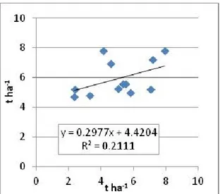
Indices in table 3 confirm the difficulty encountered in the calibration process for ryegrass, indeed RRMSE, EF, MAE, CD were not close to their optimal values. The same result was obtained by the regression analysis (figure 6) where the value of the coefficients of the regression line (intercept: 4.42; slope: 0.30 and R2: 0.21), between observed and simulated data confirm the inaccurately yield simulation considering all the treatments.

Figue 6:Observed annual forage yield vs yield simulated by EPIC.

Table 3: Statistical indices to assess simulation efficiency after the calibration.

Parameter MAE RRMSE EF CRM CD

Min 0.00 0.00 -inf. -inf. 0.00

Max +inf. +inf. 1.00 +inf. +inf.

Best 0.00 0.00 1.00 0.00 1.00

Calculated value 1.33 35.47 -0.07 -0.17 1.50

To assess the reason of the lack of precision in the yield simulation for ryegrass, the statistical analysis for single treatments were carried out. The statistical analysis of the results for each treatment shown different results with R2 values that goes from 0.05 for the “slurry” treatment to 0.99 for ”mineral + slurry” treatment.

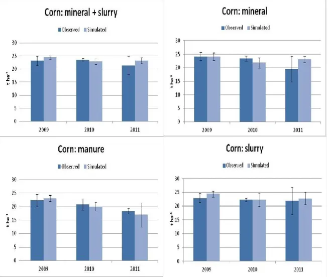
The difficulty in the calibration process for the ryegrass can be partially ascribed to the high variability observed in the measured data within year and within treatments. The worst results were obtained for the “slurry” treatment where the model highly overestimate the actual productions (figure: 7.IV and table: 4.IV). Better results were

obtained for the “manure” and “mineral” treatments where for manure a good R2

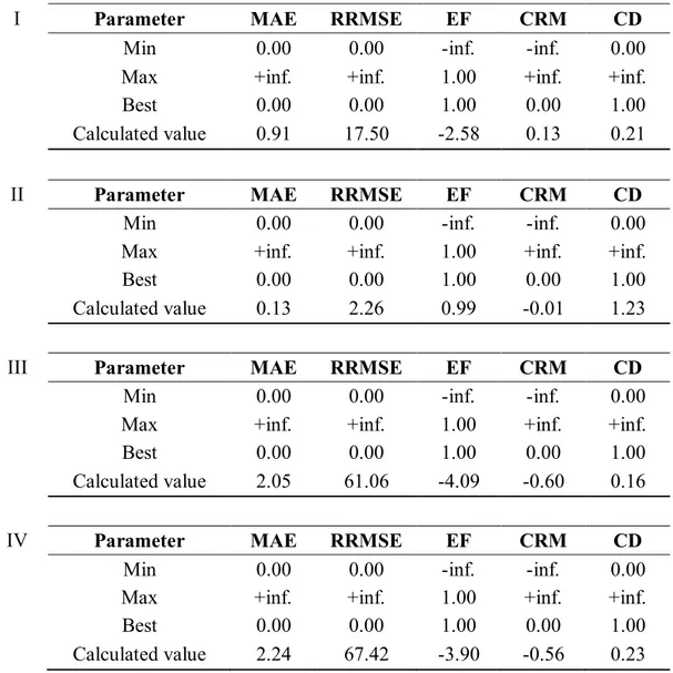
value of 0.85 was obtained thanks to the ability of the model to reproduce the trend of the productions during the experiment despite its systematically overestimation of the ryegrass yields (figure 7.III and table: 4.III); while for the mineral treatment the R2 values was of 0.41. This result was influenced by the high variability observed in the measured yield of different plots in the first and third years (figure: 7.I and table: 7.I). The better result was obtained for the “slurry + mineral” treatment that was used as main driver for the calibration process (R2: 0.99; slope: 0.90; intercept: 0.66) (figure: 7.II and table: 4.II).

Figure 7: Observed annual forage yield vs yield simulated by EPIC. I) “mineral” treatment, II) “mineral + slurry” treatment, III) “manure” treatment, IV) “slurry” treatment.

I II

Table 4: Statistical indices to assess simulation efficiency after the calibration. I) “mineral” treatment, II) “mineral + slurry” treatment, III) “manure” treatment, IV) “slurry” treatment.

I Parameter MAE RRMSE EF CRM CD

Min 0.00 0.00 -inf. -inf. 0.00

Max +inf. +inf. 1.00 +inf. +inf.

Best 0.00 0.00 1.00 0.00 1.00

Calculated value 0.91 17.50 -2.58 0.13 0.21

II Parameter MAE RRMSE EF CRM CD

Min 0.00 0.00 -inf. -inf. 0.00

Max +inf. +inf. 1.00 +inf. +inf.

Best 0.00 0.00 1.00 0.00 1.00

Calculated value 0.13 2.26 0.99 -0.01 1.23

III Parameter MAE RRMSE EF CRM CD

Min 0.00 0.00 -inf. -inf. 0.00

Max +inf. +inf. 1.00 +inf. +inf.

Best 0.00 0.00 1.00 0.00 1.00

Calculated value 2.05 61.06 -4.09 -0.60 0.16

IV Parameter MAE RRMSE EF CRM CD

Min 0.00 0.00 -inf. -inf. 0.00

Max +inf. +inf. 1.00 +inf. +inf.

Best 0.00 0.00 1.00 0.00 1.00

3.2.Climatic scenarios simulation results

The result of the calibration activity allowed, with a reasonable accuracy, the application of the EPIC model for a simulations exercise in this climatic scenarios. The simulations performed with synthetic present and future climate scenarios, allowed the evaluation of the possible response of the studied system to a change in the climate condition.

Figure 8 shows the frequency distribution of the yields of ryegrass related to “mineral+slurry” treatment, which showed for the future climates (CF_380 and CF_407) a reduction of variability.

Figure. 8: Frequency distribution of the yields of Italian ryegrass related to treatment mineral+slurry for the 3 selected climate scenario.

Table 5: Mean Italian ryegrass hay production (t ha-1 _{DM) as influenced by the tested climate}

scenarios.

CP_YLDF vs CF_380_YLDF CF_380_YLDF vs CF_407_YLDF

Average 5.91 A 5.88 A 5.88 A 5.95 A

S.D. 1.05 0.73 0.73 0.76

C.V. 17.74% 12.43% 12.43% 12.79%

With regard to the frequency distribution of corn yields (figure 9) shows a very similar trend in all the synthetic scenarios, the displacements of the curve are due to the different average production; which results to be statistically different for α of 0.05 for the three different scenarios (table 6).

Figure 9: Frequency distribution of corn yields related to treatment mineral+slurry for 3 selected climate scenario.

Table 6: Mean silage corn yield (t ha-1 _{DM) as influenced by the tested climate scenarios.}

CP_YLDF vs CF_380_YLDF CF_380_YLDF CF_407_YLDF

Average 22.90 A 23.42 B 23.42 A 23.76 B

S.D. 0.69 0.73 0.73 0.73

C.V. 3.03% 3.10% 3.10% 3.07%

The simulation of treatment “Mineral” for ryegrass (figure 10) showed a frequency distribution of yields with higher frequencies in correspondence of the higher average yields for the two future scenarios compared to the present climate, that also presents a greater variability.

The average yield of the three scenarios do not differ statistically for α 0.05 (table 7).

Figure 10: Frequency distribution of the yields of Italian ryegrass related to treatment mineral for 3 selected climate scenario.

Table 7: Mean Italian ryegrass hay production (t ha-1 _{DM) as influenced by the tested climate}

scenarios.

CP_YLDF vs CF_380_YLDF CF_380_YLDF vs CF_407_YLDF

Average 5.93 A 5.94 A 5.94 A 6.01 A

S.D. 1.11 0.76 0.76 0.77

C.V. 18.78% 12.76% 12.76% 12.77%

The yields of corn silage in future climate, for treatment “Mineral”, were on average higher than those in the present climate due to its higher frequency of low productions. The yields of the three scenarios differ statistically for α 0.05 (figure 11, table 8).

Figure 11: Frequency distribution of the yields of corn related to treatment mineral for 3 selected climate scenario.

Table 8: Mean corn silage yield (t ha-1 _{DM) as influenced by the tested climate scenarios.}

CP_YLDF vs CF_380_YLDF CF_380_YLDF vs CF_407_YLDF

Average 21.49 A 21.78 B 21.78 A 22.08 B

S.D. 76.26 0.77 0.77 0.82

C.V. 3.20% 3.53% 3.53% 3.71%

In the simulations of the “Manure” treatment, the frequency distribution of the yields of hay ryegrass shows for the two future scenarios an average production lower than in present climate (figure 12). The productions of all the scenarios does not statistically differ for α 0.05 (table 9).

Figure 12: Frequency distribution of the yields of Italian ryegrass related to treatment manure for 3 selected climate scenario.

Table 9: Mean Italian ryegrass hay production (t ha-1 _{DM) as influenced by the tested climate}

scenarios.

CP_YLDF vs CF_380_YLDF CF_380_YLDF vs CF_407_YLDF

Average 3.61 A 3.30 B 3.30 A 3.34 A

S.D. 0.70 0.65 0.65 0.67

C.V. 19.29% 19.70% 19.70% 20.19%

For corn with “Manure” treatment, the frequency distribution of yields for the three climate scenarios shown an extremely high variability with high frequency of yields higher than the average values and at the same time a high percentage of yield lower than the average values. The yields relative to the CP and CF_380 are not statistically different, while CF_407 differ statistically for α 0.05 (figure 13, table 10).

Figure 13: Frequency distribution of corn yields related to treatment manure for 3 selected climate scenario.

Tabella 10: Mean silage corn yield (t ha-1 _{DM) as influenced by the tested climate scenarios.}

CP_YLDF vs CF_380_YLDF CF_380_YLDF vs CF_407_YLDF

Average 16.04 A 16.46 A 16.46 A 17.87 B

S.D. 4.21 4.31 4.31 4.18

C.V. 26.26% 26.20% 26.20% 23.38%

The ryegrass “Slurry” treatment, shows a frequency distribution of yields almost identical for the CF_380 and CF_407 and compared with the CP, less variability; yields for CP statistically differ from CF_380 and CF_407 for α 0.05, while yields obtained with future scenarios do not statistically differ for α 0.05 (figure 14, table 11).

Figure 14: Frequency distribution of the yields of Italian ryegrass related to treatment slurry for 3 selected climate scenario.

Table 11: Mean Italian ryegrass hay production (t ha-1 _{DM) as influenced by the tested climate}

scenarios.

CP_YLDF vs CF_380_YLDF CF_380_YLDF vs CF_407_YLDF

Average 5.85 A 6.08 B 6.08 A 6.18 A

S.D. 0.78 0.59 0.59 0.62

C.V. 13.29% 9.64% 9.64% 10.08%

In the simulation of corn for the “Slurry” treatment, the frequency distribution shows that in future climates high yields may occur more frequently. Yields between present and future climate statistically differ for α 0.05, while among CF_380 and CF_407 there are no statistically significant differences for α 0.05 (figure 15, table 12).

Figure 15: Frequency distribution of the yields of corn related to treatment slurry for 3 selected climate scenario.

Table 12: Mean silage corn yield (t ha-1 _{DM) as influenced by the tested climate scenarios.}

CP_YLDF vs CF_380_YLDF CF_380_YLDF vs CF_407_YLDF

Average 20.28 A 20.68 B 20.68 A 20.84 A

S.D. 1.14 0.95 0.95 0.98

C.V. 5.61% 4.60% 4.60% 4.73%

By simulations carried out with the same crop management observed during the trial we obtained relevant information on the potential impacts of the tested climate scenarios .

Considering that the crop yield for annual crops is estimated by EPIC using the harvest index concept, which is adjusted throughout the growing season according to growth constraints, and that the physiological responses to water stress is considered with direct impact on harvest index and canopy growth several simulations with different managements were carried out.

In the studied area the plants water requirement is satisfy by the sum of precipitation and irrigation, and by the groundwater table uptake. To quantify the contribution of the groundwater table a simulation without water table was carried out. The result was a reduction of yield in all the climates tested. Regarding the ryegrass yield reductions for the CP was 30%, 26% in CF_380 while in CF_407 the reduction was 25%. The yields were also lower for corn: 43% in the CP, 47% in CF_380 and 46% in CF_407.

The average number of days of water stress for ryegrass with the CP scenario and with the groundwater table was 9 (SD 4), while without the groundwater table it increase to 35 (SD 14) days of stress. Moreover, the growing season evapotranspiration (GSET) decreases by 26%. In the CF_380 scenario with water table the average number of days of water stress for ryegrass was 11 (SD 4), while in absence of groundwater table, the days of stress rise to 42 (SD 15), and the GSET degrease of 31%. In the CF_407 scenario with groundwater table the average number of days of water stress were 10 (SD 4), and in the absence of ground water the days of stress were 41 (SD 15) and GSET by 30%. For corn, the CP scenario with the groundwater table has on average 3 (SD 0.8) days of water stress, while in absence of groundwater table has on average 42 (SD 4) days of stress and GSET decreases by 45%. In the CF_380 scenario with the water table the days of water stress were on average 4 (SD 0.7), while without the groundwater table, the days of stress were 46 (SD 4) and GSET degrease of 49%. In the CF_407 scenario with the water table the days of stress were 4 (SD 0.7), and in absence of the water table were 46 (SD 4), the GSET decrease by 49%.

Table 13: Variation in number of days of water stress (WS), growing season evapotranspiration (GSET, mm) for ryegrass with the different climate scenarios.

CP CF_380 CF_407 With water t. Without water t. With water t. Without water t. With water t. Without water t. WS 9±4 35±14 11±4 42±15 11±4 41±15 GSET 379±53 280±37 412±50 286±37 408±49 285±37

Table 14: Variation in number of days of water stress (WS), growing season evapotranspiration (GSET, mm) for corn with the different climate scenarios.

CP CF_380 CF_407 With water t. Without water t. With water t. Without water t. With water t. Without water t. WS 3±1 42±4 4±1 46±4 4±1 46±4 GSET 691±34 378±20 744±35 377±18 733±35 377±18

Conducing simulation without the groundwater table and eliminating the water stress using the automatic irrigation option in EPIC we were able to quantify the irrigation volumes required to ensure the observed yields and, at the same time, the contribution of the water provided by the water table.

For ryegrass with the CP scenario and with the water table the simulated average annual irrigation water applied was 223 mm. In simulations carried out without the water table the irrigation water applied increased by 56%. The same comparison were performed for simulation based on the future scenarios and rise of the irrigation water applied was higher compared with the CP scenario: 113% and 114% for CF_380 and CF_407 respectively.

The same analysis were performed also for corn. With CP scenario and without water table irrigation volume was higher than with water table (122%). In future scenarios and without water table the irrigation volume increased by 126% for CF_380 and by 127% for CF_407 scenario (figure 15, figure 16).

Figure 16: Irrigation water automatically applied by the EPIC model for Italian ryegrass in simulations with and without groundwater table.

Figure 17: Irrigation water automatically applied by the EPIC model for corn in simulations with and without groundwater table

To assess the impacts of CC on the studied cropping system a simulation derived by the “business as usual” situation were performed. The simulation was characterized by automatic irrigation and fertilization to eliminate water and nitrogen stress, absence of the groundwater table, fixed sowing and harvesting dates based on the dates observed during the three years trial.

Comparing the different climate scenarios, the outputs of the simulation shows an increase of the ryegrass yield of 10% and 14% for CF_380 and CF_407 respectively. At the same time the irrigation volumes in the future scenarios increase by 9% in CF_380 and by 8% in CF_407. The same results were obtained for corn where the average yield in the future scenarios increase of 2% in CF_380 and of 3% for CF_407. Again, the irrigation volumes in future scenarios where higher compared with the present scenario (10% for CF_380 and 9% for CF_407).

In order to assess the impacts of the CC on the phenology we checked the heat units accumulated by the crops during their growing seasons (HU). With fixed planting and harvesting dates, the HU accumulated at harvest by the ryegrass in the future scenario were lower by 11% compared to the present scenario, while for maize the HU increase by 10%.

In a second step the same simulation was performed using variable dates for planting and harvest operation. The dates were estimated by the model according to the heat units of the year for sowing operation and to the heat units accumulated by the crop for the harvest operation. HUI-based crop management is also found to be a satisfactory substitute of field-observations (Niu et al., 2009).

Thanks to this simulation we were able to assess the variation of the length of the growing season comparing the results obtained with CP against CF scenarios. The outputs shows that with the future scenarios the growing season was 8 days longer for the ryegrass, while the corn cycle decreases of 9 days. Then, the effect on yields of the modification of growing season was observed and the results for fixed and variable dates within climate scenario were compared. For CP the ryegrass yield increased by 14% from fixed to variable dates, while for CF the yields increase by 5% and 6% with 380 and 407 ppm of CO2 respectively. For corn the yields with

variable harvest dates were 3% lower in the CP scenario, and 12% lower in the CF_380 and CF_407 scenarios. At the same time for the CP scenario the irrigation

volumes for ryegrass increased by 17% from fixed to variable harvest dates, and were 14% and 13% higher in CF_380 and CF_407 scenarios.

Comparing the yields obtained by the simulations with variable sowing and harvest dates for CP and CF scenarios emerged that the ryegrass yield in the CF_380 scenario increased by 35% and the water consumption increased by 49%, while for corn the yield was reduced by 8% and water consumption increased by 1%.

To simulate the adoption of different varieties as adaptation strategy, the number of heat units required by the crops to reach the physiologic maturity (PHU) was modified.

Adopting the adaptation strategy for ryegrass we obtain a slight yield reduction (from +35% to +29%) and at the same time a reduction of water consumption that goes from +49% without adaptation strategy to +40% modifying the ryegrass PHU. For corn yields decreased only by 2% compared with the -8% obtained without adaptation strategy, with an increase of the irrigation volumes by 6%. The ryegrass yields variation can be ascribed to the reduction of the numbers of days of temperature stress which goes from 33 to 26, and at the same time an increased number of days of water stress (from 15 to 18). Corn does not show a large reduction of days of temperature stress, which become 3 starting from 4, while the days of water stress increases from 1 to 2 in spite of the increased irrigation volume applied.

Figure 19: Variation in the number of days of water stress, temperature stress and yield in corn with the modified value of PHU as adaptation strategy.

4. Discussion

This research has presented a modeling approach for the analysis of vulnerability to climate change of a corn-ryegrass forage system in Mediterranean area.

In Mediterranean countries, cereal crops are limited by water availability, thermal stress and the short duration of grain filling period, and the irrigation management is important for crop production due to the high evapotranspiration and limited rainfall. The simulations carried out based of the conditions observed during the trial provide irrigation volumes of 462 ± 22 mm for corn and 75 ± 41 mm for ryegrass.

The study carried out by Giola et al., (2012) in the same studied area report irrigation volumes of 600 mm for maize, and simulated yield of 22.9 t ha-1_{, and is in line with}

the yields simulated by EPIC in the “business as usual” “mineral+slurry” treatment. Simulations without groundwater table, caused poor crop growth and low yields. According to Barron et al. (2003), short periods of water stress that occur during critical water sensitive development stages of crop have significant effect on crop growth and yields. In agreement with Ficklin et al., (2010) it was assumed that to

maintain peak crop production, growers would irrigate so that the crop was rarely under water stress. Since groundwater recharge is a direct result of irrigation water use during growing months, the assumption that the plant will achieve maximum growth due to unlimited water from water table may distort the results.

Without groundwater, irrigation volumes differ on average of 393 mm for corn and 127 mm for ryegrass, without water stress in the CP scenario.

Although irrigation may be beneficial in mitigating the impacts of drought on yield, increased water uptake may have negative impacts that may include increased groundwater depletion, increased water supply costs and lower water availability for other uses. Careful policy will ensuring a minimal impact on water resources. The economic benefit that is derived from supplemental irrigation in hot summers, or when droughts occur, should be carefully weighed against environmental impacts (van der Velde et al., 2010).

4.1.Impacts of CC: automatic irrigation and fertilization, fixed sowing and harvesting dates

The results showed common trends for both the future scenarios over the present scenario: increase of maize and ryegrass biomass production, increase of ET and increase of irrigation volumes.

According to Reidsma et al., (2010), which shows the analysis comparing spatial yield variability in simulated and actual maize yields showed that higher temperatures tend to increase actual yields compared to potential yields. Also the temporal analysis of yield variability indicated that in Mediterranean regions higher temperatures had a more positive impact on actual yields than on the simulated potential yields.

In the future scenario with 407 ppm of CO2 the productions are higher compared with

the scenario with 380 ppm CO2, as illustrated in the study of Leakey et al., (2009) the

increase in atmospheric concentrations of CO2 would drive larger accumulation of

biomass.

About the use of water for crops production, the study of Liu (2013) shows that climate change will alter the magnitude of this variable and also the final aggregate

AWI value .At the continental level, in the 2030s lower the aggregated consumptive water use index (AIWI) occurs with a high level of confidence in all continents except for Europe which has no clear trend of increase or decrease. For Europe, lower total amount of consumptive water use for the representative crops, occurs in six out of eight scenarios; one possible reason for the lower AWI could be that higher CO2

concentration reduces crop stomatal closure thus decreases actual crop ET by reducing plant traspiration.

5. Conclusions

The work has involved the study of two different forage systems and the impact of climate change on them through the use of the simulation model EPIC.

The model calibration gave satisfactory results, as demonstrated by statistical indices used even if some problems were encountered in the calibration for ryegrass where the model has not been able to simulate the observed low production simulating, on the contrary, a high biomass production due to an excessive mineralization of stable organic matter. However, the calibration data acquired from the field experiment allowed a satisfactory simulation of crops growth, highlighting their sensitivity to different environmental conditions. The results of the simulations carried out to assess the impact of climate change show that the climate change could affect the crops productions modifying average yields and yields distribution, the amount of water evapotranspirated during the crop cycle and the number of day with water stress. The simulated adaptation strategy leads to a reduction in the number of days with water stress and in the water consumption. The projections of the impact and risk obtained must be interpreted considering the difficulties inherent in the use of a simulation model in a complex agro-ecosystem with some extreme features such as the Arborea site.

6. References

Aiawort E.A., Long S.P., 2005. What have we learned from 15 years of free-air CO2

enrichment (FACE)? A meta-analytic review of the responses of photosynthesis, canopy properties and plant production to rising CO2. New Phytol. 165: 351–372.

Allen Jr., L.H., Kakani V.G., Vu J.C.V., Boote K.J., 2011. Elevated CO2 increases water use efficiency by sustaining photosynthesis of water-limited maize and sorghum. Kournal Plant Physiol 168 ,1909–1918.

Araus J.L., Slafer G.A., Royo C., Serret M.D., 2008. Breeding for yield potential and stress adaptation in cereals. CRC Crit. Rev. Plant Sci. 27 (6), 377–412.

Barron, J., Rockström, J., Gichuki, F., Hatibu, N., 2003. Dry spell analysis and maize yields for two semi-arid locations in east Africa. Agricultural and Forest Meteorology 117, 23–37.

Barros I, Williams J.R., Gaiser T., 2004. Modeling soil nutrient limitations to crop production in semiarid NE of Brazil with a modified EPIC version I. Changes in the source code of the model. Ecological Modelling 178, 441–456.

Bellocchi G., Donatelli M., Monotti M., Carnevali G., Corbellini M., Scudellari D., 2006. Balance sheet method assessment for nitrogen fertilization in winter wheat: II. Alternative strategies using the CropSyst simulation model. Ital. J. Agron. 1 (3), 343–357.

Bellocchi G., Rivington M, Donatelli M., Matthews K., 2010. Validation of biophysical models: issues and methodologies. A review. Agron. Sustain. Dev. 30. 109–130.

Bellocchi, G., Donatelli, M., Monotti, M., Carnevali, G., Corbellini, M., Scudellari, D., 2006. Balance sheet method assessment for nitrogen fertilization in winter wheat: II. Alternative

Brown, R.A., Rosenberg, N.J., 1997. Sensitivity of crop yield and water use to change in a range of climatic factors and CO, concentrations: a simulation study applying EPIC to the central USA. Agricultural and Forest Meteorology 83, 171– 203.

Campos H., Cooper M., Habben J.E., Edmeades G.O., Schussler J.R., 2004. Improving drought tolerance in maize: a view from industry. Field Crops Res. 90 (1), 19–34.

Chavas D.R., Izaurralde R.C., Thompson A.M., Gao X., 2009. Long-term climate change impacts on agricultural productivity in eastern China. Agric. For. Meteorol. 149 (6–7), 1118–1128.

Costantini, E.A.C, Bocci, M., L’Abate, G., Fais, A., Leone, G., Loj, G., Magini, S., Napoli, R., Nino, P., Urbano, F., 2004. Mapping the state and risk of desertification in Italy by means of remote sensing, soil GIS and the EPIC model. methodology validation in the Sardinia island, Italy. International Symposium: Evaluation and Monitoring of Desertification. Synthetic Activities for the Contribution to UNCCD, Tsukuba, Ibaraki, Japan, February 2 2004, NIES publication.

De Sanctis G., Lai R., Demurtas C., Gennaro L., Ledda L., Seddaiu G., Roggero P.P., 2011. Gestione Irrigua su Sistemi Colturali Maidicoli in Zona Vulnerabile da Nitrati della Provincia di Oristano. In: M. Pisante and F. Stagnari (eds.) Atti XL Convegno SIA Teramo, Italy, 354-355.

Dhakhwa G.B., Campbell C.L., LeDuc S.K., Cooter E.J., 1997. Maize growth: assessing the effects of global warming and CO2 fertilization with crop models. Agric. For. Meteorol. 87, 253–272.

Diffenbaugh N.S., Field C.B., 2013. Review Changes in Ecologically Critical Terrestrial Climate Conditions. Science: Vol. 341 no. 6145 pp. 486-492 DOI: 10.1126/science.1237123

Doraiswamy, P.C., McCarty, G.W., Hunt, E.R. Jr., Yost, R.S., Doumbia, M., Franzluebbers, A.J., 2007. Agricultural Systems 94, 63–74.

Easterling W.E., Chen X., Hays C., Brandle G.R., Zhang H., 1996. Improving the validation of model-simulated crop yield response to climate change: an application to the EPIC model. CLIMATE RESEARCH 6: 263–273.

Eitzinger J., Stastná M., Zalud Z., Dubrovsky´ M., 2003. A simulation study of the effect of soil water balance and water stress on winter wheat production under different climate change scenarios. Agric. Water Manage. 6 (3), 195–217.

Falloon P., Betts R., 2010. Climate impacts on European agriculture and water management in the context of adaptation and mitigation — The importance of an integrated approach. Science of the Total Environment 408, 5667–5687.

Ficklin D. L., Luedelinga E., Zhanga M., 2010. Sensitivity of groundwater recharge under irrigated agriculture to changes in climate, CO2 concentrations and canopy

structure. Agricultural Water Management 97, 1039–1050.

Finger L.R., Klein T., Calanca P., Niklaus W. A., 2013. Adapting crop management practices to climate change: Modeling optimal solutions at the field scale.. Agricultural Systems 117, 55–65.

Fuhrer J., 2003. Agroecosystem response to combinations of elevated CO2, ozone,

and global climate change. Agr. Ecosyst. Environ. 97, 120.

Giola P., Basso B., Pruneddu G., Giunta F., Jonens J.W., 2012. Impact of manure and slurry applications on soil nitrate in a maize–triticale rotation: Field study and long term simulation analysis. European Journal of Agronomy,38, 43–53.

Goubanova K., Li L., 2006. Extremes in temperature and precipitation around the Mediterranean in an ensemble of future climate scenario simulations. Global Planet. Change. http://dx.doi.org/10.1016/j.globaplacha.2006.11.012.

Granta R.F., Baldocchi D.D. , Mab S., 2012. Ecological controls on net ecosystem productivity of a seasonally dry annual grassland under current and future climates: Modelling with ecosys. Agricultural and Forest Meteorology 152, 189– 200.

Guerena A., Ruiz-Ramos M., Diaz-Ambrona C.H., Conde J.R., Minguez M.I., 2001. Assessment of climate change and agriculture in Spain using climate models. Agron. J. 93 (1), 237–249.

Guo R., Lin Z., Mo X., Yang C., 2010. Response of crop yield and water use efficiency to climate change in the North China Plain. Agric. Water Manag. 97, 1185–1194.

Haskett J.D., Pachepsky Y.A., Acock, B., 1997. Increase of CO2 and climate change effects on Iowa soybean yield, simulated using GLYCIM. Agron. J. 89 (2), 167– 176.

IPCC, 2007. Climate Change 2007: Synthesis Report.

Izaurralde, R.C., Williams, J.R., McGill, W.B., Rosenberg, N.J., Quiroga Jakas, M.C., 2007. Long-term modeling of soil C erosion and sequestration at the small watershed scale. Climatic Change, 80, 73–90.

Jones P.G., Thornton P.K., 2003. The potential impacts of climate change on maize production in Africa and Latin America in 2055. Global Environ. Change 13 (1), 51–59.

Jørgensen, S.E., Kamp-Nielsen, L., Christensen, T., Windolf-Nielsen, J., We stergaard, B., 1986. Validation of a prognosis based upon a eutrophication model. Ecol. Modell. 32, 165-182.Liu J, Folberth C.,Yang H., Rockstrom J., Abbaspour K., Zehnder A.J.B., 2013. A Global and Spatially Explicit Assessment of Climate Change Impacts on Crop Production and Consumptive Water Use. PLOS ONE. Volume 8 | Issue 2 | e57750.

Kemanian A.R., Stöckle C.O., Huggins D.R., 2004. Variability of Barley Radiation-Use Efficiency. Crop Sci. 44:1162–1173.

Kimball B.A., Kobayashi K., Bindi M., 2002. Responses of agricultural crops to freeair CO2 enrichment. Adv. Agron. 77, 293–368.

Kriegler E., O’Neill B.C., HallegatteS., Kram T., Lempert R.J., Moss R.H., WilbanksT., 2012.The need for and use of socio-economic scenarios for climate change analysis: A new approach based on shared socio-economic pathways. Global Environmental Change 22, 807–822.

Leakey A.D.B., 2009. Rising atmospheric carbon dioxide concentration and the future of C4 crops for food and fuel. Proc. R. Soc. B 276, 2333–2343.

Lehmann N., Finger R., Klein T., 2011. Optimizing Wheat Management Towards Climate Change: A Genetic Algorithms Approach. In: IASTED International Conference on Applied Simulation and Modelling, 22–24 June 2011, Crete, Greece. Lehmann N., Finger R., Klein T., Calanca P., Walter A., 2013. Adapting crop

management practices to climate change: Modeling optimal solutions at the field scale. Agricultural Systems 117, 55–65.

Liu J., Williams J.R., Zehnder A.J.B., Yang H., 2007. GEPIC—modelling wheat yield and crop water productivity with high resolution on a global scale. Agric. Syst. 94, 478–493.

Lovelli S., Perniol, M., Di Tommaso T., Ventrella D., Moriondo M., Amato M., 2010. Effects of rising atmospheric CO2 on crop evapotranspiration in a Mediterranean area. Agric. Water Manag. 97, 1287–1292.

Merot A., Bergez J.E. , Wallach D., Duru M., 2008. Adaptation of a functional model of grassland to simulate the behaviour of irrigated grasslands under a Mediterranean climate: The Crau case. Europ. J. Agronomy 29, 163–174.

Naudtsa K. , Van den Bergea J. , Janssensa I.A. , Nijs I., Ceulemansa R., 2011. Does an extreme drought event alter the response of grassland communities to a changing climate?. Environmental and Experimental Botany 70, 151–157.

Niu X., Easterling W., Hays C.J., Jacobs A., Mearns L., 2009. Reliability and input-data induced uncertainty of the EPIC model to estimate climate change impact on sorghum yields in the U.S. Great Plains. Agriculture, Ecosystems and Environment 129, 268–276.

OECD, 2006. Report on the OECD Workshop on Agriculture and Water: Sustainability, Markets and Policies, Adelaide, Australia, 14–18 November 2005, COM/AGR/CA/ENV/EPOC/RD, 2005, pp. 71.

Olesen J.E., Bindi M. 2002. Consequences of climate change for European agricultural productivity, land use and policy. European Journal of Agronomy, 16, 239-262.

Olesen J.E., Trnka M., Kersebaum K.C., Skjelvåg A.O., Seguin B., Peltonen-Sainio P., Rossi F., Kozyra J., Micale F., 2011. Impacts and adaptation of European crop production systems to climate change. Europ. J. Agronomy 34, 96–112.

Porter J.R., Semenov M.A., 2005. Crop responses to climatic variation. Philos T Royal Soc B 360:2021–2035.

Reidsma P., Ewert F., Lansink A.O., Leemans R., 2010. Adaptation to climate change and climate variability in European agriculture: The importance of farm level responses. Europ. J. Agronomy 32: 91–102.

Rinaldi M., D’Andrea L., Ruggieri S., Garofalo P. Moriondo M. Ventrella D., 2009. Influenza dei cambiamenti climatici sulla coltivazione del frumento duro. Atti Convegno Nazionale Società Italiana di Agrometereologia, 2:32–33.

Rodriguez Diaz J.A., Weatherhead E.K., Knox J.W., Camacho E., 2007. Climate change impacts on irrigation water requirements in the Guadalquivir river basin in Spain. Regional Environ. Change 7, 149–159.

Rosenzweig C., Parry M.L., 1994. Potential impact of climate change on world food supply. Nature 367, 133–138.

Rosenzweig, C., Hillel, D., 1998. Climate Change and the Global Harvest. Oxford University Press, Oxford, UK.

Saxton, K.E., Willey, P.H., 2006. The SPAW model for agricultural field and pond hydrologic simulation. In Watersheds Models, V.P. Singh, D.K. Frevert. CRC Press.

Soussana J.F., Graux A.I, and Tubiello F.N., 2010. REVIEW PAPER Improving the use of modelling for projections of climate change impacts on crops and pastures. Journal of Experimental Botany, Vol. 61, No. 8, 2217–2228.

Stöckle C. O. and J. R. Kiniry. 1990. Variability in crop radiation use efficiency associated with vapor pressure deficit. Field Crops Research 25:171-181.

Tan G., Shibasaki R., 2003. Global estimation of crop productivity and the impacts of global warming by GIS and EPIC integration. Ecol. Model. 168: 357–370.

Tingem M., Rivington M., 2009. Adaptation for crop agriculture to climate change in Cameroon: turing on the heat. Mitig. Adapt. Strategies Glo. Chang. 14: 153–168. Torriani D.S., Calanca P., Lips M., Ammann H., Beniston M., Fuhrer J., 2007a.

Regional assessment of climate change impacts on maize productivity and associated production risk in Switzerland. Reg. Environ. Change 7, 209–221.

Torriani D.S., Calanca P., Schmid S., Beniston M., Fuhrer J., 2007b. Potential effects of changes in mean climate and climate variability on the yield of winter and spring crops in Switzerland. Clim. Res. 34 (1), 59–69.

Tubiello F., Donatelli M., Rosenzweig C., Stockle C.O., 2000. Effects of climate change and elevated CO2 on cropping systems: model predictions at two Italian locations Francesco N., Marcello, C. Claudio O.. European Journal of Agronomy 13, 179–189.

Tubiello F.N., DonatelliM., Rosenzweig C., Stockle C.O., 2000. Effects of climate change and elevated CO2 on cropping systems: model predictions at two Italian

locations. European Journal of Agronomy 13: 179–189.

Tubiello FN, Donatelli M, Rosenzweig C, Stöckle CO (2000) Effects of climate change and elevated CO2 on cropping systems: model predictions at two Italian