Effects of meteorology on PM10 concentrations: a comparative assessment of machine learning methods

Alma Mater Studiorum · Universit`

a di Bologna

Scuola di Scienze

Dipartimento di Fisica e Astronomia Corso di Laurea Magistrale in Fisica

Effects of meteorology on PM

₁₀

concentrations: a comparative assessment

of machine learning methods

Relatore:

Prof. Gastone Castellani

Correlatrice:

Prof.ssa Claudia Sala

Presentata da:

Davide Ferraresi

Contents

1 Introduction 7

1.1 Air quality and pollution . . . 9

1.1.1 Air pollutants and main sources of emissions . . . 9

1.1.2 Geographical variability and concentration monitoring . . . 10

1.1.3 International policies . . . 12

1.2 Particulate matter (PM) . . . 13

1.2.1 Effects on human health . . . 15

1.2.2 Legal thresholds and guideline values for concentration . . . 16

1.2.3 Emission and concentration monitoring . . . 17

1.3 Context overview: Emilia-Romagna . . . 23

1.3.1 Geographical and meteorological elements . . . 23

1.3.2 Anthropic pression and emission sources . . . 24

1.3.3 Air quality and meteorology . . . 25

1.3.4 Regional concentration monitoring . . . 25

1.4 Models for PM10 prediction . . . 29

1.4.1 Previous works on PM₁₀ forecasting . . . 32

1.4.2 Previous works on other pollutants’ forecasting . . . 32

1.4.3 Some remarks . . . 35

2 Materials and methods 36 2.1 Data overview and exploratory analysis . . . 36

2.1.1 EDA techniques . . . 38

2.1.2 Particulate Matter concentration . . . 42

2.1.3 Temperature . . . 51

2.1.4 Precipitation . . . 55

2.1.5 Wind intensity and direction . . . 58

2.1.6 Radiant exposure . . . 65

2.1.7 Atmospheric pressure . . . 67

2.1.8 Mixed layer height . . . 69

2.2 Missing data treatment and imputation . . . 72

2.2.2 Multiple imputation of missing data . . . 73

2.3 Linear regression models . . . 74

2.3.1 Standard linear regression . . . 75

2.3.2 Ridge regression . . . 76

2.3.3 Lasso regression . . . 77

2.4 Regression tree models . . . 77

2.4.1 Bagging and random forests . . . 79

2.4.2 Boosting . . . 80

2.5 Model assessment and selection . . . 81

2.5.1 Measuring the error . . . 81

2.5.2 Choosing the predictors . . . 82

2.5.3 Splitting the datasets . . . 82

2.5.4 Cross-validation procedure . . . 83

2.5.5 Model selection and assessment of the performances . . . 84

2.5.6 Classification task based on PM10 daily limit value . . . 86

2.5.7 Approach with MI datasets . . . 86

2.6 Implementation in R . . . 88

2.6.1 Missing data treatment and imputation . . . 88

2.6.2 Linear regression models . . . 91

2.6.3 Regression tree models . . . 92

2.6.4 Cross-validation, model selection and comparison . . . 92

2.6.5 Classification task . . . 93

3 Results 95 3.1 Performance on LWD-basic datasets . . . 95

3.2 Comparison of performances on LWD-basic and MI-basic datasets . . . . 98

3.3 Performance of models with non-meteorological predictors . . . 99

3.4 Comparing models for classification tasks . . . 101

4 Conclusions 103 4.1 Further developments . . . 104

Abstract

Administrative decisions regarding the application of measures to address air quality issues have to rely both on present observation and future predictions of the concentration of various pollutants. Since PM10 is one of the most critical pollutants, the ability to

provide accurate forecasts for its concentration, when required, is crucial in order to enforce the necessary measures at the right time.

Together with the pattern of emission sources which is present in a geographical area, meteorological conditions can significantly affect the concentration of pollutants in air, since they can favour the dispersion or, on the other hand, the build-up of those com-pounds. It is possible then to predict (at least partially) the concentration of PM10 in

air using meteorological variables as predictors.

In fact, various statistical models have been proposed for accomplishing similar tasks on a number of geographical regions and urban areas, with varying results. The set of mete-orological variables that have been considered in those cases included various predictors, measured both in the day of interest and in the previous ones. Sometimes also some non-meteorological descriptors (e.g. time-related variables) that are grossly related to the variation of the emission patterns have been considered as input variables for those models.

In this work an analysis of the relationship between meteorology-related variables and PM₁₀ concentration levels in the capitals of the provinces of Emilia-Romagna has been performed in order to understand how the meteorological conditions affect PM10

con-centration. Then the considered meteorological variables have been input as predictors to statistical regression models based on machine learning in order to obtain predictions for the daily mean value of PM10concentration.

Taking a cue from a synthetic indicator defined by the regional agency ARPAE that links meteorological conditions to the building up of PM₁₀, a dataset containing time series of daily values of 10 meteorological variables and those of PM10urban background

concentration for the 10 cities, spanning a time interval of 2008 days (5 year and a half), has been initially created. Data have been obtained from the public database available on ARPAE websites and processed using R-based software RStudio.

that has allowed to point out the main features of each variable and its relationship with PM₁₀ concentration, evaluated on a daily basis.

After having adequately pre-processed the data, they have been used to train regression models with the aim of predicting PM₁₀ daily mean concentration values starting from the same-day values of the meteorological variables. All the considered models, which include standard and regularized linear regressions and regression tree-based ones, have been trained separately with the data of each city, in order to reproduce specifically the patterns observed at a local level. At the beginning of the exam of those models, only the meteorological data from the same day for which the prediction has to be made have been fed into the model.

The results show that random forest and boosting models are generally better in the prediction tasks, for all the considered cities.

With respect to predictors, the level of model performance obtained with the chosen set of meteorological variables have been subsequently compared with the performances on the same dataset with the addition of non-meteorological variables such as the day of the week and the month related to each sample, and the previous-day PM10 mean

concentration level, in order to improve the performance initially obtained. Statistical tests have shown that the performance improves significantly in a number of cases with time-related descriptors and in all the cases with the addition of the previous-day PM10

value.

Finally, an evaluation of the ability of the considered models to carry out a good “clas-sification” with respect to the legal limit value for PM10 daily mean concentration has

Abstract

Le decisioni delle autorit`a relative all’applicazione di misure di contrasto al degrado della qualit`a dell’aria devono fondarsi sia su misurazioni effettuate, sia su previsioni per i valori futuri di concentrazione delle sostanze inquinanti. Il PM10`e uno degli inquinanti

pi`u controllati e la capacit`a di fornire previsioni accurate per la sua concentrazione, quando richiesto, `e fondamentale per applicare le misure necessarie al momento giusto. Oltre alla distribuzione e alle caratteristiche delle fonti di emissioni presenti in un’area geografica, un elemento che influenza in modo importante le concentrazioni di inquinanti `

e la meteorologia, dal momento che differenti condizioni meteo possono favorire la dis-persione o, al contrario, l’accumulo di queste sostanze. `E quindi possibile effettuare una previsione della concentrazione di PM10in atmosfera impiegando come predittori alcune

variabili meteorologiche.

In effetti diversi modelli statistici capaci di effettuare simili previsioni sono stati applicati su diverse regioni e aree urbane, con risultati di qualit`a variabile. Gli insiemi di variabili meteorologiche impiegati per quei modelli comprendevano diversi predittori, misurati sia nella giornata d’interesse sia in quelle precedenti. In tali modelli sono state talvolta considerate anche alcune variabili non legate al meteo (ad esempio le variabili temporali) che sono legate ai trend di variazione delle emissioni.

In questa attivit`a `e stata compiuta un’analisi della relazione fra variabili meteorologiche e concentrazioni di PM₁₀nei capoluoghi di provincia dell’Emilia-Romagna, con lo scopo di comprendere in che modo le condizioni meteo influenzano le concentrazioni di parti-colato. In seguito tali variabili sono state utilizzate come predittori all’interno di modelli statistici di regressione basati sul machine learning per effettuare previsioni del valore della concentrazione media giornaliera di PM10.

Prendendo spunto da un indicatore sintetico elaborato dall’agenzia regionale ARPAE per identificare le condizioni meteorologiche che favoriscono l’innalzamento dei livelli di PM10 in atmosfera, `e stato costruito un set di dati contenente le serie storiche dei

valori giornalieri di 10 variabili meteorologiche e della concentrazione di fondo urbano di PM₁₀ per ciascuna delle 10 citt`a considerate; il set di dati copre un intervallo di 2008 giorni (circa 5 anni e mezzo). I dati sono stati estratti dai database pubblici di ARPAE disponibili sul sito dell’agenzia e sono stati elaborati mediante il software RStudio basato

sul linguaggio R.

Una volta costruito il set di dati, questo `e stato sottoposto a un’analisi dati esplorativa per mettere in luce le caratteristiche principali di ciascuna variabile e la relazione fra ognuna di esse e la concentrazione di PM10. In particolare si `e evidenziata la relazione

fra le condizioni meteo e la concentrazione dell’inquinante nella stessa giornata.

Una volta eseguite le necessarie operazioni di preprocessing per rendere fruibili i dati, essi sono stati utilizzati per addestrare modelli di regressione allo scopo di predire il valore della concentrazione media giornaliera di PM10a partire dai valori delle variabili

meteo-rologiche nello stesso giorno. Tutti i modelli considerati, che comprendevano modelli di regressione lineare standard, regolarizzata e modelli basati su alberi di regressione, sono stati addestrati separatamente con i dati di ciascuna citt`a, in modo da poter riprodurre gli andamenti osservati nelle diverse localit`a. Inizialmente la procedura di addestramento dei modelli ha incluso come dati di input solamente i valori delle variabili meteorologiche misurate nello stesso giorno per il quale il modello effettuava la previsione.

I risultati hanno dimostrato che, per quanto riguarda i modelli, le random forest e i boosting models si sono dimostrati i pi`u efficaci in tutte le citt`a considerate.

Sul fronte delle variabili utilizzate come predittori, le prestazioni dei modelli addestrati con le variabili meteorologiche sono state successivamente confrontate con le performance degli stessi modelli addestrati con i set di dati integrati con variabili temporali, quali il giorno della settimana e il mese di campionamento del dato, e il valore della concen-trazione media giornaliera di PM₁₀del giorno precedente, allo scopo di valutare eventuali miglioramenti nell’accuratezza. Si sono osservati miglioramenti significativi in una parte dei modelli quando sono stati addestrati con l’integrazione delle variabili temporali; nel caso dei modelli addestrati con la variabile relativa alla concentrazione di PM₁₀del giorno precedente, l’incremento della qualit`a della predizione `e risultato significativo in tutti i casi considerati.

Da ultimo, si `e valutata l’abilit`a dei modelli considerati nel “classificare” correttamente un set di dati rispetto al valore limite legale della concentrazione media giornaliera di PM₁₀, ottenendo buoni risultati su tutti i modelli considerati.

Chapter 1

Introduction

In this work the issue of air pollution in a number of urban areas of Emilia-Romagna, an administrative region of Italy, has been addressed with respect to the effect of mete-orology on the concentration of pollutants in air.

The considered areas are nowadays affected by serious problems concerning ambient air pollution due to PM10concentrations. Therefore, administrative measures are routinely

enforced in the winter months to try to tackle what is still called a “PM10 emergency”.

Applying those measures for harm reduction is necessary to protect the health of peo-ple and administrative bodies are responsible for the decisional process.[16] Measures are generally applied whenever both pollutant’s concentration in the recent past and forecasts for the following days are above the thresholds that have been defined by the law. So the use of forecasting systems is common and a number of methods has been developed to address this need.

A distinction can be made [5] between numerical and statistical methods. The former ones (both bi- and tridimensional) are able to calculate the concentration of pollutant compounds in a selected area by performing a geospatial simulation, i.e. by geographi-cally determining the sources of emissions, the presence of boundaries and the behaviour of the lower layers of the atmosphere and simulating the chemical and physical processes that happen in the air at different spatial and temporal scales. On the contrary, statisti-cal methods are independent on those processes and analyse statististatisti-cally the relationship between descriptors that approximate the various elements of the context (e.g. meteoro-logical trends, geographical patterns of sources, . . . ). This latter kind of methods is the one that has been considered for the present work.

In this work the focus is on the relationship between the behaviour of meteorological vari-ables and the trends in PM₁₀ concentration. As pollutants build up in the atmosphere, some meteorological events can favour the increase or the reduction of the concentra-tions: for this reason, meteorology-related variables (such as temperature, precipitation

intensity and others) can be used as predictors in the aforementioned statistical models together with other variables that are related to other drivers (e.g. the periodical trend of emissions in a year cycle or in a week).

In the following chapters an analysis of the patterns of meteorological variables mea-sured in all the capitals of the provinces of the region (Piacenza, Parma, Reggio Emilia, Modena, Bologna, Ferrara, Ravenna, Forl`ı, Cesena, Rimini) during the period of time between the 1st _{of October, 2012 and the 31}st _{of March, 2018, and the relationship}

be-tween those variables and the measured values of urban background PM10 daily mean

concentration in the same cities is presented.

This analysis is followed by the evaluation of the performances of a number of statistical regression models based on machine learning techniques that take the meteorological variables measured in each city as input in order to predict the PM10 daily mean

con-centration in the same city.

The present chapter examines the issue of air pollution with particular focus on PM10,

the reasons why it is a current problem during winter months and the monitoring pro-cedures that are currently implemented. Then a description of the geographical context in which measures considered in this work have been taken is made and a review of past works that involved the use of statistical models for similar tasks is made.

In chapter 2 an extensive exploratory data analysis on the considered data is presented, in which the patterns of each meteorological variable and the correlation between those and PM10concentration is performed in order to understand how different meteorological

conditions favour the building-up PM10for each considered cities.

Then a number of the regression models that have been considered is presented: these models have been evaluated in order to select the one that best performs in predicting the value of PM10daily mean concentration for each city starting from the values of the

meteorological variables measured in the same day.

The results of the comparative assessment among the models are presented in chap-ter 3, where the performances of the same models on datasets integrated with non-meteorological variables are also shown.

Conclusions are made in chapter 4, where considerations are made about possible future developments of this work.

1.1

Air quality and pollution

The state of air quality is a current matter of concern, not only for decision makers but for society in general: a European Commission survey [14] has found it is considered as the second biggest environmental concern for European people after climate change. Air pollution is responsible for a number of severe diseases, including premature death: it has been found that more than each year 500000 premature deaths in the European Union [31] can be attributed to ambient air pollution. Both particulate matter (PM) and air pollution in general have been classified as carcinogenic by the International Agency for Research on Cancer [26].

The environment in its entirety is also affected by air pollution: for example nitrogen compounds can cause eutrophication of ecosystems; NO_x and SO₂ produce acidification of soil and surface water; and O₃ has a negative impact on vegetation.

Some pollutants are also considered climate forcers, in the sense that they affect global warming in a positive (warming) or negative (cooling) way. Conversely, climate change affects the emission and the diffusion of air pollutants in the atmosphere (e.g. increasing temperatures intensifies the emission of volatile organic compounds and provides better conditions for the spread of wildfires, that are natural sources of pollutants).

Air pollution is also responsible for damaging properties and buildings, including cul-tural heritage ones. Finally, it has also economic consequences, that can be distinguished in market costs (e.g. reduced productivity, crop losses, . . . ) and non-market ones (in-creased mortality, degradation of water and soils, . . . ).

1.1.1

Air pollutants and main sources of emissions

Pollutants are generally distinguished into two categories [1]:

• primary pollutants are directly emitted to the atmosphere, both from natural and anthropogenic sources: primary particulate matter (PM), black carbon (BC), ni-trogen oxides (NO_x, that includes NO and NO₂), sulphur oxides (SO_x), methane (CH₄), ammonia (NH₃) and volatile organic compounds (VOCs) are included in this class;

• secondary pollutants are produced from chemical reactions (sometimes favoured by the presence of sunlight) between precursor gases, i.e. primary or secondary pollutants as well, in the atmosphere: secondary PM, ozone (O3), secondary NO2

Figure 1.1: Development in EU-28 emissions with respect to 2000 levels (from [16]).

Time series of emission of primary pollutants starting from year 2000 show a general decrease, as can be seen in Figure 1.1.

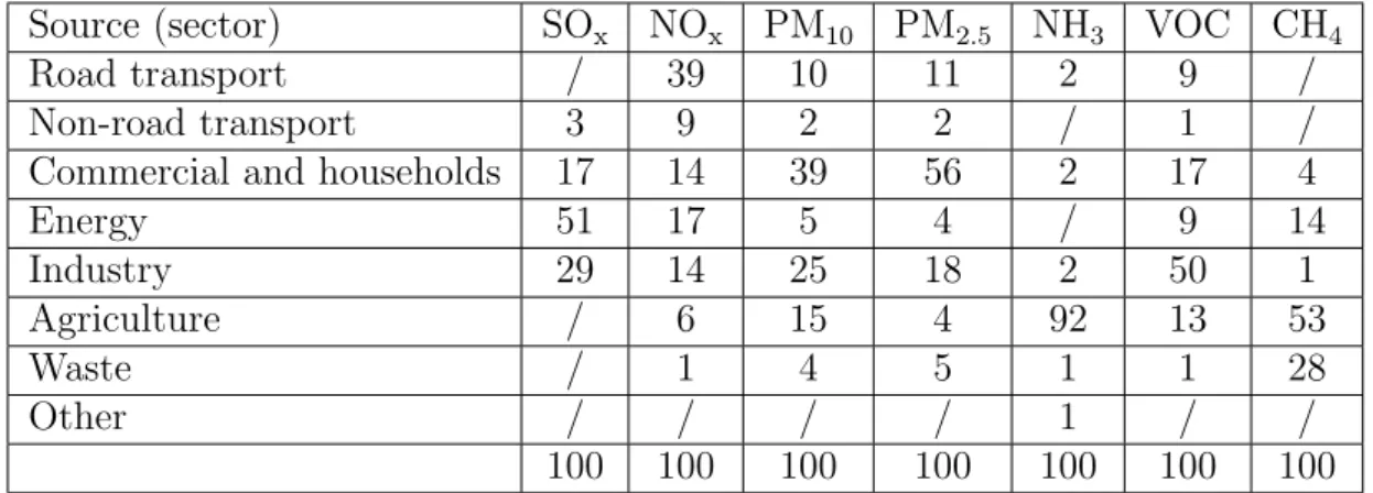
Considering only primary pollutants, it is possible to analyse the contributions of the various anthropogenic sources to air pollution: emission inventories, i.e. analyses that estimate the quantities of compounds emitted in the atmosphere by the various economic sectors, are common tools for reviewing and analysing these data. Table 1.1 summarizes the shares of contribution by each economic sector in the European Union member States in 2016, with respect to pollutants ([16]; only principal pollutants have been considered).

1.1.2

Geographical variability and concentration monitoring

The variety and the density of sources of pollutants in anthropized areas are responsible for generally significant emissions.

Nonetheless, pollutants concentration in a specific place is the result of transport and dispersion phenomena from the surrounding sources, as well as chemical reactions that produce secondary pollutants. Both processes are influenced by several meteorological variables and the morphology of the region (e.g. orography).

Source (sector) SOx NOx PM10 PM2.5 NH3 VOC CH4

Road transport / 39 10 11 2 9 /

Non-road transport 3 9 2 2 / 1 /

Commercial and households 17 14 39 56 2 17 4

Energy 51 17 5 4 / 9 14 Industry 29 14 25 18 2 50 1 Agriculture / 6 15 4 92 13 53 Waste / 1 4 5 1 1 28 Other / / / / 1 / / 100 100 100 100 100 100 100

Table 1.1: Share contribution of principal air pollutants per sector in EU-28 (2016).

1.2.

Indeed, depending on the location of the monitoring station, the concentration of a pollutant is given by:

• a regional background that can be detected anywhere in the considered area and is produced by the transport of pollutants in the atmosphere;

• a urban background that adds up to the previous one in urban contexts, where more sources are densely packed;

• the contribution from specific hotspots such as trafficked road and industries. So the regional background of a certain pollutant is related to a level of exposure of the population to that substance which is shared by all the inhabitants of the considered region, while the urban background is specific for residents in a certain urban area and hotspot levels can help assess the exposure of people who live by, work by or commute through particularly critical places.

Thus, sampling operations for analysing the concentration of pollutants are performed by a system of monitoring station placed at fixed locations in order to get a good rep-resentation of the considered area. In the EU framework, these locations are classified into:

• traffic: near trafficked roads, where concentration of various pollutants (NOx,

PM₁₀,. . . ) are generally high in specific periods of time during the day; • urban and suburban background: sites within a urban context;

Figure 1.2: Spatial distribution of a pollutant concentration (from [12]).

• rural background sites: far from the largest cities, in order to measure the regional background levels.

1.1.3

International policies

The huge number of effects and economic costs of air pollution has encouraged local, national and international authorities, along with other organizations, to take measures in order to limit the emission of pollutants.

The United Nations Environment Programme (UNEP) and the World Health Organi-zation (WHO) have guided the action at international level, calling for protection and promotion of people’s health and well-being, along with offering support to governments for undertaking monitoring and assessment of air quality issues, and taking measures to prevent and reduce air pollution.

At the European level, the framework of the EU’s air quality policy has been outlined in the 2018 Communication ”A Europe that protects: Clean air for all” [15]. It is composed

of three pillars:

• the ambient air quality standards defined in the Ambient Air Quality Directives (2004/107/EC [17] and 2008/50/EC [18]);

• the national emission reduction targets defined in the National Emissions Ceiling (NEC) Directive (2001/81/EC as replaced by Dir. 2016/2284/EU) with limits that have to be complied with starting from 2020 and 2030;

• the emissions standards for key sources of pollution, defined in a number of Di-rectives addressed to industries, power plants, vehicles, transport fuels and goods production.

At the national and local level, air quality plans to protect human health and environ-ment are requested by the Ambient Air Quality Directives, while National Air Pollution Control Programmes are expected by 2019 following the NEC Directive.

1.2

Particulate matter (PM)

The term particulate matter (PM) refers to the microscopic solid and liquid matter sus-pended in air; it has been defined by WHO [40] as “a complex mixture with components having diverse chemical and physical characteristics”, while the mixture composed of particulate and air is generally called aerosol.

Pollutants that belong to this category are generated through heterogeneous phase reac-tions, i.e. chemical reactions that involve compounds that are present in different phases in the atmosphere. Acid gases like sulfuric acid (H2SO4), nitric acid (HNO3) and

hy-drochloric acid (HCl) are often part of these reactions. An example of chemical reactions that lead to the formation of these compounds is given in the following formulas:

     SO_2(g)+ OH + O₂+ H₂O H₂SO_4(l)+ HO₂ 2NH3(g)+ H2SO4(l) (NH4)2SO4(s) NH_3(g)+ H₂SO_4(l) (NH₄)HSO_4(s) (1.1) ( NO_2(g)+ OH HNO_3(g) NH_3(g)+ HNO_3(g) NH₄NO_3(s) (1.2) NH3(g)+ HCl(g) NH4Cl(s) (1.3)

As can be seen, the interaction of this gaseous molecules with radicals and ammonia (NH3) produces solid salts that are incorporated by the aerosol.

The particles that make up particulate matter are generally classified by their aerody-namic diameter, a property that determines how particles are transported in the at-mosphere and deposited in the environment, and how they interacts with the human respiratory system (the diameter influences the likelihood of deposition in the different sites). Aerodynamic diameter is approximately linked to the source or the processes that generate particles; it can consequently be exploited in the sampling operation to separate the different classes of particles and identifying the most probable sources.

Following this criteria, PM particles can be classified in:

• coarse particles (PM10, or more correctly ”PM10- PM2.5”), i.e. whose aerodynamic

diameter is smaller than 10 µm and larger than 2.5 µm: these particles are gen-erally produced breaking up larger solid particles, and include resuspended dust (by roads, industrial activities, agricultural processes, uncovered soil, . . . ), pollen grains, bacterial fragments, sea-spray particles and ashes;

• fine particles (PM2.5), whose aerodynamic diameter is smaller than 2.5 µm: they are

formed from gases, where ultrafine particles are generated through the processes of nucleation, coagulation (combination of two or more nuclei) and condensation (of gas or vapour molecules on the surface of nuclei), that can produce fine particles up to 1 µm in terms of aerodynamical diameter; fine particles are also produced in combustion processes, where vaporized metals and organic compounds can con-dense: SO2, NOx, NH3 and VOCs are identified as PM2.5’s main precursors;

• ultrafine particles, whose aerodynamic diameter is smaller than 0.1 µm.

As said, the analysis of the chemical composition of PM allows to identify different sources, either natural or anthropogenic. Studies suggest that, in developed countries, more than 2/3 of PM2.5 can be attributed to anthropogenic sources.

Considering natural sources, the main contributors to PM concentration are wildfires and desert dust. It has been found [33] that their contributions to PM₁₀ and PM_2.5 in Europe are estimated in 4 ÷ 8 µg/m3 _{and 1 ÷ 2 µg/m}3 _{respectively.}

On the other side, the most important anthropogenic sources of PM are fossil fuel com-bustion (for energy production, heating and transport), biomass burning (in residential heating, agricultural burning and wildfires) and agricultural NH3 emissions, as seen in

the previous section. Part of these sources emit larger quantities of pollutants in winter: then this behaviour influences differently the concentrations of PM₁₀ depending on the season of the year.

It is worth noting that, along with the reduction of anthropogenic emissions expected at the EU level, natural ones are destined to increase their relative importance in the whole. Some works [28] have also predict that wildfires will increase due to climate change: in the future, their effect on PM concentration could then approach (even exceed in some cases) that of anthropogenic emissions.

1.2.1

Effects on human health

The main reason for considering PM a matter of concern is the negative effects it has on human health.

Epidemiological and clinical studies have connected PM exposure to a number of nega-tive health outcomes [40], from lung and respiratory system inflammation to increased risk for myocardial infarction, atherosclerosis, hospital admission and mortality in pa-tients with a variety of diseases (chronic obstructive pulmonary disease, cardiovascular diseases) and respiratory cancer.

Due to the heterogeneity of PM composition, the potential of particles to produce adverse health effects depends not only on the size, but also on the composition and consequently on the sources that produced the various parts of the mixture.

Thus, being each epidemiological study related to specific places and periods of time, measurements of the whole PM mass concentration allow to infer only approximately the presence of the various components of PM in the air. In order to understand the different effects of PM component on human health, specific sampling of each component is required.1

Studies regarding personal PM exposure, which is related to the overall average concen-tration a person is subjected to in a certain period of time, can’t take into account only outdoor PM concentration: having it been demonstrated that indoor PM levels can be significantly higher than outdoor concentrations at a certain time, a full characterization of the personal exposure is required in order to completely analyse the causal relationship between exposure itself and a range of diseases that could be observed.

Another factor affecting personal exposure is the variability of PM concentrations, also within the same city, as demonstrated by differences of daily values between roadside and urban background monitoring stations: people who live in a district can be exposed to a different outdoor concentration than those residing in another. Furthermore, living near busy streets generally means being exposed to higher concentrations.

Commuting is another important factor that affects personal exposure: PM concentra-tion inside a car can reach values that are 5 ÷ 10 times higher than those of a roadside monitoring station placed nearby.[40]

Personal exposure is also generally higher for children and people that exercise outdoor, due to the increased minute ventilation per unit mass with respect to an average person.

1_{It is worth mentioning that the improvement in sampling technologies has increasingly allowed to}

start routine and continuous measurements of single PM components and measurements of particle num-ber concentration (particularly useful for ultrafine particles), along with the continuous measurements of PM10and PM2.5mass concentration: these data can positively influence the depth of studies on the

It is necessary to take into consideration also the biopersistence that characterizes mainly insoluble particles (black carbon, in particular).

In fact, about one third of insoluble/biopersistent particles are retained in the lungs for long periods of time (even years).

Toxicological studies are trying to understand which characteristics of PM produce neg-ative consequences for people health.[40]

PM particles are inhaled and deposited throughout the respiratory system, and then deposited selectively depending on their size. The effects can be directly related with the respiratory system (inflammatory response, aggravation of existing diseases, weakening of defence mechanisms, e.g. against bacteria), worsening asthma and even allergies. Furthermore, these effects can induce secondary reactions in other systems, or particles can get through the respiratory tract and enter the body.

Toxicity arises from the interaction of PM particles with biological tissues: in particular, each component of PM interacts with different biological systems. A number of features of the particles (size fraction, mass concentration, number concentration, acidity, con-stituent chemicals, water solubility, . . . ) can favour those interactions and are currently under examination.

Critically, particle size is partially correlated with a number of features (e.g. chemi-cal composition), making it difficult to understand which are the actual effect-related features. The identification of particle-size-dependent effect independent of chemical composition (i.e. caused by the mere presence of PM in the affected tissue) can help in these kind of analysis. In the case of ultrafine particles, for example, the small size itself produces a more significant response by pulmonary tissues with respect to larger particles with the same chemical composition and mass concentration.2 _{On the other}

hand, particles can catalyse chemical reaction on their surfaces and also act as carrier of toxic chemical compounds, allowing them to reach the inner regions of the respiratory system.

1.2.2

Legal thresholds and guideline values for concentration

In the European Union, the reference values for PM10and PM2.5concentration have been

established by:

• the air quality standards for the protection of health, as defined in the Ambient Air Quality Directives ([17], [18]), that set legal thresholds which must be respected;

2_{Actually, studies have found that ultrafine particles can get translocated from the respiratory system}

to the brain, the nervous system and the liver, aside from being able to affect cellular organelles. The evaluation of the relation with brain tumour is currently under assessment [38].

• the WHO Air Quality Guidelines, updated in 2005 ([39], [40]). Table 1.2 and 1.3 summarize the reference values for both pollutants.

It must be noted that two additional targets for EU member States have been sets by EU Directives for PM2.5, based on the Average Exposure Indicator (AEI), i.e. the

3-year average of concentration values for a set of urban background stations selected on purpose by every national authority. These targets are:

• the Exposure Concentration Obligation, i.e. the target AEI value to be reached in 2015 (averaging 2013-2015 concentration values), set at 20 µg/m3_;

• the National Exposure Reduction Target (NERT), i.e. the percentage of reduction in AEI (comprised between 0% and 20%, with different values for each EU member State) to be met in 2020.

Reference value name Averaging period Value Max n. of exceedances

Daily limit value (EU) 1 day 50 µg/m3 35 days per year

Annual limit value (EU) Calendar year 40 µg/m3 _/

Daily AQG value (WHO) 1 day 50 µg/m3 3 days per year

Annual AQG value (WHO) Calendar year 20 µg/m3 _/

Table 1.2: Reference values for PM₁₀ concentration limits.

Reference value name Averaging period Value Max n. of exceedances

Annual limit value (EU) Calendar year 25 µg/m3 _/

Daily AQG value (WHO) 1 day 25 µg/m3 _{3 days per year}

Annual AQG value (WHO) Calendar year 10 µg/m3 _/

Table 1.3: Reference values for PM2.5 concentration limits.

1.2.3

Emission and concentration monitoring

Natural sources (like desert dust transport events and wildfires) can’t be controlled and usually contribute to background concentration, but also to high-concentration PM pol-lution events.3

As concerns anthropogenic sources, both primary PM and precursors emissions must be considered for assessing the contribution from the different sources.

In the European Union (see Figure 1.1), the periodic monitoring lead to observe that the emissions of secondary PM precursors (NO_x, SO_xand VOCs, with the important excep-tion of NH3) have been reduced more remarkably than primary PM emissions ([16]).

As said above, particulate matter concentration in the atmosphere is a critical subject of monitoring for multiple reasons, going from human health protection to assessment of air quality improvement measures. PM concentration is connected both to primary PM emissions and secondary PM produced by chemical reaction in atmosphere and to meteorological and geomorphological conditions that facilitate translocation, dispersion and deposition of pollutants far from their sources; secondary PM generation itself is linked to various environmental factors that influence the mentioned reactions.

The European Environment Agency periodically monitors the reference values for PM10

and PM_2.5concentration in 39 countries (28 member States and 11 other reporting coun-tries), assessing the compliance with EU legal thresholds.[16]

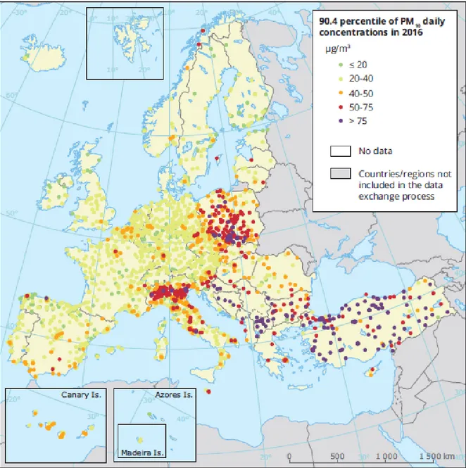
Figure 1.3 shows the results of 2016 monitoring on about 2900 stations for the EU daily limit value of 50 µg/m3_{: in particular, each point shows the 36}th _{highest daily mean}

concentration value in the year. Since the threshold can be exceeded for 35 days at maximum, a point in the map that go beyond that reference value actually corresponds to a non-complying site.

In 2016 19% of the reporting stations exceeded the limit value. Notably, 97% of these stations where either urban or suburban sites.

The annual mean concentration values for PM10 in 2016 with respect to the EU limit

value of 40 µg/m3 _{are reported in Figure 1.4.}

In this case, only 6% of the considered station reported a value above the threshold. It is also interesting to mention that 48% of the considered stations exceeded the WHO guideline values for the mean annual concentration (20 µg/m3_{). As can be seen from the}

3_{Specific environmental conditions can lead to the so-called PM pollution episodes [16], defined as}

large-scale events of widespread high values of concentration for PM10or PM2.5. Such events generally

happen in autumn, winter or spring, when favourable meteorological conditions combine with large anthropogenic emissions (mainly in the agricultural or residential sector) and the eventual addition of contribution from natural sources (e.g. dust transport). In these situations, the level of PM concentra-tion can exceed the reference values (guideline values or even legal thresholds) for several days.

Figure 1.3: PM₁₀daily mean concentrations in Europe in 2016 - 36th _{highest value}

map, only four countries (Estonia, Iceland, Ireland and Switzerland) have all the stations annual mean below this value.

The last two maps show large areas where PM10concentration values are generally high:

the Po valley, eastern Europe, the Balkans and Turkey. Apart from the first region, the others show exceeding values both in the daily and the annual limit values.

Figure 1.5 shows the annual mean of PM_2.5 concentration values for 1327 monitoring stations in 2016, with respect to the EU limit value of 25 µg/m3_.

In this case, values above concentration threshold were reported from 5% of the moni-toring station, mainly (97%) in urban areas.

Concerning WHO annual guideline value (10 µg/m3_{), it was exceeded at 68% of the}

stations; five countries (Estonia, Finland, Hungary, Norway and Switzerland) reported only values below the guideline.

1.3

Context overview: Emilia-Romagna

Various characteristics of Emilia-Romagna, the Italian administrative region whose area is the research field of this work, make it a place where pollutant concentrations (PM, O₃ and NO₂ in particular) regularly exceed the EU legal thresholds.

In this region, the Regional Agency for Prevention, Environment and Energy (ARPAE, Agenzia Regionale per la Protezione dell’Ambiente e l’Energia) is the public agency responsible for monitoring air quality, drafting emisson inventories and assessing the impact of measures addressed to air pollution issues in the region.

1.3.1

Geographical and meteorological elements

Emilia-Romagna is located in the Po-Adriatic basin: half of the region (the north-north-east part) corresponds to a flat strip on the southern side of the Po river, while the other half is characterized by a portion of the Apennine chain of mountains. The whole Po-Adriatic basin is sorrounded by the Apennines (southern edge) and the Alps (western and northern edges), while the Adriatic sea closes the area on the east side.

Although westerly winds are prevalent at these latitudes, the enclosing orography of the basin determines unfavourable conditions for the dispersion of air: in fact, calms charaterizes the wind regime of the region, as air circulation between northern Italy and the rest of the continental Europe is hindered by mountains, and dispersion processes in absence of significant wind require days in order to remove pollutants from the air. In the low Po valley wind speed does not exceed 2.5 m/s in general (4 m/s can be reached on the coast) and the mixing of air is due primarily to the thermal component of the wind, which depends on the solar radiation: as radiation increases during summer months, this leads to a reduction in concentrations for various pollutants (including PM and NO2).

Therefore a useful meteorological parameter is the mixing height, which describes the vertical depth (above surface) which is available for air mixing processes such as con-vection. As it will be seen, its value is particularly low during winter months since it is correlated with the presence of the thermal component of the wind.

In the same period it is common to see temperature inversion: this term refers to the situation in which a warmer air mass is found above a colder one that is immediately near the surface. In this condition, convection is hindered so that air stagnates and pollution tends to build up, leading to very high concentrations that are quite homogeneous in the whole area.

On the other hand, during summer months photochemical pollution (that involves O3)

is enhanced by solar radiation and higher temperature: for this reason a variety of secondary pollutants show higher concentrations during this period. As mentioned above, the stronger thermal component of the wind during summer allows a more effective

mixing in the atmosphere, a condition that produces an approximately homogeneous distribution of these pollutants in the basin.

1.3.2

Anthropic pression and emission sources

The Po-Adriatic basin is home to over 23 million people (nearly 40% of the Italian population). This macroregion contributes to over the 50% of the national GDP.

In this context, Emilia-Romagna is characterized by a high population density in its flat part (198 inhabitants/km2) and a total land consumption of about 10% of its total surface area.

Cities and industrial areas are concentrated along the main communication routes. The rest of the flatland is occupied by intensive agriculture and animal farming.

The urban polycentrism that characterizes the area is the cause of the great demand of mobility, that in turn produces huge emissions in the transport sector; this adds to transit traffic, due to the central position of the region with respect to the main national routes.

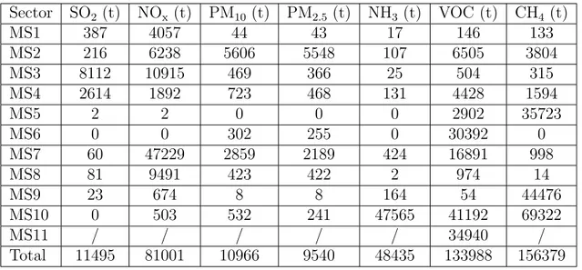
The strong anthropization of the region, with the concentration of economic activities (industrial, agricultural and farming sector), vast residential areas and the aforemen-tioned high levels of traffic, is responsible for the important emissions of air pollutants. As said, ARPAE is responsible for drafting emission inventories for the region. In Table 1.4 the contributions to the emission of pollutants from the different economic sectors for the year 2015 are reported, as provided in the last report available [3].

Sector SO₂ (t) NO_x (t) PM₁₀(t) PM_2.5 (t) NH₃ (t) VOC (t) CH₄ (t) MS1 387 4057 44 43 17 146 133 MS2 216 6238 5606 5548 107 6505 3804 MS3 8112 10915 469 366 25 504 315 MS4 2614 1892 723 468 131 4428 1594 MS5 2 2 0 0 0 2902 35723 MS6 0 0 302 255 0 30392 0 MS7 60 47229 2859 2189 424 16891 998 MS8 81 9491 423 422 2 974 14 MS9 23 674 8 8 164 54 44476 MS10 0 503 532 241 47565 41192 69322 MS11 / / / / / 34940 / Total 11495 81001 10966 9540 48435 133988 156379

Table 1.4: Contribution of principal air pollutants per sector in EU-28 (2016). Sectors are classified following the SNAP (Selected Nomenclature for sources of Air

Pollution) coding, required by the CORINAIR metodology; the economic sectors for each class are specified in Table 1.5.

Class Economic sectors Class Economic sectors

MS1 Energy production and fuel reprocessing MS7 Road transport

MS2 Non-industrial burning MS8 Other mobile sources and machineries

MS3 Industrial burning MS9 Waste processing and disposal

MS4 Production processes MS10 Agriculture

MS5 Fuel extraction and distribution MS11 Other sources and absorptions

MS6 Use of solvents

Table 1.5: Sectors included in SNAP coding.

1.3.3

Air quality and meteorology

The load of anthropogenic primary emissions in the basin, together with meteorological factors that determine air stagnation, leads to high concentrations of various pollutants that facilitate the formation of secondary pollutants. Significant levels of concentration tend to persist at ground level until major meteorological events (winds, rains) of suffi-cient strenght allow the removal of pollutants through transport or deposition.

As already said, emissions are only the starting element in the process of air pollution, while meteorological factors are the main responsibles for the processes of dispersion, translocation and catalysis of chemical reactions that produce secondary pollutants. Thus a statistical assessment of the influence of meteorological factors on the concentra-tion of pollutants is of particular interest in order to evaluate the condiconcentra-tions that favour the building up and the dispersion of pollutants. Such analysis is the particular focus of the present work.

1.3.4

Regional concentration monitoring

In order to measure regularly pollutants concentration, a monitoring network has been es-tablished by ARPAE within the regional borders: it is composed of 47 monitoring station equipped with automatic analysers for different compounds (nitrous oxides, particulate matter, ozone,. . . ; each station can have a different combination of these instruments). Following the national legislation (dlgs. 155/2010, art. 3), the region has been divided into four zones: Agglomerato (that includes the regional capital and its neighbouring towns), Appennino, Pianura ovest and Pianura est.

Similarly to the geographical classification of sites given in a previous section, ARPAE monitoring stations are classified into 4 categories according to their location. Each category is characterized by a specific combination of measure instruments, as follows:

• 12 Traffico Urbano (TU; traffic) stations, equipped with PM10 and NO2 analysers

(sometimes also with CO and C6H6 (benzene) analysers);

• 21 Fondo Urbano (FU) and Fondo Suburbano (FS) (urban background) stations, equipped with PM10, PM2.5, O3and NO2analysers; some FU stations are also used

to collect samples of PM in order to periodically determine some metals (Pb, As, Ni, Cd) concentrations;

• 14 Fondo Rurale (FR; regional background) stations, equipped with PM10, PM2.5,

O3 and NO2 analysers;

Figure 1.6 shows the locations of the monitoring stations on the regional area; the num-ber of station per category and zone is summarized in Table 1.6.

Zone TU FU FS FR Total per zone

Agglomerato 2 1 1 0 4

Appennino 0 0 0 5 5

Pianura ovest 5 5 4 4 18

Pianura est 5 6 4 5 20

Total per class 12 12 9 14 47

Table 1.6: Number of monitoring station per zone and category.

The results of monitoring on air pollutants reported by ARPAE for 2017 are obtained applying a geographical model based on data recorded by urban and rural background stations.[1]

As can be understood by Figure 1.7, in that year the plain part of the region has been affected by several exceedences of EU daily limit value of 50 µg/m3 for PM10: in

par-ticular, the northern area that encloses the cities of Piacenza, Parma, Reggio Emilia, Modena and Ferrara has illegally passed the threshold of 35 daily exceedances in the year.

The map does not allow to figure out if the WHO guideline objective for exceedances (3 days per year at maximum) of the same daily mean concentration value was met in any part of the region.

Figure 1.7: PM₁₀ daily mean concentrations in Emilia-Romagna in 2017 - Number of exceedances of the limit value (estimate) (from [1]).

Talking about the annual mean concentration of PM10, the map in Figure 1.8 shows that

the EU limit value of 40 µg/m3 _{has not been exceeded in any part of the region.}

On the other hand, it must be noticed that the WHO guideline for the same reference value (20 µg/m3) was exceeded in the whole plain part of the region.

Figure 1.8: PM₁₀ annual mean concentrations in Emilia-Romagna in 2017 (estimate) (from [1]).

The annual mean concentration estimate for PM2.5 is shown in Figure 1.9. Exceedances

of the EU limit value (25 µg/m3_{) are confined to small rural areas in the northern part}

of the region.

At the same time, the WHO guideline value (10 µg/m3) is exceeded in most of the regional area, including in the Apennine valleys.

1.4

Models for PM

prediction

The final aim of this work is to develop a statistical model based on machine learning able to predict PM10 concentration levels by exploiting the relationship between the

pollutant’s concentration and meteorological conditions observed in the capital cities of the provinces of Emilia-Romagna.

A similar classification task has been previously performed for the regional area, as outlined in the 2018 report on regional air quality published by ARPAE.[1] In that

Figure 1.9: PM2.5 annual mean concentrations in Emilia-Romagna in 2017 (estimate)

(from [1]).

report two syntetic indicators for the evaluation of the meteorological condition that can favour the building up of pollutants (the number of favourable days for PM₁₀ build-up and the number of favourable days for O3build-up) are presented: these indexes represent

the days in which meteorological conditions are “good” for the generation and build-up of the pollutant, i.e. the days characterized by a high probability that legal threshold would be exceeded.

The meteorological parameter values that define the favourable conditions have been obtained [4] using classification tree technique on a dataset of significant meteorological variables corresponding to one year of observations in Bologna, recorded in the Giardini Margherita monitoring station. The model has been used in order to make predictions for the whole regional area, despite being trained on local data.

The analysis performed by ARPAE on the meteorological data for years 2008-2017 has lead to the results shown in Figure 1.10, that describes the percentage of days (with respect to the considered seasons) in which the model predicts that the concentration of the pollutant will exceed the legal threshold.

As the task was similar to the one of the present work (in particular for the geographical area that was considered), it must be reported that no information has been obtained from the author of [4] apart from those aforementioned: in particular, no precise

tempo-Figure 1.10: Share of favourable days for PM10 (during autumn and winter; on the left)

and O₃ (during spring and summer; on the right) build-up in 2008-2017 (from [1]).

ral information on the considered set of data, nor the dataset itself, nor the reasons for which a classification tree was chosen as model have been made available.

Since the lack of information made it impossible to use the results obtained by the clas-sification tree applied on data from Bologna as a benchmark, while on the other hand literature provides a large number of works in which quantitative predictions have been performed starting from similars sets of meteorological data, a completely independent analysis has been performed starting from a newly assembled dataset on the same kind of data, geographically widened in order to comprehend all the provincial capital cities of Emilia-Romagna, so to achieve a quantitative result similar to the one obtained in [4] for each city separately.

In the next paragraphs, an overview of past works is made. The main focus of the research is that of stastical models based on machine learning which have been applied to tasks similar to the one of interest fot the present work.[35]

As different kinds of models can be applied for the task of predicting a pollutant’s concentration [5], here only statistical methods have been considered. Other kinds of models, such as numerical ones, have not. There are in fact important differences between these two categories: numerical models are based on a simulation of the concentration of pollutants on spatial and temporal scales, based on the chemical and physical processes that take place in the atmosphere, where the geography of the considered area, the atmospheric behaviour in a layer of defined height, the position and the characteristics of the sources of emissions and other inputs of the model must be characterized on a defined temporal scale. Characterizations of this kind can be performed using suitable

simulation models that starts from information given on a discrete spatial and temporal scale and determines numerically the most likely behaviour for each considered variable. These models can be characterised by a significant precision both in the spatial and temporal scales; on the other hand, the volume of data and the computational costs that are necessary in order to run them are relevant. On the other hand, a different kind of results can be obtained by using statistical models: these does not take into account the physical and chemical processed given a certain geospatial region of interest, but evaluate the behaviour of a number of input variables in a statistical way in order to predict output descriptors that are related to the considered predictors. As the geographical range of those models can be reduced to a point-level prediction, the quantity of necessary data is reduced and in general they are more easily available thanks to the presence of various open databases.

1.4.1

Previous works on PM

forecasting

A study performed on a 1999-2001 dataset of 5 meteorological variables collected in the metropolitan area of greater Athens [9] presents a comparison between multilinear regression techniques and feed-forward multilayer perceptrons. The best performer, a multilayer perceptron trained only on meteorological data, was characterized respec-tively by R2 _{= 0.47 (0.03) and RM SE = 21.19 (0.95) µg/m}3_{. Adding the previous-day}

PM10 concentration values to the set of predictors improved the performance of that

model, leading to R2 _{= 0.65 (0.03) and RM SE = 16.94 (0.76) µg/m}3_.

Similar works have also involved PM10 hourly concentration prediction: in [25]

multilin-ear regressions and multilayer perceptrons were trained on data taken from four different locations in Greater Athens; the best RMSE (12.16 (0.67) µg/m3_{) was obtained with a}

multilayer perceptron coupled with a genetic algorithm for variable selection.

Another work on PM10 hourly concentration prediction was performed on data (both

meteorological and descriptive, as ”day of the week”) collected in 2005 in Phoenix, Arizona [22]: a comparison between a deterministic model (Community Air Quality Modelling System, or CMAQ ) and a statistical one (3-layer neural network) was made, resulting in RMSE values of 25 ÷ 40 µg/m3 with the statistical model performing better.

1.4.2

Previous works on other pollutants’ forecasting

In order to get a wider knowledge of previous efforts in the statistical modelling field applied to the task of pollutant concentration prediction on a meteorological basis, other works have been considered.

A study on 8 USA cities [11] comparing the performance of multilinear regressions and neural networks in predicting O₃ daily maximum 1-hour concentrations starting from a dataset of four meteorological variables showed that neural network generally outper-forms multilinear regressions. The best result for both algorithms was obtained consid-ering also the previous-day value of O₃ concentration: in the best case (neural network) the regression reached R2 _{= 0.69 (0.04) and RM SE = 9.24 (0.54).}

In Canada, a classification tree analysis on maximum surface O₃ daily observation has been performed on a 1985-92 dataset concerning the areas of Vancouver and the lower Fraser River valley [6]: the study, which has been considered useful for the wide range (57) of variables chosen as predictors, describes a categorical approach in considering the response variable (i.e. predictions and measured values were classified with respect to 2 thresholds and matching between classes has been evaluated).

A comparison between multilinear regression, ARIMA model and neural networks was performed on a 1993-1994 dataset containing temperature- and wind-related variables, along with emissions of a number of gaseous compounds, in order to evaluate the best result in predicting hourly daily maximum ozone level O3in Dallas, Texas [42]. The best

result was achieved by the neural network, with a MAD of 6.4ppb ≈ 12.8 µg/m3.

An attempt to model hourly concentrations of NOxand NO2 in Central London starting

from a dataset of 6 meteorological variables, which was supplemented with sinusoidal indexes accounting for the hour of the day or with the previous-hour concentration of either NOx or NO2, was made using multilayer perceptrons [23]. The best model, which

used the lagged concentration for NOxprediction, reached a best R2 value of 0.92 (0.02)

corresponding to RM SE = 33.8 (2.3).

Furthermore, a comparative study in 5 UK cities [24] aimed to analyse the performances of multilinear regression, regression trees and multilayer perceptrons on a dataset of 7 meteorological variables from the period 1993-1997 in order to predict hourly O₃ con-centrations; seasonal sinusoidal indexes representing the day of the year and the time of the day were also added in order to account for periodical variation of emissions of pre-cursors. The best test R2 _{value was 0.68 (0.01), corresponding to RM SE = 6.60 (0.13).}

The Greater Athens Area hosted further analysis. One [43] was performed on 1987-1990 meteorological data (3 variables), along with previous-day maximum hour concentration of NOx and day of the week index, which were used to predict both the the increase

or decrease of the concentration of the same pollutant and a numerical forecast of that concentration. In the second task the best achieved test RMSEs were of 45µg/m3 _(in

case of increasing concentration) and 35µg/m3 _{(in case of decreasing concentration).}

Again in Athens, a dataset collected in the summer months of 1987-1993 has been used to evaluate regression models for the prediction of the daily maximum of O₃ hourly

concentrations [7]. The works involved both meteorological variables, previous-day O3

hourly maximum and the same-day concentrations of precursor gases NO₂and CO, which were feeded into multiple linear regression and ARIMA model. The best performed showed a RMSE of 47.99 µg/m3.

Another work [10] focused again on maximum hourly concentration of O₃, starting from summer data collected in Athens during 1992-1999, in order to compare multilinear regressions and neural networks. A set of 8 meteorological variables was considered, while O₃ measures were taken from 4 nearby monitoring stations. In this case the best reported R2 _{was 0.59 (0.01), corresponding to a RMSE of 21.7 (0.7) µg/m}3_{, obtained}

using a neural network.

In the same area, an analysis concerning O₃ and NO₂ daily concentration levels em-ployed feed-forward neural networks that were trained using four meteorological vari-ables, previous-day concentration and an index representing the day of the week [32]. Best model R2 _{of 0.802 for O}

3 and 0.690 for NO2,corresponding to RMSE values of

27.4 µg/m3 _{and 39.3 µg/m}3 _{respectively.}

In Beijing, data of three meteorological variables and UV radiation taken during a single summer period were used as predictors for ozone concentration. The results were pro-duced by neural networks of different kind [21]: the best R2 of 0.76 (0.01) (corresponding to a RMSE of 36.56 (5.15) µg/m3_{) was obtained from a neural network trained with}

ge-netic algorithm coupled with a SVM classifier.

A work on Besiktas district in Istanbul [30] was focused on forecasting SO₂, CO and PM10 levels using neural networks feeded on the basis of spatial criteria: this was made

possible by the presence of a network of monitoring stations located in neighboring districts. A non-geographical model (which used only data from Besiktas) with 9 me-teorological variables and the same-day level of the considered pollutant was compared with 1-, 2- and 3-neighborhood-trained models in which the set of input variables was expanded on a geographical basis; in the last case, the same-day level of pollutant was feeded to the model as a weighted sum of the concentration levels measured in the con-sidered neighboring districts. The results were reported as error rates based on a error grid: the comparison showed that the 3-neighboring-districts model gave the best results. A comparison between standard multilinear regression on 14 meteorological variables measured in New Delhi in 2000-2006 and the same model feeded with principal compo-nents of the dataset (the overall algorithm is called “principal component regression”) was made in order to predict the values of the Indian Air Quality Index [29] (a con-tinuous numerical value in the interval 0 ÷ 500, related to the presence of pollutants in the air). The results of the analysis, performed separately for the four seasons, shown a generally better beahviour of the coupled model, with the best R2 of 0.5767 (RMSE of 30.90) achieved for the winter season.

1.4.3

Some remarks

Being aware of the results presented in the described works, the aim of the present one is to develop a similar quantitative approach starting from the classification model proposed in [4] and widening the geographical range of the analysis to the capitals of the provinces of Emilia-Romagna.

As seen in the previous paragraphs, a number of machine learning methods have been used in tasks similar to the one that is presented in this work. In particular, city-level approach is common since the urban areas are generally more affected by air pollution than rural ones. Noticeably, none of the articles that have been found concerns the geo-graphical region that is analysed in the present work.

The prediction quality significantly varies depending on the work: this can be related to the representativeness of the meteorological quantities in describing the conditions in which the data from PM10 monitoring stations have been collected, the kind of source

of pollution that are present in the area and other context-related issues that can affect the modelling results. Obviously also the kind of models that have been applied strongly influence the performance.

It must also be noticed that, in a number of cases, the chosen task concerns forecasting the concentration of pollutants for the day following the one in which the measurements have been performed. This purpose can be more interesting from a administrative point of view, since it can provide information in advance to decision-makers so that they can enforce restrictions and other measures in order to tackle a potential critical situa-tion. However, in accordance with the previously described classification model built by ARPAE, it has been chosen not to consider previous-day values of meterological vari-ables for the regression models that have been trained and to limit the predictors to the same-day quantities.

So, concerning the present work, the assessment has been made on two kind of regression models: standard and regularized linear regression models and regression tree-based models. The first have been chosen since they are widely used as a basis point for a large number of works in the cited literature, while the second ones are the counterparts of the classification tree model whose results have been used by ARPAE in [1] to assess the number of days with favourable meteorological conditions for the build-up process of pollutants.

The previous literature review is also useful, apart from providing a framework of models and sets of meteorological and non-meteorological variables that have been used for sim-ilar modelling tasks, to give suggestions for further developments of the present analysis (see Chapter 4).

Chapter 2

Materials and methods

In this chapter a description of the data and the models that have been used in this work is given. Starting from an exploratory analysis of the dataset, the chapter contin-ues with a presentation of the algorithms that have been used to address the problem of missing data and to perform modelling tasks: as already explained, the aim is to find the regression model that gives the best prediction of PM10concentration values starting

from the values of the meteorological variables measured in the same day.

In section 2.1 the dataset of the considered variables is presented and analysed using exploratory data analysis (EDA) techiniques, with a focus on the relationship between each variable and PM₁₀ concentration. The aim is to provide a first overview on the meteorological variables, their trends and distributions in the considered period of time. In section 2.2 the problem of missing data is addressed and the methods that have been applied on the considered dataset is presented. Subsequently the regression models are presented: in section 2.3 the considered linear models for data regression and prediction are described; in section 2.4 the applied regression tree methods are explained. Then, in section 2.5, the procedure of cross-validation which has been used to assess the perfor-mance of the chosen regression models is outlined.

Finally, the implementation of the models and the assessment procedures using the R-based software RStudio are described in section 2.6.

2.1

Data overview and exploratory analysis

In this section a general overview of the considered set of data and basic statistical analysis techniques that have been used in order to make an exploratory data analy-sis are presented. Each variable is described and analysed separately, highlighting its relationship with PM₁₀concentrations.

Concerning the dataset in general, a group of daily-measured meteorological variables has been included in it along with the values of PM₁₀ daily mean concentrations. Meteorological variables have been downloaded by the applet Dext3r1_{, that allows the}

user to define the set of variables , the time window and the location of interest. PM10

daily mean concentrations are available on the ARPAE website, in the thematic section “Aria”2_{, in which a page for each monitoring station is present.}

Each considered variable corresponds to daily-measured or calculated values in the period of time between the 1st of October, 2012 and the 31st of March, 2018. The measuring processes have taken place in all the provincial capital cities of Emilia-Romagna: Pia-cenza, Parma, Reggio Emilia, Modena, Bologna, Ferrara, Ravenna, Forl`ı, Cesena and Rimini. The overall number of considered days is 2008.

PM10 concentrations have been measured in the monitoring stations classified as Fondo

Urbano, while the meteorological variables have been measured by urban meteorological stations that are part of ARPAE meteorological network3_.

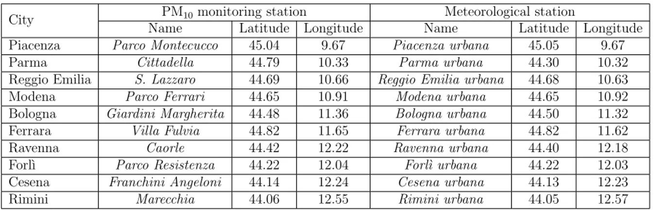
In Table 2.1 the lists of the considered monitoring stations for PM10 and of the

meteo-rological stations are presented.

City PM10monitoring station Meteorological station

Name Latitude Longitude Name Latitude Longitude Piacenza Parco Montecucco 45.04 9.67 Piacenza urbana 45.05 9.67

Parma Cittadella 44.79 10.33 Parma urbana 44.30 10.32

Reggio Emilia S. Lazzaro 44.69 10.66 Reggio Emilia urbana 44.68 10.63 Modena Parco Ferrari 44.65 10.91 Modena urbana 44.65 10.92 Bologna Giardini Margherita 44.48 11.36 Bologna urbana 44.50 11.32 Ferrara Villa Fulvia 44.82 11.65 Ferrara urbana 44.82 11.62

Ravenna Caorle 44.42 12.22 Ravenna urbana 44.40 12.18

Forl`ı Parco Resistenza 44.22 12.04 Forl`ı urbana 44.22 12.03 Cesena Franchini Angeloni 44.14 12.24 Cesena urbana 44.13 12.23

Rimini Marecchia 44.06 12.55 Rimini urbana 44.05 12.57

Table 2.1: Position of PM10 monitoring stations and meteorological stations in which

data has been measured.

The resulting dataset contains daily-calculated values for the variables summarized in Table 2.2. The properties of each variable are described in the following sections. The choice of the variables has been performed both by asking experts’ opinion and by reviewing literature4 (see “References” in Table 2.2).

As it is not unusual in the case of automated measuring devices, some missing values are present in the set. In Table 2.3 the absolute number of missing values by variable

1

Available at https://simc.arpae.it/dext3r/

2

Available at https://www.arpae.it/dettaglio_generale.asp?id=2921&idlivello=1637