AN ALTERNATIVE HYPER-POISSON DISTRIBUTION C. Satheesh Kumar, B. Unnikrishnan Nair
1. INTRODUCTION
Bardwell and Crow (1964) introduced a two parameter family of discrete dis-tributions namely the hyper-Poisson distribution through the following probabil-ity generating function (p.g.f.).
( ) (1; ; ) (1; ; ) G t t , (1) in which , 0 and 0 1 ( ; ; ) 1 ( ) k [( ) ! ] k k k a b z a z b k
is the confluent hypergeometric series (also called the Kummer M function), in
which ( )a is the rising factorial: k
( )a k a a( 1) ... (a k 1) (a k ) ( ) a ,
for 1, 2,...k and ( )a . For details on confluent hypergeometric series see 0 1
Mathai and Haubold (2008) or Abramowitz and Stegun (1965, chapter 13). When 1
, the hyper-Poisson distribution reduces to the Poisson distribution and
when is a positive integer, the distribution reduces to the displaced Poisson
distribution of Staff (1964). Bardwell and Crow (1964) termed the distribution as
sub-Poisson when and super–Poisson when 1 . The hyper-Poisson dis-1
tribution is also a member of the Kemp family of distributions studied by Kumar (2009). Various methods of estimation of the parameters of the distribution were discussed in Bardwell and Crow (1964) and Crow and Bardwell (1965). Some queuing theory associated with hyper-Poisson arrivals has been developed by Nisida (1962). The estimation of the parameters of the hyper-Poisson distribution using negative moments were attempted by Roohi and Ahmad (2003a). Roohi and Ahmad (2003a) derived expressions for ascending factorial moments of the
hyper-Poisson distribution and obtained certain recurrence relations for its nega-tive moments and ascending factorial moments. Kemp (2002) considered a q-analogue of the distribution and Ahmad (2007) introduced the Conway-Maxwell hyper-Poisson distribution. Kumar and Nair (2011, 2012) developed extended versions of the hyper-Poisson distribution and discussed some of their applica-tions.
In this paper, we consider an alternative form of hyper-Poisson distribution which we named as “the alternative hyper-Poisson distribution (AHP distribu-tion)” and study its important properties. In section 2 we give the definition of AHP distribution and derive its p.g.f., expression for factorial moments, raw moments, mean, variance, and recursion formulae for its probabilities, raw mo-ments and factorial momo-ments. Further the estimation of the parameters of AHP distribution by method of factorial moments, method of mixed moments and method of maximum likelihood are discussed in section 3 and illustrated using real life data sets.
We need the following series representations in the sequel.
0 0 0 0
( , )
x( ,
)
x r x rA r x
A r x r
(2) 0 0 0( , )
n( , )
r n r n rB r n
B r n
(3)2. THE AHP DISTRIBUTION
In this section we present the definition of the AHP distribution and obtain some of its important properties.
Definition 2.1. A non-negative integer valued random variable X is said to follow the alternative hyper-Poisson distribution (or in short the AHP distribution) if its
probability mass function (p.m.f.) has the following form, in which , 0 0
and x 0,1, 2,... ( ) [ ] f x P X x (1 ; ; ) ( ) x x x x (4)
Clearly, when the AHP distribution reduces to the Poisson distribution. 1
An important characteristic of the AHP distribution is that it is under-dispersed
when and over-dispersed when 1 , in the light of Remark 2.1. Now we 1
Result 2.1. The p.g.f ( )G t of the AHP distribution with p.m.f. (4) is the following.
( ) [1; ; ( 1)]
G t t (5)
Proof. By definition, the p.g.f. of the AHP distribution with p.m.f. (4) is
0
( )
( )
x xG t
f x t
0 (1 ; ; ) ( ) x x x x x x t
(6)On expanding the confluent hypergeometric series in (6), we get
0 0 (1 ) ( ) ( ) ( ) ( ) ! x r x r x r x r x t G t x r
0 0( )
(
)
(
)!
!
! ( )
x r x r x rt
x r
r
x
, (7) since ( ) ( x x)r ( ) x r and (1x)r ( !)x 1 (x r )!.Now applying (2) in (7) to obtain
0 0 ( ) ( ) ! ( ) ! ( )! ( ) x r r x x r x t x G t r x r
0 1 [ ( 1)] ( ) x x x t
, (8)in the light of binomial expansion of [ ( t 1)]x. Since (1) !
x x from (8) we have 0 (1) [ ( 1)] ( ) ( ) ! x x x x t G t x
, which is (5).Result 2.2. An expression for factorial moments [ ]r of the AHP distribution is
[ ] ! ( ) r r r r (9)
Proof. The factorial moment generating function ( )F t of the AHP distribution
with p.g.f. (5) is
( ) (1 )
F t G t
(1; ; t).
On expanding (1; ; t) and equating the coefficients of ( !)r 1tr, we get (9).
Result 2.3. Mean and variance of AHP distribution are
Mean = and Variance = 1 ( 1) ( 1) .
Remark 2.1. From Result (2.3) it is obvious that the AHP distribution is
under-dispersed (that is, mean greater than variance) when and over dispersed 1
when 1
Result 2.4. An expression for raw moments n of the AHP distribution is the
fol-lowing, for n . 0 0
!
( , )
( )
r n n r rr
S n r
, (10)where ( , )S n r is the Stirling numbers of the second kind. For details see,
(Riordan, 1968).
Proof. The characteristic function ( ) t of the AHP distribution with p.g.f. (5) is
0
( )
( )
!
n n nit
t
n
(11) G e( )it [1; ; (eit 1)]On expanding the confluent hypergeometric function and using the fact (1)r , r!
we get 0 [ ( 1)] ( ) ( ) it r r r e t
0( )
!
( , )
( )
!
n r r n r rit
r
S n r
n
, (12)since by the equation (1.57) of (Johnson et.al., 2005). By applying (3) in (12) we obtain 0 0
( )
!
( )
( , )
( )
!
n r n n r rit
r
t
S n r
n
(13)On equating the coefficient of ( !) ( )n 1 it n on right hand side expressions of (11)
and (13), we get (10).
Define the following shorter notations, which we need in the sequel. (1, ) and (1 , ) j j j , for 1, 2,... .j
Result 2.5. The following is a simple recursion formula for probabilities
( , ) ( )
x
f f x of the AHP distribution with p.g.f. (5), for x 0.
1( , ) ( 1 , ) ( 1) x x f f x (14)
Proof. From (4) we have ( ) [1; ; ( 1)] G t t 0 ( , ) x x x f t
. (15)On differentiating (15) with respect to t , we obtain the following.
1 0 ( 1) x ( , ) x [2; 1; ( 1)] x x f t t
. (16)Also, from (15) we have
0 [2; 1; ( 1] ( 1, ) x x x t f t
(17)Relations (16) and (17) together lead to the following.
1 0 0 ( 1) ( , ) x ( 1, ) x x x x x x f t f t
. (18)on equating the coefficients of tx on both sides of (18) we get (14). □
Result 2.6. The following is a recursion formula for raw moments ( ) r of r
the AHP distribution, for r 0.
1 0 ( ) r ( 1) r r k k r k
(19)Proof. On differentiating (11) with respect to t , we get the following.
1 1 ( ) [2; 1; ( 1)] ( ) ( 1)! r it it r r it e e r
(20) From (11) we have 1 ( ) [2; 1; ( 1)] ( 1) ! r it r r it e r
. (21)1 0 0 ( ) ( ) ( ) ( 1) ! ! r r it r r r r it it e r r
0 0 ( ) ( ) ( 1) ! ! k r r r k it it k r
0 0 ( ) ( 1) !( )! r r r k r k it k r k
, (22)in the light of (2). Now, on equating the coefficients of
( !) ( )
r
1it
r on both sidesof (22) we get (19). □
Result 2.7. The following is a simple recursion formula for factorial moments [ ]r ( ) [ ]r
of the AHP distribution, for r 1, in which
[0]( ) 1 . [r 1]( ) [ ]r ( 1) , (23)
Proof. The factorial moment generating function ( )F t of the AHP distribution with p.g.f. given in (5) has the following series representation.
( ) (1 ) F t G t (1; ; t) [ ] 0 ( ) ! r r r t r
(24)On differentiating (24) with respect to t to get 1 [ ] 1 (2; 1; ) ( ) ( 1)! r r r t t r
(25)By using (24) we get the following from (25).
[ 1] [ ] 0 0 ( ) ( 1) ! ! r r r r r r t t r r
(26)3. ESTIMATION
Here we consider the estimation of the parameters and of the AHP
dis-tribution by method of factorial moments, method of mixed moments and the method of maximum likelihood.
3.1 Method of factorial moments
In method of factorial moments, the first two factorial moments [1], of [ 2]
the AHP distribution are equated to the corresponding sample factorial moments,
say m[1], m[ 2]. Thus we obtain the following system of equations.
[1] m (27) 2 [ 2] 2. ( 1) m (28)
On solving (27) and (28) we obtain the factorial moment estimators and of
and of the AHP distribution as
[ 2] 2 [1] [ 2] m m m and [1] [ 2] 2 [1] [ 2] m m m m .
3.2 Method of mixed moments
In method of mixed moments, the parameters are estimated by using the first sample factorial moment and the first observed frequency of the distribution. That is, the estimators are obtained by solving the following equation together with (29).
1
0 (1; ; )
N p , (29)
where p0 is the observed frequency of the distribution corresponding to the
3.3 Method of maximum likelihood
Let a x( ) be the observed frequency of x events based on the observations
from a sample with independent components and let y be the highest value of
x observed. Then the likelihood function of the sample is
( ) 0 [ ( )] y a x x L f x
, which implies 0 log y ( )log ( ) x L a x f x
Assume that is known. Let denote the maximum likelihood estimate of ˆ .
Now is obtained by solving the normal equation (30) given below. ˆ
log 0 L . Equivalently, 0 1 (2 ; 1; ) ( ) 0 (1 ; ; ) y x x x x x x a x x x
(30)Here the estimate of is used for obtaining the maximum likelihood
estima-tor of ˆ . Let denote the factorial moment estimator of and denote the
mixed moment estimator of . All these procedures discussed in this section are
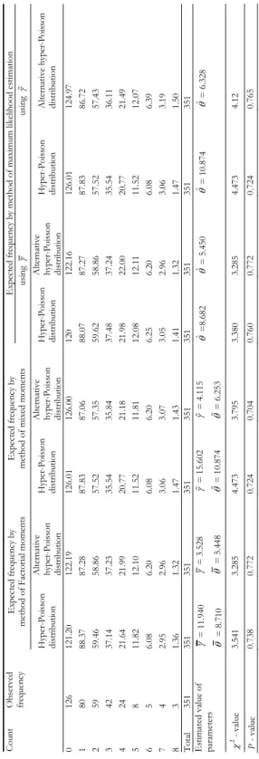
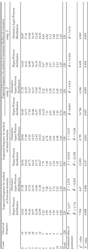
illustrated using two real life data sets, obtained from (Albert, 1991) [or see page 133 of (Hand et al., 1994)] and (Stirrett et.al., 1937) [or Bliss, 1953)] with the help of the mathematical software – MATHCAD and presented in Table 1 and Table 2. From these tables it can be viewed that the AHP distribution gives better fit compared to the hyper-Poisson distribution. Further study on the properties and the comparisons of the estimators of the parameters of the AHP distribution ob-tained in the paper will be published in the sequel.
TABLE 1 Observed dist ribut io n of epilept ic seizure count s (Alber t 1991; Hand et al. 1994) and th e expected frequencies comput
ed using hyper-Poisson dist
ribut
ion and AHP
dis tribution by various methods of estimation Exp ect ed f reque ncy by meth od of ma ximu m likel ih oo d e stimat io n Exp ect ed f reque ncy by me th od of Fa ct or ia l mo me nt s Exp ect ed f reque ncy by method of mixed m oments us in g us in g Co un t Ob se rv ed frequen cy Hyp er-Poi ss on distr ibu tion Alterna tiv e hyp er-Po iss on distr ibu tion Hyp er-Poi ss on distr ibu tion Alterna tiv e hyp er-Po iss on distr ibu tion Hyp er-Poi ss on distr ibu tion Alterna tiv e hyp er-Po iss on distr ibu tion Hyp er-Poi ss on distr ibu tion Altern ativ e h ype r-P oi sson distr ibu tion 0 126 121. 20 122. 19 126. 01 126. 00 120 122. 16 126. 01 124. 97 1 80 88.3 7 87.2 8 87.8 3 87.0 6 88.0 7 87.2 7 87.8 3 86.7 2 2 59 59.4 6 58.8 6 57.5 2 57.3 5 59.6 2 58.8 6 57.5 2 57.4 3 3 42 37.1 4 37.2 3 35.5 4 35.8 4 37.4 8 37.2 4 35.5 4 36.1 1 4 24 21.6 4 21.9 9 20.7 7 21.1 8 21.9 8 22.0 0 20.7 7 21.4 9 5 8 11.8 2 12.1 0 11.5 2 11.8 1 12.0 8 12.1 1 11.5 2 12.0 7 6 5 6.08 6.20 6.08 6.20 6.25 6.20 6.08 6.39 7 4 2.95 2.96 3.06 3.07 3.05 2.96 3.06 3.19 8 3 1.36 1.32 1.47 1.43 1.41 1.32 1.47 1.50 Tota l 351 351 351 351 351 351 351 351 351 Estim ate d v alue of par amet ers = 11. 940 = 8.7 10 = 3.5 28 = 5.4 48 = 15. 602 = 10. 874 = 4.1 15 = 6.2 53 ˆ=8.6 82 ˆ= 5.4 50 ˆ= 10. 874 ˆ= 6.3 28 2 - va lu e 3.54 1 3.28 5 4.47 3 3.79 5 3.38 0 3.28 5 4.47 3 4.12 P - va lu e 0.73 8 0.77 2 0.72 4 0.70 4 0.76 0 0.77 2 0.72 4 0.76 5
TABLE 2 Observ ed dist ribut io n of Corn borers in a field experiment a
rranged in 15 randomized blocks and
th
e expe
cted
frequencies
computed
using hyper-Poisson distribution an
d A H P di str ibuti on by var io us meth ods of esti mati on Exp ect ed f reque ncy by meth od of ma ximu m likel ih oo d e stimat io n Exp ect ed f reque ncy by meth od of F act oria l mom ent s Exp ect ed f reque ncy by meth od of mixed moments us in g us in g Co un t Ob se rv ed frequen cy Hyp er-Poi ss on distr ibu tion Alterna tiv e hyp er-Po iss on distr ibu tion Hyp er-Poi ss on distr ibu tion Alterna tiv e hyp er-Po iss on distr ibu tion Hyp er-Poi ss on distr ibu tion Alterna tiv e hyp er-Po iss on distr ibu tion Hyp er-Poi ss on distr ibu tion Altern ativ e h ype r-P oi sson Distribution 0 19 12.6 5 17.3 8 18.9 6 18.9 6 10.4 5 17.3 5 14.6 2 18.8 7 1 12 16.9 0 16.6 2 19.6 2 17.4 8 14.7 3 16.5 9 16.3 1 17.4 1 2 18 19.2 0 15.7 0 18.7 3 15.9 1 17.6 5 15.6 7 16.8 0 15.8 6 3 18 18.9 7 14.5 3 16.6 1 14.2 3 18.4 0 14.5 1 16.0 7 14.1 9 4 11 16.5 8 13.0 6 13.7 5 12.4 3 16.9 7 13.0 6 14.3 5 12.4 2 5 12 12.9 9 11.3 0 10.6 7 10.5 5 14.0 4 11.3 0 12.0 1 10.5 5 6 7 9.23 9.31 7.79 8.63 10.5 2 9.32 9.47 8.65 7 8 5.99 7.28 5.38 6.78 7.21 7.29 7.05 6.82 8 4 3.59 5.37 3.51 5.09 4.55 5.38 4.97 5.13 9 4 1.99 3.72 2.18 3.64 2.66 3.74 3.33 3.68 10 1 1.03 2.43 1.29 2.48 1.45 2.45 2.12 2.52 11 6 0.50 1.50 0.73 1.60 0.74 1.51 1.29 1.63 Tota l 120 120 120 120 120 120 120 120 120 Estim ate d v alue of par amet ers = 5.6 77 = 3.7 76 = 2.2 78 = 8.5 02 = 12. 015 = 12. 428 = 2.6 33 = 9.6 24 ˆ=8.0 03 ˆ= 8.5 19 ˆ= 13. 410 ˆ= 9.6 74 2 - va lu e 7.95 8 4.67 12.0 95 4.79 9 14.7 86 4.18 6 8.42 8 4.26 9 P - va lu e 0.08 8 0.84 6 0.14 7 0.85 1 0.09 7 0.89 9 0.49 4 0.89 3
ACKNOWLEDGMENTS
The authors would like to express their sincere thanks to the Editor and the anony-mous Referee for carefully reading the paper and for valuable comments. The second au-thor is particularly thankful to UGC, Govt. of India for financial support.
Department of Statistics C. SATHEESH KUMAR
University of Kerala B. UNNIKRISHNAN NAIR REFERENCES
M. ABRAMOWITZ, I.A. STEGUN, (1965), Hand book of Mathematical Functions, Dover, New York. M. AHMAD, (2007), A short note on Conway-Maxwell-hyper Poisson distribution, “Pakistan Journal
of Statistics”, 23, pp. 135-137.
P.S. ALBERT, (1991), A two state Markov mixture model for a time series of epileptic seizure counts, “Biometrics”, 47, pp. 1371-1381.
G.E. BARDWELL, E.L. CROW, (1964), A two parameter family of hyper-Poisson distributions, “Journal of American Statistical Association”, 59, pp. 133-141.
C.I. BLISS, (1953), Fitting the negative binomial distribution to biological data, “Biometrics”, 9, pp. 176-200.
S. CHAKRAVORTHY, (2010), On some distributional properties of the family of weighted generalized
Pois-son distribution, “Communications in Statistics-Theory and methods”, 39, pp.
2767-2788.
E.L. CROW, G.E. BARDWELL, (1965), Estimation of the parameters of the hyper-Poisson distributions, “Classical and Contagious Discrete Distributions”. G. P. Patil (editor), pp. 127-140, Pergamon Press, Oxford.
D.J. HAND, F. DALY, A.D. LUNN, K.J. McCONWAY, E. OSTROWSKI, (1994), A Hand Book of Small Data
Sets, Chapman and Hall, London.
N.L. JOHNSON, A.W. KEMP, S. KOTZ, (2005), Univariate Discrete Distributions, Wiley, New York. C.D. KEMP, (2002), q-analogues of the hyper-Poisson distribution, “Journal of Statistical Planning
and Inference”, 101, pp. 179-183.
C.S. KUMAR, (2009), Some properties of Kemp family of distributions, “Statistica”, 69, pp. 311-316. C.S. KUMAR, B.U. NAIR, (2011), A modified version of hyper Poisson distribution and its applications,
“Journal of Statistics and Applications”, 6, pp. 25-36.
C.S. KUMAR, B.U. NAIR, (2012), An extended version of hyper Poisson distribution and some of its
appli-cations, “Journal of Applied Statistical Sciences”, 19 (To appear).
A.M. MATHAI, H.J. HAUBOLD, (2008), Special functions of applied sciences, Springer, New York. T. NISIDA, (1962), On the multiple exponential channel queuing system with hyper-Poisson arrivals,
“Journal of the Operations Research Society”, 5, pp. 57-66. J. RIORDAN, (1968), Combinatorial identities, Wiley, NewYork.
A. ROOHI, M. AHMAD, (2003a), Estimation of the parameter of hyper-Poisson distribution using negative
moments, “Pakistan Journal of Statistics”, 19, pp. 99-105.
A. ROOHI, M. AHMAD, (2003a), Inverse ascending factorial moments of the hyper-Poisson probability
dis-tribution, “Pakistan Journal of Statistics”, 19, pp. 273-280.
P.J. STAFF, (1964), The displaced Poisson distribution, “Australian Journal of Statistics”, 6, pp. 12-20.
G.M. STIRRETT, G.BEALL, M.TIMONIN, (1937), A field experiment on the control of the European corn
borer, “Pyrausta nubilalis Hubn”. by Beauveria bassiana Vuill. Scient. Agric, 17, pp.
SUMMARY
An alternative hyper-Poisson distribution
An alternative form of hyper-Poisson distribution is introduced through its probability mass function and studies some of its important aspects such as mean, variance, expres-sions for its raw moments, factorial moments, probability generating function and recur-sion formulae for its probabilities, raw moments and factorial moments. The estimation of the parameters of the distribution by various methods are considered and illustrated using some real life data sets.