E-MAIL SPAM FILTERING WITH LOCAL
SVM CLASSIFIERS
Enrico Blanzieri and Anton Bryl
March 2008
E-Mail Spam Filtering with Local SVM Classifiers
Enrico Blanzieri,University of Trento, Italy, and
Anton Bryl
University of Trento, Italy, Create-Net, Italy
March 17, 2008
Abstract
This paper describes an e-mail spam filter based on local SVM, namely on the SVM classifier trained only on a neighborhood of the message to be classified, and not on the whole training data available. Two problems are stated and solved. First, the selection of the right size of neighborhood is shown to be critical; our solution is based on the estimation of the a-posteriori probability of the correct decision, and the resulting algorithm is called highest probability SVM nearest neighbor (HP-SVM-NN). The second problem is the application of the algorithm in practice, and we propose a practical filter architecture based on HP-SVM-NN. Extensive testing is performed on SpamAssassin corpus and TREC 2005 Spam Track corpus, showing that HP-SVM-NN outperforms pure SVM and is applicable in practice. Finally, we explore the locality properties of the two corpora using Sammon’s projection.
1
Introduction
The problem of e-mail spam has gained much attention during the last decade due to both financial losses caused by unsolicited e-mail, and illegal acts (such as online fraud) that exploit spam. Spam filtering is one of the approaches used to stop spam, and the most popular in practice [29]. The existing solutions already achieve very high accuracy. For example, Bratko et al. [7] report their filter to show a spam misclassification rate of 1.17% with a false positive rate of only 0.1%. However, the huge amounts of spam broadcasted today make aiming on increase of the accuracy of the existing algorithms still meaningful. In fact, having a true positive rate, for example, of 99% instead of 98% means half as much spam reaching one’s mailbox.
Since spam filters based on the Na¨ıve Bayes classifier were first proposed in 1998 [22, 24], great number of learning-based filtering techniques appeared. Among them are both general-purpose classifiers, such as k-Nearest Neighbors [2], and application specific algorithms, such as the approach based on the analysis on the reverse paths of e-mail mes-sages proposed by Leiba et al. [19]. For a more detailed discussion of learning-based spam filtering see the survey by Blanzieri and Bryl [3]. One of the learning-based algorithms
applied to spam filtering is the Support Vector Machine (SVM) classifier [8]. SVM were first proposed for spam recognition by Drucker et al. [14] and was shown to outperform many other classification methods on this task [18, 32]. Zhang et al. [32] say, in particular, that using non-linear kernels does not lead to improvement of accuracy of SVM in the case of spam filtering. The SVM classifier has a drawback of high computational cost of re-learning. A solution to this problem was recently proposed by Sculley and Wachman [26], who designed a relaxed online version of the classifier. In the same paper it is shown that SVM is able to reach state-of-the-art classification performance on online spam filtering. A variant of SVM which allows consideration of unequal error costs on the training stage was proposed by Morik et al. [21]. This variant of SVM, which will be referred to as SVM* in this paper, to our best knowledge have not been used for spam filtering before with the exception of the preliminary results of this work [5].
SVM provides a global decision rule independent of the sample which must be classified. However, there is some motivation for building spam filtering upon local decision rules. Spam is not uniform but rather consists of messages on different topics [15] and in different genres [10]. The same considerations apply also to legitimate mail. The existence of algo-rithms which classify e-mail by topic (see, for example, Li et al. [20]) provides evidence of both locality in legitimate mail and the possibility to capture it using bag-of-words feature extraction. The simplest spam filtering method which makes use of locality in the data is k-Nearest Neighbor (k-NN). The k-NN classifier itself was shown to be outperformed by SVM on spam vs. non-spam classification task [18, 32]. Delany et al. [11] proposed k-NN in an online version with a dataset that is built on the fly and showed that its results are comparable to Naive Bayes, which is also outperformed by SVM [32]. This suggests that a more elaborate way of building local decision rules is needed.
An accurate local classification can be achieved by a combination of SVM and k-NN, more precisely by using k-NN for selecting relevant training data for SVM, as was proposed by Blanzieri and Melgani [6] and independently by [31]. This algorithm, which we will fur-ther call SVM nearest neighbor (SVM-NN), is able to achieve a smaller generalization error bound than pure SVM. This theoretical property makes us prefer SVM-NN against other algorithms which combine SVM and k-NN, which are briefly described below. Domeniconi and Gunopulos [12] use the SVM classifier to define a local feature weighting scheme which is further used in k-NN. Sebban and Nork [27] use SVM to select a subset of relevant data for k-NN from the training set. Somewhat similar is the approach proposed by Shen and Len [28], where a new instance is first classified with SVM, and then, if the distance from the separating hyperplane does not exceed a predefined threshold, the sample is re-classified with the k-NN classifier which selects the nearest neighbors not from the whole training set, but only from the set of support vectors. Thus, in this algorithm the SVM classifier is used in particular to select relevant training data for k-NN.
In this paper we present a way to adapt SVM-NN to the task of spam filtering. To achieve this goal we define and evaluate methods of finding the right value of k, to which the algorithm is sensitive, and a practical filter architecture to use the algorithm in practice. In particular, we evaluate two approaches to the selection of k. The first, namely estimation of the optimal size of neighborhood by means of an evaluation set, fails to outperform SVM* on the spam filtering task. The second approach, in which for each message to be classified the algorithm selects the value of k which leads to the highest estimated
a-posteriori probability of the correct decision, proves to outperform SVM and SVM*. This probability-based version of the algorithm, which we call the highest probability SVM nearest neighbor (HP-SVM-NN) classifier, is further used as the core of a practical filtering architecture, which combines a high level of accuracy with reasonable speed. HP-SVM-NN and the practical filter are evaluated on SpamAssassin corpus and TREC 2005 Spam Track corpus respectively. Results of the comparison of HP-SVM-NN with other methods on SpamAssassin corpus were partly presented at CEAS 2007 [5].
The paper is organized as follows. Section 2 gives a detailed description of the HP-SVM-NN classifier. Section 3 is dedicated to the experiments used to evaluate this algorithm. In Section 4 we describe an architecture for a practical spam filter based on HP-SVM-NN, and in Section 5 we address the evaluation of this architecture. Section 6 gives some explanation of the results of the experiments by showing the presence of locality in the vectors of features extracted from e-mail messages. Finally, Section 7 is the conclusion.
2
The Classification Algorithms
In order to present SVM-NN and HP-SVM-NN we need first to describe the SVM classifier.
2.1 Support Vector Machines
SVM [8] is a state of the art classifier, whose detailed description can be found, for example, in the book by Cristianini and Shawe-Taylor [9]. Let there be n labeled training samples that belong to two classes. Each sample xi is a vector of dimensionality d, and each label
yi is either 1 or −1 depending on the class of the sample. Thus, the training data set can
be described as follows:
T = ((x1, y1), (x2, y2), ..., (xn, yn)),
xi∈ Rd, yi ∈ {−1, 1}.
Given these training samples and a predefined transformation Φ : Rd → F , which maps the features to a transformed feature space, the SVM classifier builds a decision rule of the following form: ˆ y(x) = sign L X i=1 αiyiK(xi, x) + b ! ,
where K(a, b) = Φ(a)·Φ(b) is the kernel function and αiand b are selected so as to maximize
the margin of the separating hyperplane. A predefined parameter, cost factor C, is used to establish a tradeoff between margin size and a training error penalty.
It is also possible to get the result not in the binary form, but in the form of a real number, by dropping the sign function:
y0(x) =
L
X
i=1
αiyiK(xi, x) + b,
This real-number output can be used, in particular, for estimating the posterior probability of the classification error. In fact, some applications require not a binary classification
Algorithm: The SVM Nearest Neighbor Classifier Input: sample x to classify;
training set T = {(x1, y1), (x2, y2), ...(xn, yn)};
number of nearest neighbors k. Output: decision yp ∈ {−1, 1}
1: Find k samples (xi, yi) with minimal values of K(xi, xi) − 2 ∗ K(xi, x)
2: Train an SVM model on the k selected samples
3: Classify x using this model, get the result yp
4: return yp
Figure 1: The SVM Nearest Neighbor Classifier: pseudocode.
decision, but rather posterior probabilities of the classes P (class|input). SVM provides no direct way to obtain such probabilities. Nevertheless, several methods of approximation of the posterior probabilities for SVM are proposed in the literature. In particular, Platt [23] proposed the approximation of the posterior probability of the positive class with a sigmoid:
ˆ
P (y = 1|y0) = 1
1 + eAy0+B (1)
where A and B are parameters obtained by fitting on an additional data set. Platt observes that for the SVM classifier with the linear kernel it is acceptable to use the same data both for training the SVM model and for fitting the sigmoid. The description of the procedure of fitting the parameters A and B can be found in Platt’s original publication [23].
In some practical tasks it is necessary to consider unequal error cost and thus to change the balance between false positives and false negatives. A simple way to adjust the balance between the two types of errors with SVM is to apply different thresholds to y0(x). Another approach was proposed by Morik et al. [21]. In this approach, different cost factors C+
and C− are ascribed to the training errors from the two classes during the training process.
SVM with the balance between the error types adjusted in this way will be called SVM* in this paper.
2.2 The SVM Nearest Neighbor Classifier
SVM-NN [6] is a local SVM classifier obtained by combining SVM with k-NN. The k-Nearest Neighbors Classifier (k-NN) makes the classification decision by counting the representatives of each class in the k-neighborhood of the instance x to be classified. The k neighborhood of x is the set of k instances from the training data which lie most closely to x in terms of the chosen distance function. The decision is taken in favor of the class which has the majority of representatives in the the k-neighborhood of x.
In order to classify a sample x, SVM-NN first selects the k nearest samples to the sample x, and then uses these k samples to train an SVM that is used to perform the classification. The pseudocode of the basic version of the algorithm is given in Figure 1. Samples with minimal values of K(xi, xi) − 2K(xi, x) are the closest samples to the sample x in the
transformed feature space, as can be seen from the following equality: ||Φ(xi) − Φ(x)||2 = Φ2(xi) + Φ2(x) − 2Φ(xi) · Φ(x) =
Algorithm: Parameter Estimation for the SVM* Nearest Neighbor Classifier Input: training set T = {(x1, y1), (x2, y2), ...(xn, yn)}
set of possible values of th number of nearest neighbors K = {k1, k2, ..., kN};
percentages of data used for training and validation ρ1 and ρ2, ρ1+ ρ2 ≤ 1.
Output: best number of nearest neighbors kbest.
using an external function: f is a performance measure to optimize.
preliminary calculations: prepare a matrix M , mij = K(xi, xj), i, j = 1..n, where K is
the SVM kernel used.
1: Select randomly T1 ⊂ T and T2 ⊂ T , T1T T2= ∅, |T|T |1|= ρ1, |T|T |2| = ρ2
2: fbest= 0 # the best performance achieved at the moment.
3: for k in (set of possible values of k) do
4: Classify all samples in T2 with SVM*-NN using T1 as training data and k as the number
of nearest neighbors; calculate the performance fk using the measure f .
5: if fk > fbest then
6: fbest= fk
7: kbest= k
8: end if
9: end for
10: kbest= kbest/ρ1 # scale kbest by |T|T |1|
11: return kbest.
Figure 2: Finding the right value of k for the SVM*-NN classifier using training and vali-dation on subsets of the training data.
= K(xi, xi) + K(x, x) − 2K(xi, x)
This algorithm is able to achieve a smaller generalization error bound in comparison to global SVM because of a bigger margin and a smaller ball containing the points [6]. However, the parameter k is critical and needs a careful estimation. Blanzieri and Melgani [6] showed that for remote sensing data using a validation set for estimating the parameter k for the SVM-NN classifier leads to good results. Therefore, we decided to find the value of k by training and validating the classifier with different values of k on two subsets of the training data, and then selecting the value which led to the highest performance. If SVM* is used for building the local rule instead of plain SVM, such a local classifier will be referred to as SVM*-NN. The pseudocode for estimation of k for SVM*-NN is given in Figure 2. Scaling of the selected value of k is needed because, given that internal training and validation sets are obtained by random sampling of T , the same sphere in the feature space will contain on average 1/ρ1 times fewer messages from the internal training set T1
than from the whole training set T . For SVM-NN the optimal threshold for achieving the desired balance between the errors should be estimated as well in the same way as the parameter k.
2.3 The Highest Probability SVM Nearest
Algorithm: The Highest Probability SVM Nearest Neighbor Classifier Input: sample x to classify;
training set T = {(x1, y1), (x2, y2), ...(xn, yn)};
set of possible values for the number of nearest neighbors K = {k1, k2, ..., kN};
parameter R for adjusting the balance between the two types of errors. Output: decision yp ∈ {−1, 1}
1: Order the training samples by the value of K(xi, xi) − 2 ∗ K(xi, x) in ascending order.
2: MinErr = 1.0
3: Value = 0
4: if the first k1 values are all from the same class c then
5: return c
6: end if
7: for all k in (set of possible values of k) do
8: Train SVM model with equal error costs on the first k training samples in the ordered list.
9: Classify x using the SVM model, get the result y0.
10: Classify the same training samples using this model.
11: Fit the parameters A and B for the function ˆP (y = 1|y0) which estimates the probability of positive class.
12: if 1 − ˆP (y = 1|y0) < MinErr then
13: MinErr = 1 − ˆP (y = 1|y0)
14: Value = 1
15: end if
16: if ˆP (y = 1|y0) ∗ R < MinErr then
17: MinErr = ˆP (y = 1|y0) ∗ R
18: Value = −1
19: end if
20: end for
21: return Value
Figure 3: The Highest Probability SVM Nearest Neighbor Classifier: pseudocode.
HP-SVM-NN is based on the idea of selecting the parameter k for local SVM from a predefined set K = {k1, ..., kN} separately for each sample x which must be classified.
The pseudocode of the algorithm is presented in Figure 3. To classify a sample, the algorithm first performs the following actions for each considered k: k training samples nearest to the sample x are selected; an SVM model is trained on these k samples; the estimation of the class probability function is built as proposed by Platt [23]. To estimate the probabilities of the classes, the same k samples are classified using the SVM model, and the output is used to fit the parameters A and B in the equation (1). The sample x is then classified using the SVM model, and the real-number output of the model is used to calculate the estimated probabilities of the classes ˆP (y = 1|y0) and ˆP (y = −1|y0) = 1 − ˆP (y = 1|y0). Thus, for each k the algorithms provides two decisions with estimated probabilities of errors (probability of the positive class is the error probability for the decision in favor of the negative class, and vice versa), which gives 2×N decision in total. Among those, the answer
with the lowest probability of error (in other words, with the highest estimated probability of the correct decision, hence the name of the classifier) is chosen. An additional parameter R can be used to adjust the balance between false positives and false negatives. In this case, the probability of error for the negative answer must be not just lower than the probability of error for the positive answer, but at least R times lower in order to be selected. If false positives are less desirable than false negatives, R < 1 should be used. The architecture of the algorithm, based on probabilistic decisions, makes it useless to create a separate version using SVM* instead of SVM, so there is only one variant of HP-SVM-NN.
We must mention that from the point of view of speed HP-SVM-NN is not the same as N runs of basic SVM-NN classifier, because the costly operation of distance calculation is performed only once for each classified sample. In one special case, namely when with the smallest considered value of k all the nearest neighbors belong to the same class, additional optimization is used. More precisely, in this simple case the estimate of posterior probability of the class from which the neighboring samples come is equal to 1.0, thus the error estimate is equal to 0 and no lower value can be reached. If such a case occurs, the decision is taken immediately and no further search is performed. We will call such samples ‘easy’, and the samples for which the full search among the possible values of k is performed we will call ‘hard’.
2.4 Feature Extraction for Spam Data
In the commonly used Simple Mail Transfer Protocol (SMTP), a message consists of a header and a body. The message header is a set of named fields, each containing particular information about the message: the subject line, the address of the sender, the addresses of the receivers, the date, and so on. The message body is the content of the message.
To transform an e-mail message into a vector of numbers which can be processed by the classification algorithms, a feature extraction procedure is needed. A simple way to extract features for any of the discussed algorithms is the following. Each part of the message, namely the message body and each field of the message header, is represented as a bag of words or, in other words, as an unordered set of strings (tokens) separated by spaces. Presence of a particular token in a particular part of the message is considered a binary feature fi∈ {0, 1} of the message. Then, the d features with the highest Document
Frequency or Information Gain (the choice will be specified separately in each case) are selected. Thus, each message is represented with a vector of d binary features.
Document Frequency (DF) is defined as follows:
DF (fi) = |{mj|mj ∈ M and fi occurs in mj}|,
where M is the set of all training messages and fi is a binary feature (for example “the
word free is present in the message”).
Information Gain (IG) is defined as follows:
IG(fi) = X c∈{cspam,cleg} X f ∈{fi,¬fi} ˆ P (f, c) log P (f, c)ˆ ˆ P (f ) · ˆP (c) ,
where cspam and cleg are the labels of spam class and legitimate mail class respectively, fi is
of the feature fi (for example “the word free is NOT present in the message”), and ˆP is
probability estimated by frequency.
3
Evaluation of the Classification Algorithms
In order to evaluate the algorithms on spam data we first establish a baseline for the comparisons, then we proceed with preliminary experiments that eventually lead to the definition of the HP-SVM-NN classifier which is finally evaluated in terms of ROC curves.
3.1 Establishing a Baseline
To establish a baseline for the comparisons, we reproduced the experiments with the SVM classifier, presented by Zhang et al. [32]. The linear kernel is used for SVM in all cases, following the observation by Zhang et al. that changing the kernel gives no increase in accuracy for spam filtering. Evaluation in the same paper showed that SVM undoubtedly outperforms k-NN, so we did not consider k-NN in our comparisons. The evaluation con-sists in ten-fold cross-validation on the SpamAssassin corpus1. The corpus contains 4150 legitimate messages and 1897 spam messages. The same random splitting of the data into ten folders was used in all cross-validations performed for this study. The implementation of SVM used for this and further experiments is a popular set of open-source utilities called SVMlight2 [17].
The performance measure used by Zhang et al. is Total Cost Ratio (TCR), proposed by Androutsopoulos et al. [1], which allows to consider unequal error cost. TCR is defined as follows:
T CR = nS
λ · nL→S + nS→L
,
where nS is the total number of spam messages, nL→S is the number of legitimate messages
classified as spam, nS→L is the number of spam messages classified as legitimate, and λ
is the relative cost of misclassification of a legitimate message and misclassification of a spam message. TCR for cross-validation was computed as the average of the values of TCR obtained for the ten folders, as done by Zhang et al. Apart from this, we computed also the harmonic mean. The reason is the following: the average TCR depends not only on the average weighted error rate, but also on the difference between the weighted error rates for different folders (the greater the difference, the higher the value), which can be misleading. At the same time it is easy to show that the harmonic mean will provide a value which depends only on the average weighted error rate. The following names will be used for this two measures on figures: TCRn for the average of the ten values TCR with λ = n, and TCRn * for the harmonic mean. Following the experiment of Zhang et al., we used λ = 9 and b0 = 0.48, where b0 is the fixed threshold used to convert the real-number output of SVM into a binary decision (see Section 2.1).
The results can be seen in Figure 4a (the curve labeled SVM). They are close to those provided by Zhang et al., though evidently not exactly the same, because the partitioning
1
Available at: http://spamassassin.apache.org/publiccorpus/
2
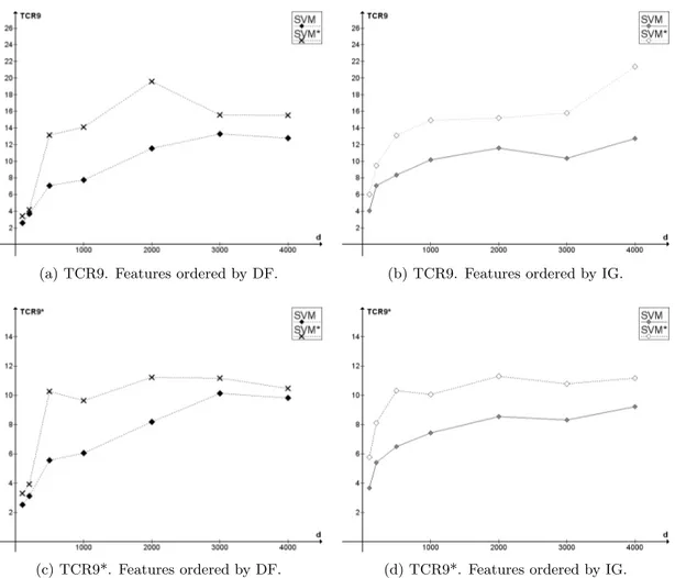
(a) TCR9. Features ordered by DF. (b) TCR9. Features ordered by IG.
(c) TCR9*. Features ordered by DF. (d) TCR9*. Features ordered by IG.
Figure 4: Establishing a baseline. Comparison of performance of SVM with a fixed threshold equal to 0.48 (SVM) and SVM with the relative cost passed as a parameter to the software (SVM*) in terms of TCR.
of the data is random and thus cannot be reproduced. For example, with features ordered by document frequency the results for the numbers of features equal to 1000 and 3000 are 7.06 and 13.29 in our experiment and about 7.7 and 12.3 on the graph given by Zhang et al.
In order to establish a better baseline, we then compared two variants of SVM: SVM with a fixed threshold (as described above), further called simply SVM, and SVM* (see Section 2.1). SVM* is directly supported by SVMlight, which allows the user to pass C+
C−
as an additional parameter. The kernel is linear in both cases. Figure 4 shows the results of the comparison in terms of TCR and TCR*. As we can see, SVM* has a doubtless advantage both with DF and IG feature ordering and with both ways of computing TCR. Accordingly, SVM* will further be used as a quality baseline for the experiments presented in this section.
3.2 Preliminary Experiments
The outline of the preliminary experiments presented in this subsection is as follows. The first experiment compares SVM*-NN with SVM* and suggest that estimation of the pa-rameter k for SVM*-NN using an evaluation set does not allow SVM*-NN to outperform SVM*. This motivates the second experiment, which addresses the question of whether there are suitable values of k at all. The positive results of this experiment show that using local SVM is promising for spam filtering, but a totally different approach to the selection of k is needed. This leads to the definition of HP-SVM-NN, which is preliminarily evaluated in the third experiment.
3.2.1 Experimental Procedures
Experiment 1. SVM*-NN vs. SVM*. In this experiment we compared SVM*-NN and SVM*. SVM-NN is not considered in the comparisons in this paper. The experimental results on SVM-NN were presented previously [4], and show that it has performance com-parable to that of SVM, which leaves no chance for SVM-NN to outperform SVM*. For SVM*-NN the following parameters were used: K = {30, 50, 100, 150, 200, 250, 300, 350, 400, 500, 600, 700, 850, 1000, 1200, 1400, 1650, 1900, 2200, 2500, 2900, 3300, 3800, 4300, 4800}; ρ1 = 0.9; ρ2 = 0.1; f = TCR9. The following values of the number of features d
were used: 100, 200, 500, 1000, 2000, 3000, 4000.
Experiment 2. Is there a good value for k? The question answered by this experiment is: are there at all values of k which allow SVM*-NN to outperform SVM*? The data in each of the ten folders used for cross-validation was classified with SVM* and with SVM*-NN with all the considered values of k in order to see whether any value of k allows SVM*-NN to outperform SVM*, and whether this value is invariant for different folders. K, ρ1 and ρ2 are the same as in Experiment 1. The following values of the number
of features d were used: 500, 1000.
Experiment 3. Preliminary evaluation of HP-SVM-NN. In this experiment we compared HP-SVM-NN with the SVM classifier in terms of overall error rate, false positive rate and false negative rate using equal error costs (in case of equal error cost SVM and SVM* are equivalent). In this experiment we used the same set K as in the two previous experiments, but with each value scaled by 1/ρ1 (for SVM*-NN the same scaling is done
by the procedure of estimation of k, as explained in Section 2.2). The following values of the number of features d were used: 100, 200, 500, 1000, 2000, 3000, 4000.
3.2.2 Results
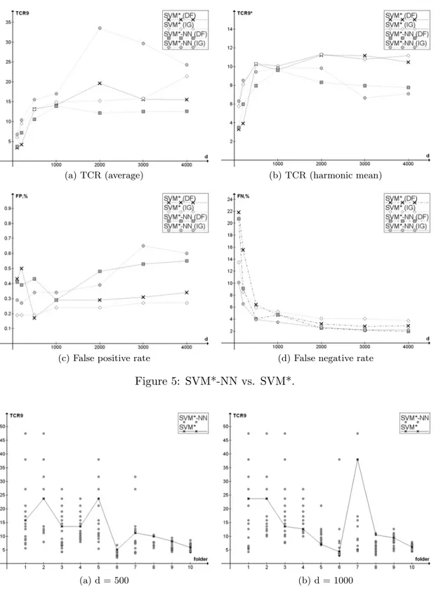
The results of the comparison between SVM* and SVM*-NN (Experiment 1) are presented in Figure 5. The results in terms of average TCR (Figure 5a) are misleadingly optimistic. However, the comparison in terms of more stable harmonic mean of TCR (Figure 5b) shows that SVM* performs clearly better. This suggests, that local SVM classifier with the number of nearest neighbors estimated using an evaluation set is not effective on spam filtering. This initial failure led to the design of Experiment 2.
Figure 6 shows the results of Experiment 2. We can see, that for each folder there is a value of k which allows SVM*-NN to outperform SVM*. Moreover, in most cases there
(a) TCR (average) (b) TCR (harmonic mean)
(c) False positive rate (d) False negative rate
Figure 5: SVM*-NN vs. SVM*.
(a) d = 500 (b) d = 1000
Figure 6: Is there a good k? TCR is plotted separately for each folder, so this is neither average nor harmonic mean of the calculated values, but the values themselves. IG is used for ordering features.
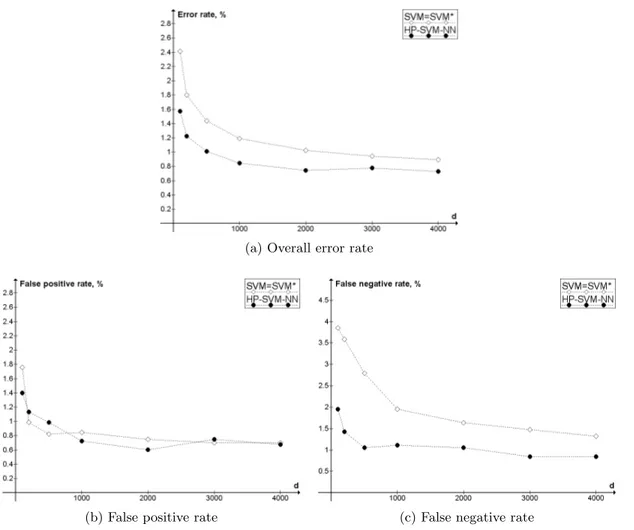
(a) Overall error rate
(b) False positive rate (c) False negative rate
Figure 7: Preliminary evaluation of HP-SVM-NN. d is the number of features. R = |C+|
|C−| = 1.
are several such values, so even a suboptimal estimation of k could be acceptable. At the same time, this values vary greatly for different folders. For example, with d = 1000 the values vary approximately from 600 to 3000, and there is only one pair of folders for which the values were the same. This implies that the optimal size of neighborhood is highly dependant on the particular set of data, suggesting that parameter estimation using evaluation set is a wrong choice for this task, and therefore a different procedure of selecting k is needed. This result motivates the definition of HP-SVM-NN (see Section 2.3).
In Figure 7 the results of the preliminary comparison of HP-SVM-NN and SVM (Ex-periment 3) are presented. It shows that HP-SVM-NN is able to outperform SVM at least in the case of equal error costs. The evaluation of the significance of the advantage of HP-SVM-NN in terms of overall error rate, performed using Wilcoxon signed-rank test with α = 0.05, showed that the difference is significant for d below or equal to 2000, and not significant for d = 3000 and d = 4000. Figure 7b,c shows that with equal error costs the classifiers have close performance in terms of false positives, but the HP-SVM-NN classifier is invariably better in term of false negatives. After obtaining this encouraging preliminary result we passed to a more thorough evaluation of HP-SVM-NN.
Number of TPR with FPR = 0.01 TPR with FPR = 0.005 features SVM* HP-SVM-NN SVM* HP-SVM-NN 100 0.930 (0.00082) 0.964 (0.00034) 0.892 (0.00061) 0.926 (0.00308) 200 0.964 (0.00027) 0.986 (0.00010) 0.946 (0.00030) 0.973 (0.00141) 500 0.976 (0.00014) 0.989 (0.00010) 0.959 (0.00970) 0.981 (0.00031) 1000 0.983 (0.00011) 0.992 (0.00009) 0.968 (0.00021) 0.984 (0.00030) 2000 0.987 (0.00011) 0.995 (0.00005) 0.979 (0.02035) 0.989 (0.00025) 3000 0.989 (0.00014) 0.995 (0.00004) 0.981 (0.01018) 0.988 (0.00041) Table 1: Comparison of SVM* and HP-SVM-NN: selected points. Variance is given in brackets.
3.3 Evaluation of HP-SVM-NN in Terms of ROC Curves
Unlike SVM*-NN, which requires performing the parameter estimation separately for each value of relative error cost, HP-SVM-NN allows building a ROC curve in reasonable time. Thus, considering that ROC curves are more informative than TCR, we decided to use them for measuring the accuracy in this experiment. As the comparison between SVM and SVM* in terms of ROC curves is inconclusive (see Figure 8), it is meaningful to compare HP-SVM-NN with both SVM and SVM* when using ROC curves.
3.3.1 Experimental Procedure
In this experiment we compared HP-SVM-NN, SVM and SVM* in terms of ROC curves, thus considering the unequal error costs. The following set K of 12 values was used: {50, 150, 250, 350, 500, 700, 1000, 1400, 2000, 2800, 4000, 5400}. We used a smaller set than in the previous experiments to make the algorithm faster. The values of the number of features were the same as in the previous experiment. In order to build the ROC curves, for HP-SVM-NN the parameter R (see Figure 3) is changed from 1.5 ∗ e−25 to 1.5 ∗ e25 with uniform steps on a logarithmic scale; for SVM* the parameter C+
C− is changed in the
same way; and for SVM the threshold applied to the output is changed from -4 to 4 with step 0.01. For all the parameters of SVM* except C+
C− and for all the parameters of SVM
the default values are used as implemented in SVMlight. Inside the HP-SVM-NN the SVM classifier is also used with default parameters in all cases.
3.3.2 Results
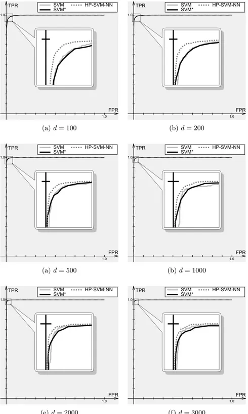
In Figure 8 the comparison HP-SVM-NN with SVM and SVM* in terms of ROC curves is presented. In Table 1 the values of true positive rate of the classifiers are compared with the false positive rates of 0.01 and 0.005 (false positives are obviously much more expensive in the task of spam filtering, so the points with low false positive rate are of particular practical interest). SVM is not reported in the table because, as can be seen in Figure 8, on low false positive rates it is never better than SVM*.
We can see that HP-SVM-NN performs better in all cases. Thus, from the point of view of accuracy, HP-SVM-NN is a viable solution to the problem of selecting locality size for spam filtering with local SVM. Note that, however small may seem the difference, the true
(a) d = 100 (b) d = 200
(a) d = 500 (b) d = 1000
(e) d = 2000 (f) d = 3000
Figure 8: Comparison of SVM, SVM* and HP-SVM-NN in terms of ROC curves. TPR is the true positive rate, FPR is the false positive rate, and d is the number of features. Positive class is spam, negative class is legitimate mail.
positive rate of 0.988 instead of 0.981 (the case with 3000 features and the false positive rate of 0.005) means actually that 37% less spam finally reaches the user’s mailbox.
4
A Practical Spam Filter Based on HP-SVM-NN
As a classification task, spam filtering has a peculiarity which must be addressed when designing a practical solution, namely frequent insertion of new samples to the training data, which leads to both need for constant update of the classification model and rapid growth of the number of training samples. In this section we describe an architecture which allows to utilize the HP-SVM-NN classifier in practice, processing the data at a reasonable speed.
The HP-SVM-NN classifier obviously performs slower (and consumes more memory) with the increase of the amount of training data. This leads to a need for pre-selection of data before training. The necessity of coping with the changeability of e-mail suggests a simple but presumably meaningful way of doing such pre-selection, namely to apply a time window of dimension W to the data, in other words, to use only the W most recent messages for training.
The feature extraction is performed in the same way as in section 2.4, but using only the messages in the current window. Information Gain is used for feature ordering. We must mention that the Information Gain is a measure quite convenient for online re-training. For each feature it is enough to know at every moment the amount of spam and legitimate messages in which this feature occurs in the current window. From this two values, which are easy to maintain incrementally, and the total number of messages of each class in the training data it is easy to calculate the Information Gain.
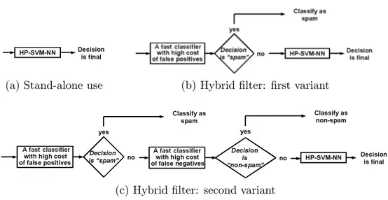
With a large window size and/or number of features the HP-SVM-NN classifier can be too slow to be used in practice. In such a case instead of using HP-SVM-NN stand-alone (Figure 9a) it makes sense to combine it with a faster algorithm, so that only a small subset of messages are classified by HP-SVM-NN. This will allow to profit from its high accuracy without loosing too much in classification speed. If the system receives much spam and comparatively small amount of legitimate mail, the following procedure can be used to classify a message. First, the message is classified using a faster classification algorithm, for example Na¨ıve Bayes, with the cost of false positives set to a very high value. If it is classified as spam, this decision is final; if it is classified as legitimate mail, the final decision is taken by re-classifying this message with HP-SVM-NN. The scheme of this procedure is shown on Figure 9b. If the system receives large amount of both spam and legitimate mail, the following, a bit more complicated, procedure can be used to classify a message. First, as in the previous case, a fast classifier with the cost of false positives set to a very high value is applied to the message, and if it is classified as spam, no further check is performed. If it classified as legitimate mail, this decision is re-checked by the same classifier, but this time with high cost of false negatives. If the answer is again “legitimate mail”, this decision is final, else the HP-SVM-NN classifier is used to make the final decision. The scheme of this procedure is shown on Figure 9c.
(a) Stand-alone use (b) Hybrid filter: first variant
(c) Hybrid filter: second variant
Figure 9: Using HP-SVM-NN: stand-alone or in combination with a faster classifier. The first variant of the hybrid filter is for the systems which receive much spam and small amount of legitimate mail. The second variant is for the systems which receive huge number of both spam and legitimate mail.
5
Evaluation of the HP-SVM-NN Spam Filter
5.1 Assessing the Accuracy
5.1.1 Experimental Procedures
For the evaluation of the final architecture we decided to choose TREC 2005 Spam Track corpus, which has two major advantages over the SpamAssassin corpus. Firstly, it contains much more data (39399 legitimate messages and 52790 spam messages); secondly, it pre-serves the time order of the messages, which allows to effectively simulate online testing and thus to evaluate classifiers in more realistic conditions.
In our experiment, each message except the first W was classified with HP-SVM-NN trained on the W previous messages. Then, the results were presented as ROC curves, with spam as positive class and legitimate mail as negative class. The SVM and SVM* classifier, as implemented in the SVMlight package, were used for comparison. Feature extraction for SVM and SVM* was performed in exactly the same way as for HP-SVM-NN, and the same window size was used for all the three algorithms in each case. It would be interesting also to compare HP-SVM-NN with relaxed online SVM which was recently proposed by Sculley and Wachman [26]. However, relaxed online SVM relies on a seriously different procedure for feature extraction, and so the design of a fair comparison is complex, therefore we leave such comparison to future work.
The HP-SVM-NN classifier was implemented in C++ with the modules of SVMlight used for training SVM models. The following values of the window size W were used: 2000, 3000. For W = 2000 the following 9 possible values of k were used: 100, 200, 300, 500, 700, 1000, 1300, 1650, 2000. For W = 3000 each value in the same set was scaled by 1.5.
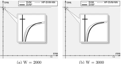
(a) W = 2000 (b) W = 3000
Figure 10: Comparison of SVM, SVM* and HP-SVM-NN with a time window. TPR is the true positive rate, FPR is the false positive rate, and W is the window size. The number of features d = 500. Positive class is spam, negative class is legitimate mail. On this data SVMlight did not produce the points with high false positive rate for SVM*, as can be seen on the figures.
Window TPR with FPR = 0.01 TPR with FPR = 0.005 size SVM HP-SVM-NN SVM HP-SVM-NN 2000 0.973 0.979 0.960 0.968 3000 0.976 0.983 0.964 0.973 Table 2: Comparison of SVM and HP-SVM-NN: selected points.
5.1.2 Results
The results are presented in Figure 10. The number of features is d = 500. On this data SVMlight did not produce the points with high false positive rate for SVM*, probably due to the insufficient precision of floating-point variables. This, however, does not imply that the method should be discarded, because in spam filtering only the case of low false positive rate is practically interesting. Selected points are compared in Table 2. In this experiment, as it can be seen in Figure 10, SVM outperforms SVM* on low false positives, and so only the results for SVM are presented in the table. It is interesting to mention the difference in the relative performance of SVM and SVM* in the experiments on SpamAssassin corpus and on Spam Track corpus, which is probably due to the fact that the two corpora are differently unbalanced: in SpamAssassin corpus legitimate mail constitutes the majority of messages, while in Spam Track corpus it is outnumbered by spam. We can see that HP-SVM-NN is able to outperform both variants of the pure SVM classifier. Thus, the results on Spam Track corpus are consistent with the results on SpamAssassin corpus.
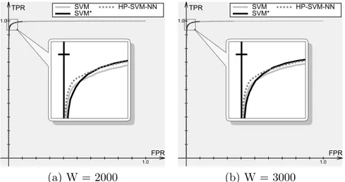
(a) W = 2000 (b) W = 3000
Figure 11: Comparison of SVM, SVM* and HP-SVM-NN with a time window using the data only from the message headers. TPR is the true positive rate, FPR is the false positive rate, and W is the window size. The number of features d = 500. Positive class is spam, negative class is legitimate mail.
Window TPR with FPR = 0.01 TPR with FPR = 0.005 size SVM HP-SVM-NN SVM HP-SVM-NN 2000 0.966 0.972 0.955 0.962 3000 0.968 0.974 0.957 0.965
Table 3: Comparison of SVM and HP-SVM-NN on headers only: selected points.
5.2 Assessing the Accuracy on Headers Only
Image spam, which constitutes a large part of spam e-mail today, requires special attention. It is certainly possible to define a image-based kernel for HP-SVM-NN, but this is a topic for a separate investigation. However, pure SVM is known to be able to distinguish quite accurately between spam and legitimate messages using only message headers, without any reference to the message content, be it a text or an image [32]. Therefore, it is interesting to see, with which level of accuracy HP-SVM-NN can perform the same task.
5.2.1 Experimental Procedures
This experiment is exactly the same as the previous one with W , with the only difference: features are extracted only from the message headers, while the bodies are completely skipped.
5.2.2 Results
The results of this experiment are presented in Figure 11, and selected points are compared in Table 3. SVM* is not presented in the table because, as the figure shows, on low false positives SVM performs better. We can see, that the accuracy of all the three methods on headers only is quite high, and that HP-SVM-NN is more accurate then the other two
Min. time (s) Max. time (s) Avg. time (s) Classification of a message < 0.01 1.532 0.20 Classification of an ‘easy’ message < 0.01 0.011 < 0.01
Classification of a ‘hard’ message 0.21 1.532 0.45 Substitution of a message in the window 0.14 1.88 0.18 Table 4: Time in seconds needed for the operations of the filter. The number of features d = 500, the window size W = 2000. 49761 easy messages and 40428 hard messages were classified.
on low false positives, though on low false negatives SVM* has the same (with W = 2000) or even somewhat better (with W = 3000) performance. This suggests that image spam will be recognized with reasonable accuracy by header analysis only, assuming that the characteristics of the headers of image spam messages are not totally different from the usual spam. However, building a special kernel for image spam, or using some kind of fast feature extraction from images [13, 30], is an interesting direction for future work, as it seems that the images in spam also consist of local groups, and a local classifier which considers images could be even more accurate.
5.3 Assessing the Speed
The goal of this experiment was to measure the speed of the filter and thus to assess the feasibility of its practical use.
5.3.1 Experimental Procedures
In this experiment we measured the minimal, maximal, and average time required by the filter based on HP-SVM-NN to classify a sample and to substitute one message in the window of training data. We also measured separately the average speed of classification of ‘easy’ and ‘hard’ messages (see Section 2.3). All the data and all the software was exactly the same as in the experiment in subsection 5.1. Window size W was taken equal to 2000. For measuring the speed of the algorithm we used a personal computer with CPU speed of 1600MHz and 768MB of memory, running under Windows XP.
5.3.2 Results
The results are presented in Table 4. They suggest that the algorithm is a feasible server-side solution. Average classification time of 0.2 seconds means classifying 300 messages, which is more or less the daily norm received by each of the authors, in one minute. If all the new messages are added to the training data one by one, this addition will take a bit less time than classification itself, 0.18 seconds per message. It is necessary to stress here that, firstly, the presented results are obtained on a computer which is slower than an average modern server, and, secondly, there are methods of training linear SVM faster than with SVMlight [16], so there are still ways to improve the implementation.
In the cases when the speed of HP-SVM-NN standalone is not sufficient, a combination with a faster classifier may be used as shown on Figure 9b,c. Let a system receive n1 easy
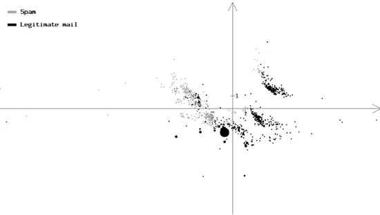
Figure 12: The Sammon’s projection of a 20% subset of SpamAssassin corpus. The original 100-dimensional space contains the messages represented as vectors of 100 binary bag-of-words features with the highest Information Gain. The area of each circle is proportional to the number of messages mapped to the corresponding vector of features. SSammon = 0.20018
messages and n2 hard messages in a given period of time, and let HP-SVM-NN require time
t1 to classify an easy message and time t2 to classify a hard message on this system. Let
there be a faster classifier which is able to filter out n01easy messages and n02hard messages with an average classification time per message t0. Then the scheme in Figure 9b will gain the following speed-up of
Ta
Tb
= n1t1+ n2t2 t0(n
1+ n + 2) + t1(n1− n01) + t2(n2− n02)
Obviously, the speed-up will be greater than 1 if and only if the following inequality is satisfied: t0 < n 0 1t1+ n02t2 n1+ n2 .
For example, with the characteristics of the system described in the experiment above, a combination with a fast filter able to filter out accurately 50% of both hard and easy messages with a classification speed of 0.05 per message will gain a speed-up of 1.33. Similar considerations may be applied also to the scheme in Figure 9c.
6
The Locality Phenomenon in E-Mail
The success of HP-SVM-NN suggests that the data used in our experiments is such that local algorithms can have an advantage. Accordingly, it is interesting to see, whether this locality can be somehow captured by analysis of the data.
(a) Whole messages. SSammon = 0.29836
(b) Headers only. SSammon = 0.30058
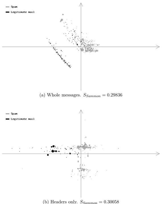
Figure 13: The Sammon’s projections of the first 1000 messages of Spam Track corpus. In both cases the original 100-dimensional space contains the messages represented as vectors of 100 binary bag-of-words features with the highest Information Gain. The area of each circle is proportional to the number of messages mapped to the corresponding vector of features.
One way to get an informal preliminary answer about the presence or the absence of locality in the data is to visualize the data with the Sammon’s projection. The Sammon’s projection [25] is a method of mapping multidimensional objects into a space of lower dimensionality. The method minimizes an error function called the Sammon’s stress, which is defined as follows: SSammon = 1 m P i,j=1 i<j d∗ij m X i,j=1 i<j (d∗ij − dij)2 d∗ij
where m is the number of points mapped, d∗ij is the distance between the ith and jth vectors in the multidimensional space, and dij is the distance between their projections. We used
the implementation of the Sammon’s projection provided by the R software environment3. If the data consists of separate dense groups of samples, this will be seen on the projection. We calculated the Sammon’s projection’s of a 20% subset of the SpamAssassin corpus, of the set of the first 1000 messages of Spam Track corpus, and of the set of headers of the same 1000 messages. Subsets of the corpora was used instead of the whole corpora in order to decrease the amount of memory needed to build the projection. In each case the messages were represented as vectors of 100 features with the highest Information Gain.
In Figures 12 and 13 the Sammon’s projections of the described three sets of data are presented. We can see that in all the three cases the data consists of quite well-distinguishable parts, and most of such separate parts include both spam and legitimate mail. This supports the intuition that local rules for separating spam from legitimate mail can be more effective than global rules. It is important to mention that Sammon’s projection only preserves information about distances between samples, and does not allow reasoning about local or global linear separability of the classes.
There are probably three aspects of the classification problem which are affected by leveraging locality. The first is the accuracy of the decision rule, and we have shown in this paper that consideration of locality increases it. The effect on the other two is not yet explored. The second is capability of adjusting the balance between false positives and false negatives: the data is presumably more uniform locally, and so changing the parameter R in HP-SVM-NN to change the balance is better founded than moving threshold for SVM, and at the same time, unlike SVM*, HP-SVM-NN does not require complete re-training of the model with a new value of the relative cost. The third aspect is the ability to resist the changeability of data: a new type of spam forms a new local group in the training data, and the messages of this type, despite being a minority globally, will be used locally to make the decision about the future messages which have similar values of the features. Here we can recall the research by Delany et al. [11], which showed that k-NN is good in coping with changeable e-mail data.
7
Conclusion
In this paper we presented the highest probability SVM nearest neighbor classifier (HP-SVM-NN), and a practical architecture for spam filtering based on it. HP-SVM-NN is
3
based on the SVM-nearest neighbor (SVM-NN) classifier, which is a combination of SVM and k-NN. While the original SVM-NN classifier requires the number of nearest neighbors k to be passed as an input parameter, HP-SVM-NN selects the value of k dynamically among a predefined pool of possible values. Experimental evaluation shows that HP-SVM-NN is more accurate than both two variants of SVM considered in the paper, whereas SVM-NN with a procedure for estimation of k on an evaluation set fails to outperform SVM. The speed of the classifier is shown to be high enough for a practical server-side solution.
The results show, that local SVM classifier reaches higher accuracy than global SVM on e-mail spam filtering; there are reasons to argue, that it is also better in coping with unequal error costs and with the changeability of data, both being characteristics of e-mail data. The investigation of this two hypotheses, however, is a subject for future work.
References
[1] Ion Androutsopoulos, John Koutsias, Konstantinos V. Chandrinos, and Constantine D. Spyropoulos. An evaluation of naive bayesian anti-spam filtering. In G. Potamias, V. Moustakis, and M. van Someren, editors, Proceedings of the Workshop on Machine Learning in the New Information Age, 11th European Conference on Machine Learning, ECML 2000, pages 9–17, 2000.
[2] Ion Androutsopoulos, Georgios Paliouras, Vangelis Karkaletsis, Georgios Sakkis, Con-stantine Spyropoulos, and Panagiotis Stamatopoulos. Learning to filter spam e-mail: A comparison of a naive bayesian and a memory-based approach. In H. Zaragoza, P. Gal-linari, and M. Rajman, editors, Proceedings of the Workshop on Machine Learning and Textual Information Access, 4th European Conference on Principles and Practice of Knowledge Discovery in Databases, PKDD 2000, pages 1–13, 2000.
[3] Enrico Blanzieri and Anton Bryl. A survey of anti-spam techniques. Technical report #DIT-06-056. Under review. 2006, upd. 2008.
[4] Enrico Blanzieri and Anton Bryl. Instance-based spam filtering using SVM nearest neighbor classifier. In Proceedings of FLAIRS-20, pages 441–442, 2007.
[5] Enrico Blanzieri and Anton Bryl. Evaluation of the highest probability SVM nearest neighbor classifier with variable relative error cost. In Proceedings of Fourth Conference on Email and Anti-Spam, CEAS’2007, page 5 pp., 2007.
[6] Enrico Blanzieri and Farid Melgani. An adaptive SVM nearest neighbor classifier for remotely sensed imagery. In Proceedings of 2006 IEEE International Geoscience And Remote Sensing Symposium, 2006.
[7] A. Bratko, G. V. Cormack, B. Filipiˇc, T. R. Lynam, and B. Zupan. Spam filtering using statistical data compression models. Journal of Machine Learning Research, 7 (Dec):2673–2698, 2006.
[8] Corinna Cortes and Vladimir Vapnik. Support-vector networks. Machine Learning, 20 (3):273–297, 1995.
[9] Nello Cristianini and John Shawe-Taylor. Support Vector Machines. Cambridge Uni-versity Press, 2000.
[10] Wendy Cukier, Susan Cody, and Eva Nesselroth. Genres of spam: Expectations and deceptions. In Proceedings of the 39th Annual Hawaii International Conference on System Sciences, HICSS ’06, volume 3, 2006.
[11] Sarah Jane Delany, Padraig Cunningham, Alexey Tsymbal, and Lorcan Coyle. A case-based technique for tracking consept drift in spam filtering. Knowledge-case-based systems, pages 187–195, 2004.
[12] Carlotta Domeniconi and Dimitrios Gunopulos. Adaptive nearest neighbor classifica-tion using support vector machines. In Neural Informaclassifica-tion Processing Systems (NIPS), 2001.
[13] Mark Dredze, Reuven Gevaryahu, and Ari Elias-Bachrach. Learning fast classifiers for image spam. In Proceedings of the Fourth Conference on Email and Anti-Spam, CEAS’2007, 2007.
[14] Harris Drucker, Donghui Wu, and Vladimir Vapnik. Support vector machines for spam categorization. IEEE Transactions on Neural networks, 10(5):1048–1054, 1999. [15] Geoff Hulten, Anthony Penta, Gopalakrishnan Seshadrinathan, and Manav Mishra.
Trends in spam products and methods. In Proceedings of the First Conference on Email and Anti-Spam, CEAS’2004, 2004.
[16] Thorsten Joachims. Training linear SVMs in linear time. In ACM SIGKDD Interna-tional Conference On Knowledge Discovery and Data Mining (KDD), pages 217–226, 2006.
[17] Thorsten Joachims. Making large-Scale SVM Learning Practical. MIT-Press, 1999. [18] Chih-Chin Lai and Ming-Chi Tsai. An empirical performance comparison of machine
learning methods for spam e-mail categorization. Hybrid Intelligent Systems, pages 44–48, 2004.
[19] Barry Leiba, Joel Ossher, V. T. Rajan, Richard Segal, and Mark Wegman. SMTP path analysis. In Proceedings of Second Conference on Email and Anti-Spam, CEAS’2005, 2005.
[20] Peifeng Li, Jinhui Li, and Qiaoming Zhu. An approach to email classification with ME model. In Proceedings of FLAIRS-20, pages 229–234, 2007.
[21] Katharina Morik, Peter Brockhausen, and Thorsten Joachims. Combining statistical learning with a knowledge-based approach - a case study in intensive care monitoring. In Proceedings of 16th International Conference on Machine Learning, pages 268–277. Morgan Kaufmann, San Francisco, CA, 1999.
[22] Patrick Pantel and Dekang Lin. Spamcop: A spam classification & organization pro-gram. In Learning for Text Categorization: Papers from the 1998 Workshop. AAAI Technical Report WS-98-05, 1998.
[23] John Platt. Probabilistic outputs for support vector machines and comparison to reg-ularized likelihood methods. In A.J. Smola, P. Bartlett, B. Schoelkopf, and D. Schu-urmans, editors, Advances in Large Margin Classiers, pages 61–74, 2000.
[24] Mehran Sahami, Susan Dumais, David Heckerman, and Eric Horvitz. A bayesian approach to filtering junk e-mail. In Learning for Text Categorization: Papers from the 1998 Workshop. AAAI Technical Report WS-98-05, 1998.
[25] J.W. Sammon. A nonlinear mapping for data structure analysis. IEEE Transactions on Computers, 18:401–409, 1969.
[26] D. Sculley and Gabriel M. Wachman. Relaxed online svms for spam filtering. In Proceedings of the 30th annual international ACM SIGIR conference on Research and development in information retrieval, pages 415–422, 2007.
[27] Mark Sebban and Richard Nork. Improvement of nearest-neighbor classifier via support vector machines. In Proceeding of the Fourteenth FLAIRS conference, 2001.
[28] Xiaogiao Shen and Yaping Len. Gene expression data classification using SVM-KNN classifier. In Proceedings of 2004 International Symposium on Intelligent Multimedia, Video and Speech Processing, 2004.
[29] Mikko Siponen and Carl Stucke. Effective anti-spam strategies in companies: An international study. In Proceedings of HICSS ’06, volume 6, 2006.
[30] Zhe Wang, William Josephson, Qin Lv, Moses Charikar, and Kai Li. Filtering image spam with near-duplicate detection. In Proceedings of the Fourth Conference on Email and Anti-Spam, CEAS’2007, 2007.
[31] Hao Zhang, Alexander C. Berg, Michael Maire, and Jitendra Malic. SVM-KNN: Dis-criminative nearest neighbor classification for visual category recognition. In Proceed-ings of the 2006 IEEE Computer Society Conference on Computer Vision and Pattern Recognition, volume 2, pages 2126–2136, 2006.
[32] Le Zhang, Jingbo Zhu, and Tianshun Yao. An evaluation of statistical spam filtering techniques. ACM Transactions on Asian Language Information Processing (TALIP), 3(4):243–269, 2004. ISSN 1530-0226.