Technical Report CoSBi 18/2008
From BlenX to chemical reactions via SBML
Roberto Larcher
Cosbi, Trento, Italy
Dipartimento di Ingegneria e Scienza dell’informazione,
Unitversit`
a di Trento
[email protected]
Corrado Priami
Cosbi, Trento, Italy
Dipartimento di Ingegneria e Scienza dell’informazione,
Unitversit`
a di Trento
Abstract
Recently process calculi have been used to model biological systems. We use the process calculi-based language BlenX to develop executable models starting from the composition of the description of the molecules involved in the system. BlenX programs can be run through a stochastic run-time that makes the molecules interact together, mimicking different kinds of reactions. The goal of the paper is to extract from BlenX programs a description of the same system based on chemical reactions that can be executed through chemical-based stochastic simulators.
We present an algorithm that extracts the list of these reactions from the model definition given in BlenX. The translation is done without run-ning the system, but just analysing the model. The boxes in the BlenX models, used to represent molecules, often perform immediate actions (i.e. reactions with infinite rate) to change their internal state, some of which can be removed by the algorithm to optimize the model.
The outcome of the algorithm is an SBML file that can be easily im-ported in SBML-supporting simulators that in some cases may run faster then executing BlenX programs due to model reduction and optimization. Furthermore, exporting our models in SBML allow us to share the models we develop in BlenX with the scientific community.
1
Introduction
Systems biology is a growing multidisciplinary community that addresses be-havioural properties of biological systems made up of millions of interacting autonomous components. To manage the complexity of the systems under in-vestigation a larger bench of modelling work is needed. An emerging approach to model systems’ behaviour is related to programming language theory and mainly process calculi [6, 9, 17, 12, 13, 14, 10, 1, 2] and their stochastic exten-sions that enable simulations [15, 3].
Our work is based on the BlenX language [5]. BlenX is inspired to the Beta-binders [11] process calculus. It mainly differ from other process calculi ap-proaches because it supports and implement:
1. Typed and dynamically varying interfaces of biological components; 2. Sensitivity-based interaction;
3. One-to-one correspondence between biological components and boxes specified in the model;
4. Description of complexes and dynamic generation of complexes; 5. Events;
6. De-coupling the qualitative description of the model from the quantities needed to drive execution.
BlenXconstitutes the core of the BetaWorkbench1, a set of tools that support definition, simulation and analysis of BlenX programs [4].
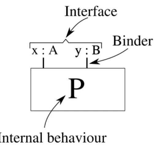
BlenXmodels biological components through boxes. A box is characterized by a process that describes the internal behaviour of the box and by a set of
binders that represent the capabilities of the box to interact with other boxes (see Figure 1). Each binder is associated with an identifier. A notion of affinity between binder identifiers define how boxes can interact. The quantitative value of the affinity provides also the stochastic information to drive the execution of programs. Binders with affine identifiers are also used to bind boxes together and originate complexes. The behaviour of a complex is defined by the boxes it is made up of.
Figure 1: We use box as abstractions of biological entities. Active sites, or domains, in a protein are represented as binders on the bio-process interface. Note the distinction between the interface, that makes possible interactions with other boxes, and the internal process, that defines the internal behaviour of the box.
The union between the set of free boxes (that do not belong to any complex) and the set of complexes is the set of molecules that populate the model. These molecules can perform monomolecular and bimolecular reactions. Monomolecu-lar reactions involve only one molecule as reactant; this molecule can, for exam-ple, expose a new binder, change the type of an existing binder or broke one of its bonds becoming two different molecules. Bimolecular reactions involve two molecules as reactant; in this case the two molecules can bind together forming a new molecule or communicate together changing their internal state.
BlenXalso supports events. An event is the composition of a condition and an action triggered only when the associated condition is satisfied. In particular there are four kinds of events: join, which substitutes two boxes with a single one; split, which substitutes a box with two boxes; new, which introduces a specified number of instances of a box; delete, which eliminates boxes. For simplicity we only consider join and split events.
A BlenX program is made up of two files: one defining the actions a system can perform and another one defining the affinities between binder identifiers. For more details and full examples we refer the reader to [5].
The BlenX approach mainly differs from other approaches like ODEs because these approaches do not consider the identity of the molecules. For example a reaction that form a complex from two molecules is expressed as A + B → C. This description may lead to possible misunderstanding: we cannot univocally
deduce that C is a complex composed of two molecules, we could think that A reacts with B,B is destroyed and A transforms into C.
Most process calculi implement instead the molecules A and B in such a way that they can interact together. Then when some instances of these molecule are run in a simulation they can form a complex. In this complex the two molecules keep their identity and looking at the C complex we can understand that it is composed of two different molecules.
The conceptual difference in the description of biological systems, makes it not immediate to translate directly process calculi programs into reaction based descriptions, and hence translate them into an SBML representation (www.sbml.org).
The aim of this paper is to present an algorithm to convert process calculi programs (in particular BlenX programs) into a list of reactions that can be exported in SBML format. Molecules implemented in BlenX, due to technical issues, perform some reactions with infinite rate. Before translating the program in SBML we can identify these reactions and in most of the cases remove them. In this way the exported model can be executed more efficiently and also by a bigger set of simulators; in fact some of them do not handle reactions with infinite rate.
In the next section we present the algorithm that performs the translation of a BlenX program into an optimized list of reactions; in the last section we present the conclusions of our work.
2
The Algorithm
The translation of a BlenX program into a list of chemical reactions extracts the molecules defined in the model and then deduces which reactions these molecules can perform. The procedure is iterated on the products of the reactions until it is reached a step that does not produce new species to be analysed. Stoichiometry is not taken into account; we always consider to have infinite copies of molecules. Reactions are then represented through a graph. This graph is analysed in order to reduce its size. Nodes that cannot be reached from the initial config-uration are pruned and some classes of immediate reactions are reduced. The reduced graph identifies a set of reactions that still represents the original BlenX program. These reactions are finally exported into a file in SBML format avail-able for further manipulations.
It is possible that the algorithm does not halt; for example, if a molecule can polymerise, the BlenX program can potentially generate a complex with an infinite number of components. Thus the algorithm needs an infinite number of steps to analyse all the molecules can be generated by the program. To solve this issue we can tell the algorithm to consider as possible reactants of a reaction only those complexes that are composed by no more then a prefixed number of molecules.
The algorithm does not halt too if a molecule can assume an infinite number of internal configurations. From a biological point of view it does not make any sense, but potentially in a BlenX program molecules with this behaviour can be defined. We do not handle this case given that it does not have any biological counterpart and thus we consider it as an error in the modelling strategy.
Summing up, the translation of BlenX programs into chemical reactions can be summarized in 3 main steps:
1. identification of molecules and reactions; 2. pruning of the reactions graph;
3. reduction of the immediate actions.
The next three sub-sections deal with the three items above.
2.1
Identification of molecules and reactions
FindReactions(BlenXProgram)1 Put in Boxes all the boxes defined in BlenXProgram 2 Put in Complexes all the complexes defined in BlenXProgram
3 Put in BimActions all the bimolecular action that the boxes can perform 4 for eachComplex in Complexes
5 doKnownComplexes[Complex ] = EmptyList()
6 while(IsEmpty(Boxes) == false and IsEmpty(BimActions) == false) 7 do while(IsEmpty(Boxes) == false)
8 Box= Boxes.pop()
9 MonoActions= GetMonoActions(Box )
10 CompNodeList= GetCompNodePairs(Complexes,Box ) 11 for eachMonoAction in MonoActions
12 doActionMap[Box ].Push(MonoAction) 13 for eachCompNode in CompNodeList
14 doReaction=ExMReaction(MonoAction,CompNode) 15 if (AddReaction(Reactions,Reaction) == True)
16 thenNewComp=UpdateLists(Reaction.Products,Boxes, Complexes,BimActions)
17 for eachComplex in NewComp
18 doKnownComplexes[Complex ]=
GetAnalysedActions(Complex ,ActionMap)
19 AllNewComp.Add(NewComp)
20 while(IsEmpty(BimActions) == false) 21 doBimAction= BimActions.Pop() 22 ActionMap[BimAction.e1] = BimAction 23 ActionMap[BimAction.E2] = BimAction
24 CompNodeList1= GetCompNodePairs(Complexes,BimAction.E1) 25 CompNodeList2= GetCompNodePairs(Complexes,BimAction.E2) 26 for eachCompNode1 in CompNodeList1
27 do for eachCompNode2 in CompNodeList2
28 doReaction= ExBReaction(BimAction,CompNode1 ,CompNode2 ) 29 if (AddReaction(Reactions,Reaction) == True) 30 thenNewComp= UpdateLists(Reaction.Products,Boxes, Complexes,BimActions)
31 for eachComplexin NewComp
32 doKnownComplexes[Complex ]=
GetAnalysedActions(Complex ,ActionMap)
33 AllNewComp.Add(NewComp)
34 CheckNewComp(AllNewComp,ActionMap,Boxes,Complexes,BimActions, KnownComplexes)
The procedure FindReactions collects all boxes (including those part of complexes) and complexes defined in BlenXProgram. In the next step all the bimolecular actions that can be performed by the boxes stored in Boxes are collected in the list BimActions. For each complex we store in the KnownComplexes hash map the list of all the actions that have the following properties:
• can be performed by some boxes that are components of the complex; • has been already analysed by the procedure FindReactions in previous
Given that the procedure has not yet started to analyse any action, all the complexes defined in the model are initially associated with an empty list.
After the initialization steps the main loop of the procedure starts. This loop continues until the list Boxes and the list BimActions are both empty. This loop is composed by two sub loops. The first loop (line 7) explores all the boxes and analyses which monomolecular reactions can be performed by these boxes. The second loop (line 20) analyses the bimolecular reactions.
We use the ActionMap indexed by boxes and that associates boxes to list of actions. An action associated with a box must satisfy the two following constraints:
• the box (or one of the two boxes in the case of a bimolecular action) involved in the action has to be the one the action is associated with; • this action has been already analysed in previous iteration or it is the
current action.
Consider the first loop. It extracts a box from the Boxes list and then, through the function GetMonoActions, gets all the monomolecular actions this box can perform.
Then the function GetCompNodePairs analyses all the complexes that contains the considered box. This function returns a list of pairs filled with the current complex and with a node that is a reference to a specific instance of the analysed box inside the complex. Therefore if a box is present twice in one complex the procedure will return two pairs, both of them with the same complex but with different nodes, one for each instance of the box inside the complex. If the box does not belong to any complex, the function returns a pair that has the box as node and Null as complex.
Each action in MonoActions, is inserted into the ActionMap, into the list as-sociated with the box currently analysed; then for each CompNode (a pair com-posed by a complex and a node) in the list CompNodeList the procedure ExM-Reaction is called. This procedure takes the complex specified in CompNode, applies the action MonoAction to the node specified in CompNode and returns Reaction, an object where the reactants, the products and the rate of the just examined reaction are stored.
After that the function AddReaction is called. This procedure updates the hash map Reactions, that associates reactions to a list of rates. These rates are the stochastic rates at which reactions take place into the BlenXProgram. Note that this is a list, because the same reaction can be performed in different way with different rates. Thus the AddReaction function adds the reaction only if it is not present in the map, otherwise it just add the new rate in to the list that is already associated with the reaction. The function returns True only if it adds the reaction to the map. In this case we call the function UpdateLists that analyses the products of Reaction, finds the complexes and the boxes produced by this reaction and generates the new bimolecular actions that the new boxes can perform. The function adds these new objects to the corresponding lists (Complexes, Boxes or BimActions). The new complexes are returned by the function are inserted in the KnownComplexes hash map together with the list of already analysed actions that the boxes they are made of can perform. This list of actions is created by the procedure GetAnalysedActions exploiting the ActionMap hash map.
Then the complexes stored in NewComp are inserted in AllNewComp. This list stores all the new complexes generated during the execution of the main procedure.
The second loop analyses bimolecular actions performing the same steps of the first loop. The only difference is that actions involve two boxes. This loop uses the same procedures and the same functions, the only exception be-ing ExBReaction used in place of ExMReaction. The former is used for bimolecular reactions the latter for monomolecular reactions.
After the two loops the CheckNewComp procedure (see pseudo-code be-low) is executed. It analyses the new complexes that have been created by the reactions identified in the current iteration of the main loop and applies to them all the reactions that have been already discovered and that are performed by an already analysed box they are made of.
CheckNewComp has a main loop that analyses all the complexes inside the CompToCheck list (instantiated by AllNewComp built in FindReactions). To find all the actions that must be applied to the current complex, the procedure exploits the infomration present in the KnonwComplexes hash map.
For each action there are two cases: the action can be monomolecular or bimolecular. In the first case the procedure gets the box that performs the action and looks for all the occurrences of the box inside the complex exploiting the function GetCompNodePairs. It returns the list of pairs CompNodeList: a pair for each occurrence of the box in Complex . From this point, each pair in CompNodeList is handled as in FindReactions at line 13.
The case of a bimolecular reaction involves two boxes, E1 and E2 , but these two boxes are not necessarily both part of the currently analysed plex. There are three different cases (lines 19-32): E1 is part of the com-plex and E2 is not, E2 is part of the comcom-plex and the E1 is not, and both boxes are part of the complex. In the first case we have to execute Action to analyse all the reactions that make react Complex with complexes which E2 belongs to, in the second case we have to do the same for reactions that make react Complex with complexes which E1 belongs to, in the third case we have to consider the union of the two previous cases. We create in this way, four lists of complex-node pairs: in the first case CompNodeList1 contains the pairs that represent the occurrences of E1 in Complex , CompNodeList2 contains the pairs that represent all the occurrences of E2 in the complexes present in Complexes and CompNodeList3 and CompNodeList4 are empty; in the second case the lists of CompNodeList1 contains the pairs that represent the occurrences of E2 in Complex , CompNodeList2 contains the pairs that represent all the occurrences of E1 in the complexes present in Complexes and CompNodeList3 and CompNodeList4 are empty; in the third case, that is the union of the previous ones, in CompNodeList1 and CompNodeList2 we have respectively the CompNodeList1 and CompNodeList2 of the first case and in CompNodeList3 and CompNodeList4 we have the CompNodeList1 and CompNodeList2 of the second case. At line 32 we delete the pairs that con-tain Complex from CompNodeList4 because to obcon-tain the union of the first and the second case we have to remove their intersection. The lists of pairs to be considered are treated as in FindReaction procedure at line 26.
After that all the complexes in CompToCheck have been analysed, the pro-cedure CheckNewComp is recursively called to analyse the new complexes generated during the execution of the current call.
CheckNewComp(CompToCheck ,ActionMap,Boxes,Complexes,BimActions,KnownComplexes) 1 for eachComplex in CompToCheck
2 doActions=KnownComplexes.actions 3 for eachAction in Actions
4 doTmpCompList.Push(Complex ) 5 ifActionis monomolecular
6 Box= Action.Box
7 thenCompNodeList=
8 GetCompNodePairs(TmpCompList,Box )
9 for eachCompNode in CompNodeList
10 doReaction=ExMReaction(Action,CompNode)
11 if (AddReaction(Reactions,Reaction) == True)
12 thenNewComp=UpdateLists(Reaction.Products,
Boxes,Complexes,BimActions)
13 for eachComplex in NewComp
14 doKnownComplexes[Complex ]=
GetAnalysedActions(Complex ,ActionMap)
15 AllNewComp.Add(NewComp)
16 ifActionis bimolecular
17 thenE1= action.E1
18 E2= action.E2
19 if IsInComplex(Complex ,E1 ) == True
andIsInComplex(Complex ,E2 ) == False
20 thenCompNodeList1=GetCompNodePairs(TmpCompList,E1 )
21 CompNodeList2=GetCompNodePairs(Complexes,E2 )
22 CompNodeList3=CompNodeList4 =EmptyList()
23 if IsInComplex(Complex ,E2 ) == True
andIsInComplex(Complex ,E1 ) == False
24 thenCompNodeList1=GetCompNodePairs(TmpCompList,E2 )
25 CompNodeList2=GetCompNodePairs(Complexes,E1 )
26 CompNodeList3=CompNodeList4 =EmptyList()
27 if IsInComplex(Complex ,E2 ) == True
andIsInComplex(Complex ,E1 ) == True
28 thenCompNodeList1=GetCompNodePairs(TmpCompList,E1 )
29 CompNodeList2=GetCompNodePairs(Complexes,E2 )
30 CompNodeList3=GetCompNodePairs(TmpCompList,E2 )
31 CompNodeList4=GetCompNodePairs(Complexes,E1 )
32 RemoveCompFromList(CompNodeList4 , Complex )
33 for eachCompNode1 in CompNodeList1
34 do for eachCompNode2 in CompNodeList2
35 Reaction=
ExBReaction(Action,CompNode1,CompNode2)
36 if (AddReaction(Reactions,Reaction) == True)
37 thenNewComp=UpdateLists(Reaction.Products,
Boxes,Complexes,BimActions)
38 for eachComplex in NewComp
39 doKnownComplexes[Complex ]=
GetAnalysedActions(Complex ,ActionMap)
40 AllNewComp.Add(NewComp)
41 for eachCompNode3 in CompNodeList3
42 do for eachCompNode4 in CompNodeList4
43 Reaction=
ExBReaction(Action,CompNode3,CompNode4)
44 if (AddReaction(Reactions,Reaction) == True)
45 thenNewComp=UpdateLists(Reaction.Products,
Boxes,Complexes,BimActions)
46 for eachComplex in NewComp
47 doKnownComplexes[Complex ]= GetAnalysedActions(Complex ,ActionMap) 48 AllNewComp.Add(NewComp) 49 TmpCompList.Clear() 50 CheckNewComp(AllNewComp,ActionMap,Boxes,Complexes,BimActions, KnownComplexes)
2.2
Pruning of the reactions graph
After the identification of the reactions, we check which of them can be removed because they can not be fired and which of them can be reduced because they have an infinite rate. To make these reductions easier, we represent the identified reactions in a graph made up of three kinds of elements: molecule nodes, multi
nodes and arcs.
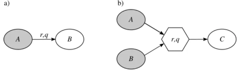
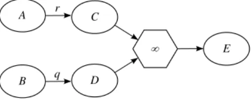
Molecule nodes represent molecules that are involved in the reactions and are labelled by unique names. Multi nodes represent reactions that involve more then one reactant or more then one product and are labelled with the list of rates at which the reaction can be executed. Arcs are used to represent monomolecular reactions and to connect molecules to multi node. In the first case they are associated with the list of rates the monomolecular reaction can be executed. Figure 2 shows two examples of how reactions are translated into graphs.
Figure 2: Two examples regarding the representation of reactions in the graph. Ellipses represent molecule nodes and hexagons represent multi nodes. a) Ex-ample of monomolecular reaction. It represents the reactions A → B that is associated with two rates: r and q. b) Example of bimolecular reaction. It represents the reaction A + B → C with rate r and q
Each molecule node has a flag stating whether it represents either a molecule that is defined in the BlenX program or a molecule that is the result of the execution of a reaction. Graphically (see Figure 2) we distinguish the nodes that are defined in the BlenX program by filling them in gray.
All the nodes can be reached starting from gray molecule nodes. We say that each node of the graph satisfy the reachability property. During the reduction of the graph, it happens that some nodes loose this property and we delete them because they cannot be created during a simulation.
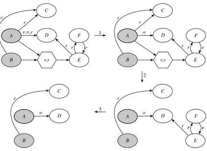
We delete reactions with finite rate that are in competition with other with infinite rate because they cannot be executed. This deletion is done in three steps. In the first step we just consider the list of rates associated with each reaction and for the lists that have an infinite rate we delete all the other rates (see step 1 in Figure 3).
In the second step we look for molecules that are involved as reactant in monomolecular reactions with infinite rate, and we delete all the reactions that take this molecule as a reactant.
In the third step we check all the products of the reactions that have been deleted, and, if they have lost the reachability property, they are deleted too. We also delete all the reactions where these products are involved as reactants. The reachability property is recursively verified until all the nodes of the graph are again reachable.
An example of the application of these three reduction steps is shown in Figure 3.
When we have finite rate reactions in competition with an immediate bi-molecular reaction we do not prune anything. This is because it could be that during a simulation one of the reactants of the bimolecular reaction is
Figure 3: Example of reduction of a graph through deletion of reactions that cannot be executed
not present. In this case the bimolecular reaction cannot be fired and the reac-tions with finite rate have to be considered. In Figure 4, for example, we have a bimolecular reaction with infinite rate that consumes A and B, and we cannot delete the finite rate reaction that transforms B in C because it can be triggered if during a simulation all the B molecules are consumed.
Figure 4: Example of graph where pruning is not applied.
2.3
Reduction of the immediate actions
The second reduction is the implosion of the reactions with infinite rate. Nodes that are involved exclusively in immediate reactions can be removed with some exception that will be discussed later; all the reactions with infinite rate that are removed can be replaced by non-immediate reactions between reactants and products of the deleted nodes.
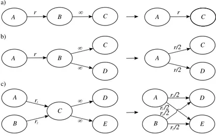
For the sake of clarity, we present the reduction of immediate reactions via some examples. In the first set of examples, shown in Figure 5, we report cases that involve just molecule nodes. In Figure 5.a we consider two consecutive reactions where the second one has infinite rate. In this situation A is trans-formed in B with rate r; B immediately reacts and it is transtrans-formed in C. It is easy to realize that in this example the molecule B is transient: every time it
appears it is immediately transformed into another molecule. Thus it is possible to eliminate the molecule B from the graph and make A directly transforms in C with rate r.
In Figure 5.b we have A that reacts and changes in B with rate r, than with equal probability B immediately transforms in C or D. Also in this case it is easy to realize that B is transient and can be deleted from the graph. The difference with the previous case is that now it is important to adjust the rate in order to keep the same probability to move from A to C and from A to D. The procedure to follow consists in adding to A all the sons of B. The rates of these reactions is given by the rate r divided by the original number of sons of B.
With the last example of Figure 5 we introduce the general procedure to reduce transient nodes that have exclusively molecule node as reactants and products. In this case the node to eliminate is C:
DeleteMonoMono(Graph, T )
1 n = number of reactions that involves T as reactant in Graph 2 for each molecule node X in Graph involved in reactions X → T
3 do for each molecule node Y in Graph involved in reactions T → Y 4 doadd to Graph reaction X → Y
5 set rate of X → Y with rate of X → T divided by n 6 Delete(Graph, T )
To delete the transient node T we use the function Delete that we define in the following pseudo code:
Delete(Graph, T )
1 for each multi node X involved in reactions T → X 2 doremove from Graph node X
3 for each multi node X involved in reactions X → T 4 doremove from Graph node X
5 remove from Graph node T
In this procedure we delete also all the multi nodes connected to T . Consider the deletion of transient molecule nodes that have exclusively molecule nodes as reactants and multi nodes as products.
In Figure 6.a we show the case where B has one molecule node as reactant and one multi node as product. In this example A changes in B with rate r and B immediately divides and generates two molecules: C and D. Given that B is transient we can delete it and make A directly divide in C and D. The rate of this reaction is r.
In the example in Figure 6.b the transient node C has two molecule nodes as reactants and one multi node as product. The two reactants, A and B, can transforms both in C; then C immediately divides in D and E.
After the deletion of C, we want that its reactants, A and B, with two distinct reactions, directly divide in D and E. To achieve this goal, as first step, we add a multi node node to every original reactant of C. Then the old rates of these reactants are associated with the new multi nodes, and we add to each multi node the products of the multi node associated with the infinite rate. As last step we delete C and its associated multi node with the infinite rate.
Figure 5: Examples of deletion of molecule nodes that have exclusively molecule nodes as reactant and products
Figure 6: Examples of deletion of molecule nodes that have molecule nodes as reactant and multi nodes as products
Figure 7: Example of deletion of molecule nodes that have molecule nodes as reactants and multi nodes as products.
Consider the example shown in Figure 7 where the transient node has two molecule nodes as reactants and two multi nodes as products. This case is very similar to the previous one; the duplication of the multi nodes is repeated for each products of C and we perform the adjustment of the rates as we did in the example shown in Figure 3.c. The general procedure used to delete transient nodes that have molecule nodes as reactants and multi nodes as products is the following:
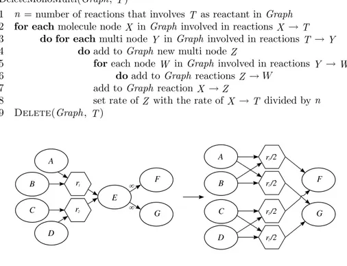
DeleteMonoMulti(Graph, T )
1 n = number of reactions that involves T as reactant in Graph 2 for each molecule node X in Graph involved in reactions X → T 3 do for each multi node Y in Graph involved in reactions T → Y 4 doadd to Graph new multi node Z
5 foreach node W in Graph involved in reactions Y → W 6 doadd to Graph reactions Z → W
7 add to Graph reaction X → Z
8 set rate of Z with the rate of X → T divided by n 9 Delete(Graph, T )
Figure 8: Example of deletion of molecule node that have multi nodes as reac-tants and molecules nodes as products.
Consider the example shown in Figure 8 where the transient node E has multi nodes as reactants and molecule nodes as products. This case is similar to the one just analysed so we directly propose the general pseudo code to handle this case:
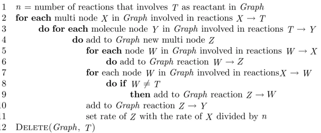
DeleteMultiMono(Graph, T )
1 n = number of reactions that involves T as reactant in Graph 2 for each multi node X in Graph involved in reactions X → T
3 do for eachmolecule node Y in Graph involved in reactions T → Y 4 doadd to Graph new multi node Z
5 for eachnode W in Graph involved in reactions W → X 6 doadd to Graph reaction W → Z
7 foreach node W in Graph involved in reactionsX → W
8 do if W 6= T
9 thenadd to Graph reaction Z → W 10 add to Graph reaction Z → Y
11 set rate of Z with the rate of X divided by n 12 Delete(Graph, T )
The last case we consider is the deletion of a transient node that has multi nodes as reactants and multi nodes as products. An example is shown in Figure 9 where the node E is transient and can be deleted.
Also in this case we only present the pseudo code that perform the reduction of interest:
DeleteMultiMulti(Graph, T )
1 n = number of reactions that involves T as reactant in Graph 2 for each multi node X in Graph involved in reactions X → T
3 do for eachmulti node Y in Graph involved in reactions T → Y 4 doadd to Graph new multi node Z
5 for eachnode W in Graph involved in reactions W → X 6 doadd to Graph reaction W → Z
7 foreach node W in Graph involved in reactionsX → W
8 do if W 6= T
9 thenadd to Graph reaction Z → W
10 for eachnode W in Graph involved in reactionsY → W 11 doadd to Graph reaction Z → W
12 set rate of Z with the rate of X divided by n 13 Delete(Graph, T )
Figure 9: Example of deletion of molecule node that have multi nodes as reac-tants and multi nodes as products.
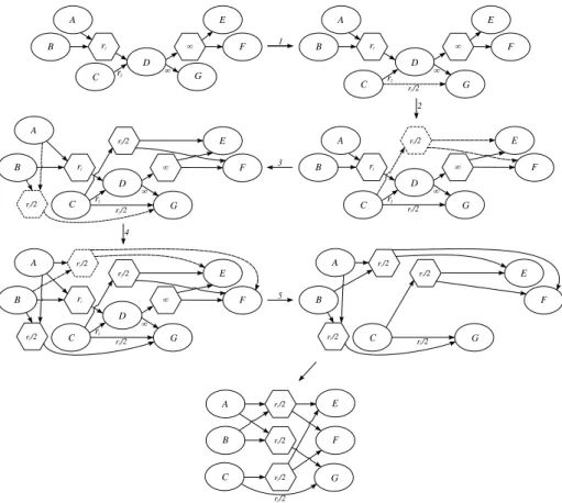
Now we examine a general example. In Figure 10 we have a transient node with a multi node and a molecule node as reactants and a multi node and a
molecule node as products. To delete this node we apply consecutively all the procedure we presented. We mark the used procedures with an asterisk because they differ from the previous definition: in each procedure marked with the asterisk the procedure that deletes the transient node and its connected multi nodes is not called (last line of their pseudo-code). We perform the deletion of these nodes at the end of the procedure only once.
DeleteNode(Graph,T ) 1 DeleteMonoMono*(Graph,T ) 2 DeleteMonoMulti*(Graph,T ) 3 DeleteMultiMono*(Graph,T ) 4 DeleteMultiMulti*(Graph,T ) 5 Delete(Graph, T )
In Figure 10 we show the application of the procedure DeleteNode on a specific example. The numbers on the arrows indicate which line of code is executed in the transition. In the last step we only adjust the positions of the nodes in order to obtain a clearer picture.
Figure 10: Example of deletion of molecule node that have a molecule node and a multi node as reactants and molecule node and a multi node as products.
immediate actions, now we present an example where we cannot. In Figure 11 we have two molecules, C and D, that seem to be transient because there is a bimolecular reaction that with infinite rate consumes them. Unfortunately the molecules are not transient because if there is not any C molecule in the system, D molecules are not immediately transformed. This make impossible to apply the previous solution to this example. So in this case we do not reduce the action with infinite rate.
Figure 11: Example of immediate reaction that we cannot reduce.
3
Conclusion
In this paper we presented an algorithm to convert a BlenX program into a list of reactions. A BlenX program leads to the execution of some immediate reactions (reactions with infinite rate) that we can reduce through our algorithm. We export the optimized model into an SBML file that can be imported by simulators that support this format like Copasi [7], Dizzy [16] and Stochkit [8]. The optimization that we perform on BlenX programs makes possible to model biological systems without consider performance issues. A program can be written in the most intuitive form, introducing all the necessary immediate reactions because they are successively removed by the described algorithm.
Acknowledgements. We thank L. Dematt´e and A. Romanel for useful comments and discussions.
References
[1] Cardelli, L., Brane calculi., in: CMSB, 2004, pp. 257–278.
[2] Chiaverini, M. and V. Danos, “A core modeling language for the working molecular biologist,” Lecture Notes in Computer Science 2602, Springer, 2003 .
[3] Degano, P., D. Prandi, C. Priami and P. Quaglia, Beta-binders for Biolog-ical Quantitative Experiments, in: Proc. of the 4th International Workshop on Quantitative Aspects of Programming Languages (QAPL 2006), ENTCS 164(2006), pp. 101–117.
[4] Dematt´e, L., C. Priami and A. Romanel, BetaWB: modelling and simu-lating biological processes, in: 2007 Summer Simulation Multiconference, 2007, pp. 777–784.
[5] Dematt´e, L., C. Priami and A. Romanel, The BlenX language: a tutorial, in: M. Bernardo, P. Degano and G. Zavattaro, editors, Formal Methods for Computational Systems Biology, Lecture Notes in Computer Science (2008), to appear.
[6] Hoare, C., Communicating sequential processes, Comm. ACM 21 (1978), pp. 666–677.
[7] Hoops, S., S. Sahle, R. Gauges, C. Lee, J. Pahle, N. Simus, M. Singhal, L. Xu, P. Mendes and U. Kummer, Copasi - a complex pathway simulator., Bioinformatics 22 (2006), pp. 3067–3074.
[8] Li, H., Y. Cao, L. R. Petzold and D. T. Gillespie, Algorithms and software for stochastic simulation of biochemical reacting systems, Biotechnol. Prog. (2007).
URL http://dx.doi.org/10.1021%2Fbp070255h
[9] Milner, R., “Communication and Concurrency,” Prentice-Hall, Inc., 1989. [10] Phillips, A. and L. Cardelli, A correct abstract machine for the stochastic
pi-calculus, in: Bioconcur’04 (2004).
[11] Prandi, D., C. Priami and P. Quaglia, Communicating by compatibility, Journal of Logic and Algebraic Programming 75 (2008), pp. 161–180. [12] Priami, C., The stochastic π-calculus, The Computer Journal (1995),
pp. 578–589.
[13] Priami, C. and P. Quaglia, Beta binders for biological interactions, in: CMSB, 2004, pp. 20–33.
[14] Priami, C. and P. Quaglia, Operational patterns in beta-binders, T. Comp. Sys. Biology 1 (2005), pp. 50–65.
[15] Priami, C., A. Regev, E. Shapiro and W. Silvermann, Application of a stochastic name-passing calculus to representation and simulation of molec-ular processes, Inf. Process. Lett. 80 (2001), pp. 25–31.
[16] Ramsey, S., D. Orrell and H. Bolouri, Dizzy: Stochastic simulation of large-scale genetic regulatory networks, J. Bioinformatics and Computational Bi-ology 3 (2005), pp. 415–436.