Department of Business and Management
Chair of Advanced Corporate Finance
The profitability of Capital Structure Arbitrage from 2015 to
2017: evidence on volatility estimator and companies’ leverage
SUPERVISOR
Prof. Oriani Raffaele
CANDIDATE Marini Marco 675781
CO-SUPERVISOR
Prof. Curcio Domenico
Contents
1 Introduction ... 3
2 Capital structure and debt riskiness ... 6
2.1 Introduction ... 6
2.2 Capital Structure Theory ... 7
2.2.1 The irrelevance of capital structure ... 7
2.2.2 The Trade-off Theory ... 10
2.2.3 The Pecking Order Theory ... 11
2.3 The evolution of structural models for debt pricing ... 13
2.3.1 Merton Model ... 14
2.3.2 Black and Cox Model ... 18
2.3.3 Geske Model ... 21
2.3.4 Kim, Ramaswamy and Sundaresan Model ... 21
2.3.5 Longstaff and Schwartz Model ... 23
2.3.6 Leland and Toft Model ... 24
2.3.7 Zhou Model ... 25
2.3.8 Briys and Varenne Model ... 27
2.3.9 Fan and Sundaresan Model ... 29
2.3.10 CreditGrades Model ... 30
2.3.11 Cremers, Driessen and Maenhout Model ... 34
2.3.12 Zhang, Zhou and Zhu Model ... 34
2.3.13 Reduced form models ... 35
2.4 Conclusion ... 41
3 Capital Structure Arbitrage ... 42
3.1 Introduction ... 42
3.2 Strategy description and historical profitability ... 44
3.2.1 Capital Structure Arbitrage Literature Review ... 45
3.2.2 Strategy Implementation ... 49
3.2.3 Main findings on Capital Structure Arbitrage ... 57
3.3 The CreditGrades model in more depth ... 62
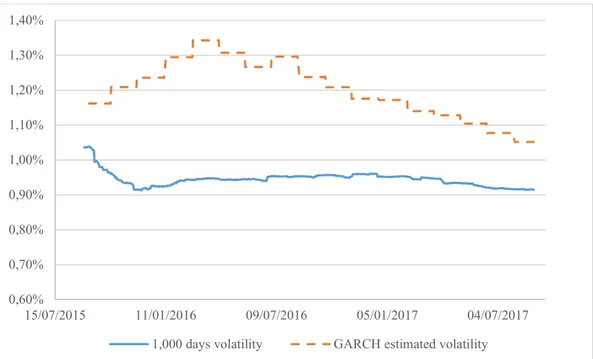
3.4 A GARCH approach to calibrate equity volatility ... 65
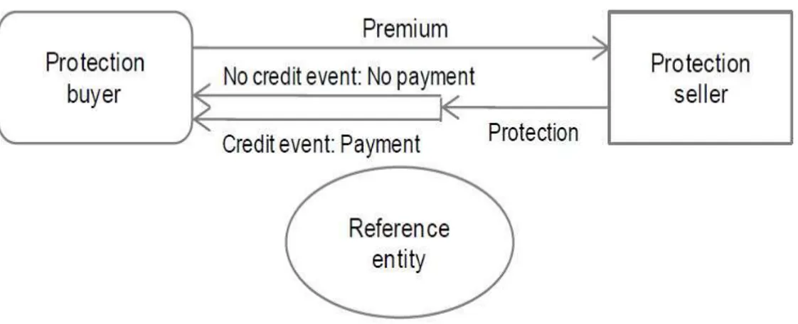
3.5 Credit default swaps ... 68
3.5.1 Core elements of a CDS contract ... 68
3.5.3 Settlement ... 71
3.6 Conclusion ... 74
4 Capital Structure Arbitrage profitability and the effects of GARCH ... 76
4.1 Introduction ... 76
4.2 Data collection ... 77
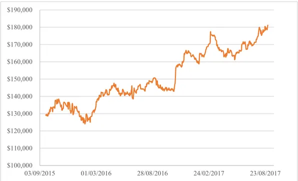
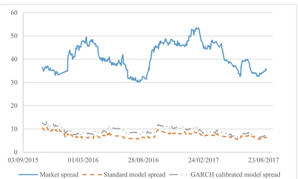
4.3 Strategy implementation: the case of Berkshire Hathaway ... 79
4.4 General results for individual trades ... 86
4.5 Observations on the role of leverage ... 95
4.6 Conclusion ... 100
5 Conclusion ... 102
3
1
Introduction
The topic of this thesis will be the investment strategy known as Capital Structure Arbitrage and the predictive models that serve to implement this strategy.
Capital Structure Arbitrage prescribes to trade one security against another security issued by the same firm. A common way to implement the arbitrage is to trade the debt against the equity of a given firm. Generally, it is implemented trading stocks and CDSs.
The willingness to deepen the knowledge on this arbitrage strategy comes from the scarcity of academic research on the subject and the will to deepen the knowledge on models developed to estimate default probability. In fact, how it will be later clearer, a correct implementation of the Capital Structure Arbitrage requires, as input, a correct and timely estimation of default probability of companies through time. The success of Capital Structure Arbitrage is therefore strictly linked to the effectiveness of these models.
In particular, this work will enquiry if Capital Structure Arbitrage is still a profitable investment strategy and if there is, eventually, room for improvement in strategy execution. The last found paper written on the subject, in fact, dates back to 2014 and it concludes that the profitability of the strategy seems to be linked to specific time periods.1 Moreover, the Capital Structure Arbitrage profitability could have
been explained, in past years, by a low liquidity of credit default swap (CDS) market. It is therefore of interest to understand if the development of derivatives trade during last years affected the profitability of the strategy. The strategy, in fact, earns from the mispricing of credit default swaps. Therefore, an increase in CDSs liquidity could have led to a higher market efficiency in pricing these derivative products and no profit left for arbitrageurs. This vision is shared by Cserna & Imbierowicz (2008), that found that the average returns of the strategy appears to decline over time, and that this phenomenon could be explained by an increased efficiency of the credit default swap market.
1 Wojtowicz, M. (2014). Capital Structure Arbitrage Revisited. Duisenberg School of Finance - Tinbergen Institute Discussion Paper; Working Paper.
4
At the same time, several authors remarked the importance of model’s parameters setting to have acceptable CDS spread previsions.2 In particular, the parameter that
has mostly been subject of study is the equity volatility.3
I will start the discussion of the topic with a literature review on debt riskiness and capital structure decisions. The arbitrage strategy under analysis, in fact, feeds on the inconsistent valuation of debt and equity of the same entity. A review of the more common theories on capital structure composition is therefore proposed. Those are, in fact, theories that try to explain the relation between the value of the firm as a whole and the value of the single parts of its capital structure, that is equity and debt.
Hence, an historical digression on structural models is reported. Starting from the model proposed by Merton in 1974, the other structural models developed on it are analyzed. Structural models are models developed to formally link firm’s asset value with debt and equity value. The improvements of new models are highlighted and a synoptic table is proposed.
Then, the features of Capital Structure Arbitrage are analyzed. The investment strategy will be dissected and the various approach reported in academia will be compared, as well as the result obtained by various authors.
Since one of the main point of discussion on Capital Structure Arbitrage is represented by the correct way to calibrate the equity volatility in the structural model chosen to implement the arbitrage, an innovative approach to volatility calibration will be proposed.
Finally, the results of a simulation of the analyzed strategy is proposed. The simulation is performed through a back-testing of the arbitrage in the period from August 2015 to August 2017.
The aim of the strategy back-testing is to understand if Capital Structure Arbitrage is still able to produce attractive returns and if the introduction of GARCH as volatility estimator can have a positive effect on strategy effectiveness.
2 See, for instance, Bajlum, C. & Larsen, P. T. (2008). Capital Structure Arbitrage: Model Choice and Volatility Calibration. Copenhagen Business School, Department of Finance, Working Papers. 3 See Bajlum & Larsen (2008), Avino, D. & Lazar, E. (2013). Rethinking Capital Structure Arbitrage: A Price Discovery Perspective. MPRA Paper, University Library of Munich and Wojtowicz (2014).
5
Interestingly, the strategy simulation shed light on a feature of structural models used that was not mentioned in no one of previous works on the matter. In particular, the role of leverage seems to play a fundamental role on the ability of the model to predict market spreads. A possible explanation of the phenomenon is proposed.
6
2
Capital structure and debt riskiness
2.1 Introduction
This chapter will illustrate the determinants of the riskiness of corporate debt and the effects of capital structure composition on companies’ market value.
The implementation of an arbitrage on firms’ capital structure requires, in fact, that debt and equity are not priced consistently. Debt and equity are the two components of the capital structure of every firm and their characteristics, in terms of riskiness and value, are linked to the same entity, that is the assets of the firm.
The effect of different shapes of capital structure on assets’ value has raised debates in academy. Different theories arose, from the famous irrelevance of capital structure, firstly theorized by Modigliani and Miller (1958) to the more recent Pecking Order Theory. Anyway, it is undeniable that the value of firm’s debt and equity are, in some way, affected by the firm’s capital structure and are both derivative of the firm’s asset value.
Therefore, this chapter will, first of all, present the more relevant theories produced on the topic of capital structure.
Successively, the more relevant literature on structural models will be reported. Structural models are models developed to formally link firm’s asset value and the value of its capital structure components. Structural models make use of theories on capital structure and go beyond in the determination of the mechanism that links the two side of the “market value balance sheet”. Most of the early structural models, in fact, stately relies on the theory of Modigliani and Miller (1958). The usefulness of these models to the purposes of this thesis relies on the fact that structural models can predict from market variables the probability of default of a firm.
The purpose of this chapter is therefore to introduce and explain the relevant literature on capital structure theory and the development, through the years, of models for debt pricing.
7
2.2 Capital Structure Theory
The arbitrage strategy I am going to analyze in this work has its reason in the mispricing of one part of the capital structure respect to another. According to Pedersen (2015), this trade is based on the idea that all claims to the firm are derivatives of the firm value and if these are not priced consistently, arbitrage opportunities arise. Therefore, a discussion on the more common theories on capital structure composition appear useful, since debt and equity valuation start from the comprehension of their interrelations with company’s asset value.
Many research papers on the effects of capital structure composition on the firm’s value and the determination of an optimal leverage ratio has been produced during last decades. No one produced a definitive answer. On the contrary, different theories arose, testifying how the capital structure valuation of firms is still a discussed topic. The theories on the effect of capital structure on firm’s value and the resultant effect on the valuation of capital structure’s components are an element to take under consideration in implementing an arbitrage strategy that exploits the pricing of debt and equity. These theories, in fact, give the basis to understand the elements affecting debt and equity pricing.
2.2.1 The irrelevance of capital structure
The most popular seminal work on capital structure composition is the paper from Modigliani and Miller of 1958. They claim that the capital structure is not relevant in determining the value of a firm. In their work, the author approaches the discussion on capital structure under the hypothesis of uncertain outcomes of firm’s operations. Their theory relies on the assumption of perfect capital markets. This assumption entails a range of features on the environment of their research: particularly relevant is the absence of frictions and taxes in the market. The starting point of this theory is that the value of a firm comes solely from the expected return on its assets. In their proposition I, in fact, the authors say that the average cost of capital of any firm is completely independent of its capital structure and it is equal to the capitalization rate of a pure equity stream of its class.4 Hence, the average
4 Miller, M. & Modigliani, F. (1958). The Cost of Capital, Corporation Finance and the Theory of Investment. The American Economic Review, 48(3), 261-297.
8
cost of capital of a firm is derived by the expected returns of the firm’s asset and by the volatility of these returns. The cost of equity and debt is therefore direct function of the expected return on the assets. Value of equity and of debt are given by the level of leverage of the firm, and their sum equals the value of the firm’s assets. This implies that for higher level of debt, the equity becomes riskier and therefore the required return on it increases but its weight on the average cost of capital decreases, leaving the expected return on assets constant. Similarly, debt becomes more risky for higher level of indebtedness, but in a different way respect to the equity. While the cost of equity rises as a compensation for the higher volatility of its return, debt’s price increases when the variability of firm’s return produces the risk of default on debt. High level of debt, in fact, entails the real possibility of default on debt, making it more similar to equity. As the leverage increase, the cost of debt will therefore increase to reach, in the extreme case, the cost of risky equity. The dynamic of debt’s cost for different level of leverage is a direct consequence of the variability of the streams of revenues of the firm.
Anyway, the total cost of capital for the firm is its average cost of capital and it is determined exclusively by the expected return of the firm’s assets, no matter how the capital structure is composed.
The relation among the return on asset and the cost of debt and equity, according to the theory from Modigliani and Miller, is expressed in the proposition II by the following equation:
𝑟 =𝐸
𝑉 𝑟 + 𝐷 𝑉 𝑟
where 𝑟 is the expected return on assets, 𝑟 is the expected return on equity and 𝑟 the required return on debt. E, D and V are, respectively, the market value of equity, debt and the whole firm.
The previous equation can be rearranged to solve for 𝑟 as
𝑟 = 𝑟 + 𝐷
𝐸 (𝑟 − 𝑟 )
that is, the expected yield of a share is equal to the appropriate capitalization rate 𝑟 of a pure equity stream plus a premium for the financial risk coming from the
9
level of leverage and the spread between 𝑟 and 𝑟 .5 If the firm were financed solely
through equity, in fact, 𝑟 would equal 𝑟 . Introducing debt, the return on equity requires a premium for the additional risk.
If we refer to the proposition II’s equation in terms of the beta of each segment of the capital structure, we would have that
𝛽 =𝐸
𝑉 𝛽 + 𝐷 𝑉 𝛽 Given that the beta of stock i can be expressed as
𝛽 =𝑐𝑜𝑣(𝑟 , 𝑟 ) 𝑣𝑎𝑟(𝑟 )
and the covariance between stock i returns and market returns as 𝑐𝑜𝑣(𝑟 , 𝑟 ) = 𝜎 𝜎 𝜌,
where 𝑟 is the return of stock i, 𝑟 is the return of market portfolio and 𝜌, is the
correlation among 𝑟 and 𝑟 , the equation of 𝛽 can be rewritten as 𝑐𝑜𝑣(𝑟 , 𝑟 ) 𝑣𝑎𝑟(𝑟 ) = 𝐸 𝑉 𝑐𝑜𝑣(𝑟 , 𝑟 ) 𝑣𝑎𝑟(𝑟 ) + 𝐷 𝑉 𝑐𝑜𝑣(𝑟 , 𝑟 ) 𝑣𝑎𝑟(𝑟 )
If we express the covariance as the product of the volatility of the two variables and their correlation, the above equation becomes
𝜌 , 𝜎 𝜎 =𝐸
𝑉 𝜌 , 𝜎 𝜎 + 𝐷
𝑉 𝜌 , 𝜎 𝜎 Rearranging and solving for 𝜎 and 𝜎 we have
𝜎 =𝜌 , 𝜌 , 𝜎 + 𝐷 𝐸 𝜌 , 𝜌 , 𝜎 − 𝜌 , 𝜌 , 𝜎 𝜎 = 𝜌 , 𝜌 , 𝜎 + 𝐸 𝐷 𝜌 , 𝜌 , 𝜎 − 𝜌 , 𝜌 , 𝜎
Looking at the theory of Modigliani and Miller by this perspective highlights the link between the volatility of the assets’ return, the volatility of debt and equity and the level of leverage of a firm. Both the volatility of debt and equity are function of asset’s volatility and capital structure.
5 Ibid.
10
Since the asset of a firm are not traded, the parameters 𝜎 and 𝑟 are not variables that can be observed in the market. The prediction of theoretical value for 𝑟 and 𝑟 therefore required the creation of sophisticated models, that will be debated later.
2.2.2 The Trade-off Theory
A theory, that evolves from the theory of Modigliani and Miller, is the Trade-off theory. This theory maintains the basic assumptions made by Modigliani and Miller but furthermore takes under consideration the costs of financial distress. Under perfect capital market’s assumptions, in fact, the default would simply produce the passage of the firm from the shareholders to the debtholders without affecting the total value available to investors as a whole. Debtholders are remunerated for the risk of suffering the cost deriving from a potential poor economic performance of the firm and the consequent loss in value. Under the Modigliani and Miller model the risk of bankruptcy is not a disadvantage of leverage.6 In the real world, the
financial distress and the default implicate costs for the firm. A firm that is no longer able to repay its debt will likely face the costs of debt restructuring, the cost of lawyers, problems with supplier and the loss of corporate going concern, just to report someone. This implies that a higher level of debt, and hence a higher probability of distress, will affect negatively the ability of a firm to raise new debt and will increase its cost of capital.
The trade-off theory says that the value of a levered firm is equal to its unlevered value plus the present value of the tax benefit minus the present value of the distress costs. This theory says that exists an optimal capital structure that maximize the value levered of a firm, minimizing its cost of capital.
The equation of the required return on assets can be easily modified to consider the effects of taxes and costs of distress. Taxes are in fact a benefit of leverage: a higher level of debt produce higher interest expenses that will reduce the taxable income. On the other hand, debt entails the risk of default. The equation of the required return on asset under the hypothesis of taxes and distress cost will hence appear to be
11
𝑟 = 𝐸
𝑉 𝑟 + 𝐷
𝑉 𝑟 (1 − 𝜏) + ( 𝑃𝐷 ∙ 𝐷𝐶)
where (1 − 𝜏) and ( 𝑃𝐷 ∙ 𝐷𝐶) are corrective factors that take into consideration taxes and distress costs: 𝜏 is the tax rate for the firm while ( 𝑃𝐷 ∙ 𝐷𝐶) is the probability of default given that level of leverage times the cost of default. It is important to note that while 𝜏 is a fixed percentage, ( 𝑃𝐷 ∙ 𝐷𝐶) is a function of the level of indebtedness and hence the probability to suffer from financial distress. By the equation above follows that the arbitrageur should take into account, when trying to price fairly debt and equity, the effect of taxes and the probability of financial distress.
2.2.3 The Pecking Order Theory
Another diffused theory regarding capital structure is the Pecking Order Theory. This theory does not try to individuate an ideal level of indebtedness, but rather it provides the order the firm will use in raising funds. According to the pecking order theory a firm will firstly use internal funds, then debt, finally equity. The reasons behind this theory are in the asymmetric information and in the opportunistic behavior of management that debt incentivizes.
The presented theories all try to explain the effect of capital structure’s choices on the value of a firm and of the components of its capital structure. The theories presented show how the capital structure influences the value of the company and how it is a determinant of the value of single segments of the structure.
Of higher interest for this work are those theories that try to formally link the value of the firm to the value of its capital structure components. The paper from Modigliani and Miller started to approach the problem by this standpoint and gave rise to further development of their theory.
Fundamental both in the Modigliani and Miller theory and in the Trade-off theory is to consider the expected return on equity and on debt derivatives of the expected return on the total assets. The value of debt and equity is simply given by the target leverage ratio of the firm. Fluctuations in the value of asset are followed by the rebalancing of the capital structure towards the desired level of leverage and the valuation of debt is obtained by multiplying asset value respectively for the
12
percentage of debt on the total asset. Similarly is obtained the valuation of equity value. But if we consider the problem by the perspective illustrated by the Trade-off theory the valuation of equity and debt is not so straightforward as it is under the assumption of Modigliani and Miller. The level of leverage, in fact, has an impact on the value of total asset. The leverage produce both an increase and a decrease in asset value. The increase is due to the saving in tax that debt allows: interests paid on debt are deductible from the taxable income. The decrease is a consequence of the higher likelihood of default that leverage produces.
In both the case, anyway, the practical link between the asset and the capital structure remains to be solved, since, as previously noted, the firm’s assets is not something exchanged in the market.
Since that if the firm is financed only by equity, the problem would not exist, the role of debt has been subjected to an intense work of research. Many models have been developed, aiming to estimate the probability that a firm will suffer from financial distress and incorporating this information in debt pricing. Different theories raised, aiming at produce models able to embody the relevant factors that affects the pricing of debt on the market.
In the next section, I will present the more relevant structural models for the pricing of debt. These models play an important role in the implementation of the capital structure arbitrage, because represent the term of comparison of the observed values in the market with their theoretical values. The use of these models hence allows to have a signal of market’s mispricing and the rise of possibility of arbitrage. The ability of structural models to obtain a measure of the probability of default for a firm allows to understand if the credit default swaps on a given security are fairly priced. A broader description of the reasons for the use of CDSs in the implementation of capital structure arbitrage is reported in next chapters.
13
2.3 The evolution of structural models for debt pricing
The need to have a clear understanding and a theoretical term of comparison of the implication of a given level of leverage on the value of asset and consequently on the value of the component of its capital structure has been addressed creating models able to include the expectations that a firm will suffer from financial distress.
The prediction of parameters such as the probability of default and credit spread on corporate bonds is important for the purposes of this work because are these parameters that signal the presence of arbitrage opportunities. Typically, the implementation of the Capital Structure Arbitrage looks at the pricing of debt and at the implied probability of default and of recovery of a given firm perceived from the market and compare these values with the theoretical values that the model suggests.7
There are two basic approaches to modeling corporate default risk. The first one is the structural model approach, pioneered by Black and Scholes (1973) and Merton (1974) and extended then by various authors, such as Black and Cox (1976), Geske (1977), Kim, Ramaswamy & Sundaresan (1993), Longstaf & Schwartz (1995) Leland & Toft (1996) and Zhou (1997). The structural pricing models imply the definition of firm’s value evolution as a variable observable by investors.8 The firm
defaults when its market value falls below an exogenously determined threshold, that in several models has been identified with the value of firm’s debt.
Another fundamental feature of the models proposed by Merton in 1974, and common to most of its subsequent evolutions, is the assumptions that firm’s value follows a diffusion process.
The second approach to default modeling is the reduced form approach. Under this approach, adopted, among the others, by Duffie & Singleton (1994), Jarrow, Lando, & Turnbul (1994), Jarrow & Turnbull (1995) and Madan & Unal (1994), the
7 See, for instance, Bajlum & Larsen (2007), Avino & Lazar (2013), Yu, F. (2006). How profitable is capital structure arbitrage? Financial Analysts Journal, 62(5), 47-62 and Cserna, B. &
Imbierowicz, B (2008). How Efficient are Credit Default Swap Markets? An Empirical Study of Capital Structure Arbitrage Based on Structural Pricing Models. 21st Australasian Finance and Banking Conference.
8 Zhou, C. (1997). A Jump-Diffusion Approach to Modeling Credit Risk and Valuing Defaultable Securities.
14
relation between firm’s value and default is not modeled in a structural way. This means that default could happen as a “surprise”, being its happening not explicitly linked to firm’s value. Default is treated in reduced form models as a random variable.
2.3.1 Merton Model
The work of research on structural models started after the publication of the paper from Merton (1974), that give further application to Black and Scholes (1973). Black, Scholes and Merton, in fact, introduced a contingent-claims approach to valuing corporate debt using option pricing theory.9 In their model, the value of a
firm’s debt is contingent on the market value of its assets. In their paper, Black and Scholes (1973) propose a model for the pricing of European options, based on no-arbitrage principle, that can be extended to the valuation of corporate liabilities. The authors claim that, since all corporate liabilities can be viewed as a combination of options, the formula proposed for their pricing is also applicable to corporate liabilities. Further, their model could also be useful in deriving the discount to apply to corporate bonds because of the possibility of default. Their reasoning starts observing how, under certain assumptions, the value of common shares can be viewed as an option on the firm’s assets. 10 Thus, the value of the common stocks
is given by the formula Black and Scholes derived for the pricing of call options, where the strike price c is equal to the book value of the firm’s debt, the variance of the underlying 𝑣 is the variance rate of return on firm’s asset and the underlying’s price 𝜘 is the total value of company assets. According to Modigliani and Miller proposition I, then they say that the value of the bonds will simply be the value of assets 𝜘 minus the value of the option on company’s assets, that individuate the value of the equity. In this way, the authors propose the use of their option pricing formula to price the corporate debt, taking into account the volatility
9 Bohn, J. R. (2000). A Survey of Contingent‐Claims Approaches to Risky Debt Valuation. The Journal of Risk Finance, 1(3), 53-70.
10 In their example, the authors consider a firm with common stocks and bonds outstanding. The bonds are pure discount bonds with no coupon payments, giving the holder the right to a fix amount of money at maturity. The bonds contain no restrictions on the company, except that the company cannot pay any dividends until the bonds are paid off. Finally, the company plans to sell all its asset at bonds’ maturity, pay off the bond holders, if possible, and pay a liquidating dividend to the stock holders with any remaining money.
15
of company’s assets and the linked probability of default. The authors propose also their model to figure out the discount that should be applied to bonds, due to the existence of default risk. The proposed procedure to individuate bond’s spread consists on subtracting the value of the bonds, given by 𝜘 minus the value of the option on company’ s assets, from the value they would have if there were no default risk.
Merton (1974) studies further the pricing of corporate debt, developing, along the Black-Scholes lines, a basic equation for the pricing of corporate debt. To develop his model, Merton makes a series of assumptions. In particular, the dynamics through time for the value of the firm V is described by the following stochastic differential equation
𝑑𝑉 = (𝛼𝑉 − 𝐶)𝑑𝑡 + 𝜎 𝑉𝑑𝑧
where 𝑎 is the instantaneous expected rate of return on the firm per unit of time, 𝐶 is the total dollar payout by the firm to either shareholders or debtholders per unit of time and 𝜎 is the instantaneous variance of the return on the firm per unit of time. Moreover, Merton assumes that the firm’s asset value is observable and traded continuously.11
Hypothesizing the existence of a security whose market value, Y, at any point in time can be written as a function of the value of the firm and time, i.e. 𝑌 = 𝐹(𝑉, 𝑡), Merton obtains the equation for the parabolic partial differential equation of F as
0 = 1
2𝜎 𝑉 𝐹 + (𝑟 𝑉 − 𝐶)𝐹 − 𝑟 𝐹 + 𝐹 + 𝐶 where 𝐶 stands for the payout and 𝑟 is the risk-free rate.12
This equation must be satisfied by any security whose value can be written as a function of the value of the firm and time. Merton remarks that the parameters that are present in the reported equation are those that affect the value of the security. These parameters are, in addition to the value of the firm and time, the interest rate, the volatility of the firm’s value, the payout policy of the firm (𝐶) and the promised payout policy to the holders of the security (𝐶 ). However, F does not depend on
11 The other assumptions the Merton model bases on are the absence of transaction cost and taxes, a constant interest rate, that the firm’s liabilities consist of a single zero-coupon bond, that the short selling is allowed and that the Modigliani-Miller theorem obtains.
16
the expected rate of return on the firm nor on the risk preferences of investors nor on the characteristics of other instrument available to investors.
If F is the value of the debt issue, the previous equation can be rewritten as
0 = 1
2𝜎 𝑉 𝐹 + 𝑟 𝑉𝐹 − 𝑟 𝐹 − 𝐹
because 𝐶 = 𝐶 = 0, since no cash out prior to maturity are allowed.
The application of the partial differential equation for F, when F represent the debt issue, entails the specification of further conditions, whose explanation can be found in Merton’s paper.
Assuming that 𝑉 ≡ 𝐹(𝑉, 𝑡) + 𝑓(𝑉, 𝑡), where 𝑓 is the value of equity, and observing that when the value of firm is zero, both the equity and debt value is zero, the author deduces the partial differential equation for 𝑓
1
2𝜎 𝑉 𝑓 + 𝑟𝑉𝑓 − 𝑟𝑓 − 𝑓 subject to
𝑓(𝑉, 0) = 𝑀𝑎𝑥[0, 𝑉 − 𝐵]
where B is the promised payment to the debtholders at maturity.
The author observes that the previous two equations are identical to the equations for a European call option on a stock that does not pay dividends, where B corresponds to the exercise price.
From the Black-Scholes equation, when 𝜎 is a constant, and the relation between debt and firm’s value 𝐹 = 𝑉 − 𝑓, Merton obtains that
𝐹[𝑉, 𝑡] = 𝐵𝑒 𝑁[ℎ (𝑑, 𝜎 𝑡)] +1 𝑑N[ℎ (𝑑, 𝜎 𝑡)] where 𝑑 ≡ 𝐵𝑒 𝑉 ℎ (𝑑, 𝜎 𝑡) ≡ − 1 2𝜎 𝑡 − log(𝑑) /𝜎 √𝑡 ℎ (𝑑, 𝜎 𝑡) ≡ − 1 2𝜎 𝑡 + log(𝑑) /𝜎 √𝑡
The way to valuate debt proposed by Merton hence implicates that for a given maturity, the risk premium is a function of only the volatility of firm’s operation and 𝑑, which is a measure of leverage. The measure 𝑑 is a biased upward estimate
17
of the actual market-value debt to value ratio, because 𝐵, the face value of debt, is discounted using the risk-free rate.
The debt-pricing model proposed by Merton relies on the unobservable variable 𝑉 , whose dynamics are assumed to follow a geometric Brownian motion. The probability of default in the model is endogenous and determined by the capital structure of the firm: the fluctuations of firm’s value, together with the target level of indebtedness of the firm, outputs a measure for the probability of default. 13
Moreover, Merton, modelling the equity value as a European call option, assumes that the debt is represented by a single zero-coupon debt instrument maturing at 𝑇, with face value 𝐹 and current market value 𝐵 . The default therefore can only happen at maturity of debt obligation.
The probability of default of the firm on its debt that is endogenous in the model is equal to the probability that shareholders will not exercise their option to buy the firm’s asset for the price B at time T, that is
𝑃𝐷 = 𝑁(−𝑑 )14
The formulation of 𝑑 as reported in Black and Scholes (1973) is the following
𝑑 =ln (𝑆 𝐾)⁄ + (𝑟 − 𝜎 ⁄ )𝑡2 𝜎√𝑡
where 𝑆 is the price of the underlying stock at time zero, 𝐾 is the strike price, 𝑟 is the risk-free rate, 𝜎 is the volatility of underlying’s returns and 𝑡 is the time to maturity. The model developed by Merton remarks the isomorphic price relationship between levered equity of the firm and a call option and rewrite 𝑑 in the following form
𝑑 =ln(𝑉 𝐷⁄ ) + (𝑟 − 𝜎 ⁄2)𝑡 𝜎 √𝑡
where the stock price has been substituted by the value of asset in zero, the strike price by the face value of debt in T and the stock’ return volatility with the asset value volatility.
13 Crouhy, M., Galai, D., & Mark, R. (2000). A comparative analysis of current credit risk models. Journal of Banking & Finance, 24(1), 59-117.
14 Hull, J., Nelken, I., & White, A. (2004). Merton’s model, credit risk, and volatility skews. Journal of Credit Risk Volume, 1(1), 05.
18
Hence, under Merton’s assumptions, the probability of default embedded in his model is
𝑃𝐷 = 𝑁 −ln(𝑉 𝐷⁄ ) + (𝑟 − 𝜎 ⁄2)𝑡 𝜎 √𝑡
The Merton model for the pricing of risky debt allows to obtain, through the Black and Scholes formula, a value for the equity, the debt and the probability of default that depends on the leverage, the time to repayment and the asset volatility. Whereas the leverage and the time to repayment are variables directly observable, the asset volatility needs to be estimated. Can be reported two approaches used in later works for the estimation of 𝜎 : the compound option approach, developed by Geske (1977), and the Ito formula approach.15 These methods permit to have an
independent valuation for V.
Merton solves the problem of unobservability of 𝑟 and give a formal link to determine 𝑟 , as a function of asset volatility, leverage and debt’s time to maturity. He also proposes a way to determine the probability of default, producing a model able to output a credit spread for corporate bonds, under the framework of Modigliani and Miller (1958).
The aspects that more limit the model proposed by Merton are the restriction on the time of default, mapping all firm’s debt into a single-zero coupon bond, the assumption that the risk-free interest rates are constant and that the firm’s value is treated as a tradeable asset. More recent structural models, based on the one proposed by Merton, tried to improve the model in order to avoid these limitations. Anyway, all the structural models that followed share a bigger or smaller part of Merton’s assumptions and of his framework. I will then report here the aspects, of these more recent models, that depart from the assumptions made by Merton.
2.3.2 Black and Cox Model
The so-called first passage models extend Merton model to comply with the possibility of default happening at intermediate time. This possibility has been first
15 For the compound option approach, see for example Hull et al. (2004). The derivation of 𝜎 trough Ito’s lemma is documented, among the others, in Jones, E. P., Mason, S. P., & Rosenfeld, E. (1984). Contingent Claims Analysis of Corporate Capital Structures: an Empirical
19
addressed by Black and Cox (1976).16 In their paper, Black and Cox introduce two
assumptions, later became common in credit risk literature: a) default may happen at every time before maturity of debt and b) default is determined by the first passage of the diffused process of the firm’s value hitting a lower barrier, that is the first time that V reaches a lower threshold. The authors in fact are interested in studying the effects of certain types of bond indenture provisions which are often found in practice. Specifically, they look at the effects of safety covenants, subordination arrangements and restriction on the financing of interest and dividend payments.17 These safety provisions lead to default in the instant they are violated.
Black and Cox start by the results obtained by Merton, developing a debt pricing formula that in addiction considers the probability that a given firm will hit the default boundary before maturity. The possibility of an early default is the consequence of the indenture agreements considered. The authors state that the indenture agreements they consider serve as a specified or induced lower boundary at which the company will be reorganized. In the same way as in Merton, the firm’s value follows a diffusion process, but in Black and Cox the default happens the first time that the value of the firm goes beyond the lower boundary between time zero and debt maturity.
16 Katz, Y. A. & Shokirev V. N. (2010). Default risk modeling beyond the first-passage approximation: extended Black-Cox model. Physical review. E, Statistical, nonlinear, and soft matter physics, 82 1 Pt 2 (2010): 016116.
17 Black, F. & Cox, J. (1976). Valuing Corporate Securities: Some Effects of Bond Indenture Provisions. The Journal of Finance, 31(2), 351-367.
20
In figure 1 are illustrated the three possible scenarios of a firm having issued debt with maturity T under the Merton model and under the Black and Cox model. Looking at the figure, it appears how a firm can result to be in default in T or not, changing the model considered.
The advantage of setting as exogenous the lower threshold and allowing the firm to default also before debt’s maturity makes this model consistent with either net-worth or cash-flow based insolvency. This means that the Black and Cox model can be used to consider, in pricing the debt, both the eventuality that the firm will not be able to repay its debt because the value of its assets is lower than its obligation or that the default is determined by the incapability of the firm to pay back to bondholders the coupons or the principal because of lack of cash capacity.18
The authors find that the most basic properties of Merton’s formula are shared also by the pricing-formula they propose: debt value is an increasing function of firm’s value and time to maturity and a decreasing function of assets’ volatility, risk-free rate and the expected rate of return on the firm. They also found that the debt’s value is an increasing function of the boundary level: a higher boundary makes the debt safer. The authors, in fact, claim that premature bankruptcy is not itself
18 Longstaff, F. A. & Schwartz, E. S. (1995). A Simple Approach to Valuing Risky Fixed and Floating Rate Debt. The Journal of Finance, 50(3), 789-819.
Merton: Survival Black and Cox: Survival
Merton: Default Black and Cox: Default Merton: Survival Black and Cox: Default
Default Barrier
T
t
Asset
Value
A
021
detrimental for bondholders: it is in their interest to take control of the firm as quick as possible in case of bankruptcy.
The conclusion of Black and Cox article is that provisions often found in bond indentures increase the value of bonds and that they may influence the behavior of the firm’s securities. Anyway, in their analysis the authors point out that an important role in the results they obtain is played by the assumptions of no default costs: the default is, in fact, intended solely as the passage of the firm’s ownership from stockholders to debtholders, and the probabilistic process governing the value of the firm.
2.3.3 Geske Model
A further development of the Merton model is proposed by Geske (1977). Geske applies the technique for valuing compound options to the case of risky coupon bonds. In this way, the author extends the Merton model to the case of bonds of different maturities and different coupon rates. To include in the analysis the hypothesis of intermediate debt payment, Geske observes as, in the case coupons on the debt are paid, the common stocks can be considered as compound options. At every coupon date until the final payment, the stockholders have the option to buy the next option by paying the coupon or default, leaving the firm to the bondholders. The author obtains a formula containing n-dimensional multivariate normal integrals, where n is measured by the number of payments and hence it also represents the number of nested options in the sequence of payout. This model allows to extend the result of Merton to debt paying periodic reimbursement to the bondholders. It also implicitly allows the possibility of default before the maturity of debt, at each coupon payment date.
2.3.4 Kim, Ramaswamy and Sundaresan Model
Kim, Ramaswamy and Sundaresan (1993) note that the yield spreads produced by Merton model and its following extensions are not able to predict the spreads which one observes in practice. The authors show that the conventional contingent claims model due to Merton is not able to generate default premium in excess of 120 basis point, even when excessive debt ratios and volatility parameters are used in the
22
numerical simulation.19 They argue that this maximum spread is not adequate if
compared with the average spreads on high-grade corporate bonds and on lower grade corporate bonds. During the period 1926-1986, in fact, AAA corporate bonds’ spread ranged from 15 to 215 basis point, with an average of 77 basis point and during the same period the BAA corporate bonds’ spread averaged 198 basis point. This flaw is also recognized by Eom, Helwege and Huang (2004), which report that it is general wisdom that the credit spreads produced by Merton and Black and Cox models are too low if compared with those observed in the market.20
Eom, Helwege and Huang stress the fact that these two models produce spreads that are lower than the real ones, in particular for the safer, short-term corporate bonds. Their explanation for this lack of real-word representativeness is that the discrepancies are related to the assumption of firm’s value movement following a diffusion process.
The stated inability of contingent claims pricing models to account for the magnitude of the yield spreads between Treasury bonds and corporate bonds is the issue Kim, Ramaswamy and Sundaresan address in their paper. The focus of the model the authors propose is on the effect of the interest rate risk on the corporate bonds’ yield and on the determination of default. The authors, in fact, capture the uncertainty in the term structure of interest rates in their model assuming that the short-term process of 𝑟 is governed by a standard Wiener process. As in Merton and in Black and Cox, the value of the firm as well follows a standard Wiener diffusion process. This model hence embodies two stochastic variables, the firm’s value and the risk-free interest rate movements.
With regard to the determination of default, this model is different from earlier contribution in the literature in the fact that bankruptcy is caused by the inability of the firm to cover its debt obligation using its cash-flows. The authors assume that the bond’s indenture provisions prohibit the stockholders to sell the assets to pay dividends and that bondholders must be paid their coupon continuously. The omission of a coupon payments precipitates bankruptcy. This means that the net
19 Kim, I. J., Ramaswamy, K., & Sundaresan, S. (1993). Does Default Risk in Coupons Affect the Valuation of Corporate Bonds?: A Contingent Claims Model. Financial Management, 22(3). 20 Eom, Y. H., Helwege, J., & Huang, J. Z. (2004). Structural models of corporate bond pricing: An empirical analysis. The Review of Financial Studies, 17(2), 499-544.
23
cash-flow is a fundamental variable in the analysis. The cash-flows behavior over time and investors’ preferences are both implicit in the log-normal diffusion process assumed for the firm’s value.
Interesting is that under these assumptions the firm could default even though the value of assets is higher than the actualized value of debt repayment at the risk-free rate. From the restriction above mentioned, in fact, if the cash-flow in a certain moment is less than the obligation due the firm cannot sell its asset to repay its debt and is forced to bankruptcy.
Another point to consider of this model is that, modeling the interest payment as a continuous stream of coupons, allows the default to happen any time until debt maturity. Such a determination of default leads to the inclusion of this model in the category of the first passage models. Default happens the first time the firm is not able to repay its debt and the lower threshold is represented by the amount of the continuous coupon the firm owes to its bondholders.
2.3.5 Longstaff and Schwartz Model
The first passage approach is also adopted in a later paper by Longstaff and Schwartz (1995). The authors, as in Black and Cox (1976), develop a closed formula for the pricing of fixed and floating rate debt. The stated aim of Longstaff and Schwartz is to produce a simple new approach for debt valuation extending the model proposed in 1976 by Black and Cox. The assumptions made from the two authors in the attempt to improve the Black and Cox model reflect in part those of precedent works. The models from Longstaff and Schwartz, indeed, allows for complex capital structure including multiple issue of debt as in Geske (1977) and considers the interest rate as a stochastic variable, as previously hypothesized by Kim, Ramaswamy and Sundaresan (1993). An innovation in the assumptions of this model is represented by the possibility of deviation from the strict absolute priority rule. The deviation from the strict absolute priority rule is represented in the formula by the parameter 𝜔, indicating the write-down on debt face value. The value of 𝜔 is fixed in the model and represent the outcome of the bargaining process for each tranche of debt. Debtholders, under this assumption, not necessarily receive all the residual value of the firm in case of default, but a fixed percentage of the debt face
24
value. The authors suggest that the value of 𝜔 for a particular class of securities could be estimated from actuarial information.
The step forward made by the model of Longstaff and Schwartz is therefore the introduction of the possibility of deviation from the strict priority rule and the development of a single debt pricing formula including most of the features that previous works introduced.
An important implication of their result is that credit spreads for firms with similar default risk can vary significantly if the assets of the firm have different correlation with changes in interest rates.
2.3.6 Leland and Toft Model
The work from Leland and Toft (1996) that followed Longstaff and Schwartz, instead, bases on quite different assumptions from all the models that foreran. Leland and Toft model do not assumes the presence of stochastic risk-free rate, but rather the authors decide to use a nonstochastic default free rate. They argue that by previous works appeared that introducing a stochastic default free interest rate process does not affect heavily the credit spread, while significantly complicate the work.21
Leland and Toft introduced two other important features in their model, respect to the previous one: they focus on optimal amount and maturity of debt and they derive endogenous level of firm’s value under which bankruptcy is declared. Their model allows for a closed form expression for the value of debt, equity and firm, where bankruptcy is endogenously determined. The model proposed is able to offer an optimal level of leverage for each maturity of debt and an optimal debt’s maturity for each level of leverage. By the level of leverage and maturity chosen, the endogenous bankruptcy asset level follows.
21 The works the authors refer to are Kim et al. (1993) and Longstaff & Schwartz (1995). Kim et al. (1993) found that although the yields on both treasury and corporate issues are significantly influenced by uncertainty in interest rates, the yields spreads are quite insensitive to interest rate uncertainty. Longstaff & Schwartz (1995) found that credit spreads are negatively related to the level of interest rates. This negative correlation would then result in lower level of credit spreads when stochastic risk-free rate is introduced. The low levels of credit spreads produced is one of the problem of structural models. The decision for nonstochastic interest rates is therefore due both to simplify the model both to avoid one of the factor responsible of low credit spreads produced.
25
The maturity is one of the determinant of debt value, while the total market’s value of the firm is computed as asset value plus the value of tax benefits, less the value of bankruptcy costs. In this way leverage and debt’s maturity participate in determining the total firm value. It also appears how Leland and Toft assume in their model that the tradeoff theory of capital structure holds, while in previous risk credit literatures the classic assumptions is the irrelevance of capital structure on firm value, as explained by Modigliani and Miller (1958).
It is interesting to note that in this model default is characterized both by flow and value conditions. Bankruptcy can occur at level that may be either lower or higher than the principal value of debt. Similarly, a cashflow shortfall relative to required debt service payments need not result in default, as long as the equity holders can raise funds to avoid bankruptcy. Bankruptcy is determined by that level of unleveraged firm value such that the change in equity value due to the raise of new funds just equal the additional cash flow they provide to avoid bankruptcy. A level of the unleveraged firm’s value under the threshold would implicate that no equity capital can be raised to meet the debt obligation and then the firm will default. Default, in this model, produce a loss registered by bondholders given by a prespecified level of recovery rate.
Leland and Toft recognized the need to produce a structural model able to produce more realistic credit spreads and tried to accomplish their goal using a nonstochastic interest rate and computing a default threshold endogenous in the model. The endogenous default threshold is obtained considering, in the firm’s market value function, the fiscal advantage of debt and the costs of default.
According to Bohn (2000) the model proposed by Leland and Toft could not be so effective. Bohn raise the question if including taxes and default costs into a structural model will really makes any difference. Moreover, the author advocates that the lack of reliable data on bonds’ price and on taxes and default costs makes it difficult to empirically detect the influence of these factors.
2.3.7 Zhou Model
A different approach was proposed by Zhou (1997). Zhou recognized as well the necessity of models producing higher credit spreads, but modified the model by Merton in a different way respect to Leland and Toft.
26
Zhou, in fact, notes as, under all the structural model previously developed, the dynamics of the value of the firm is assumed to follow a continuous diffusion process. Such an arrangement of the firm’s value process does not consent having a risk premium for the short-maturity corporate bond. In fact, a corporate that is in good health, whose asset value is above the debt value, under a continuous diffusion process would have a probability of default close to zero. This would signify no credit spread on short term debt and that the shape of the credit spread curve can only be upward sloping. In fact, classical structural models do not create downward shaped term structure of credit spread unless the firm is in financial distress. Zhou, together with Fons (1994) and Sarig and Warga (1989), observes that this behavior of credit spread is not coherent with reality. Zhou, in fact, points out that the shapes of credit spread curve observed on the market are sometimes flat or downward sloping.
Then, the ability of the model to predict positive credit spreads even on safe short-term bond is an important feature, that correct one of the limit that are recognized to classical structural models.22
The idea of Zhou develops from the observation that the continuous diffusion process cannot represent the unexpected default of the firm. Since no sudden drop in value are possible, default never happens by surprise.
The reduced form approach, instead, include the possibility of an unexpected default of the firm. The reduced form models treat default as an unpredictable Poisson event involving a sudden loss in market value, so default can never be expected. Even though the reduced form models solve the problem of unexpected default and are more tractable, they do not provide a structural argument as to why firms default.23
Zhou tries to create a model able to deal both with the unexpected default and with the interrelation between default and firm’s value modeling the evolution of the latter as a jump-diffusion process. Under a jump-diffusion process default can happen expectedly, because a steady decline of firm’s value protracted over time, or unexpectedly, because of a sudden drop in firm’s value. The flexibility
22 Eom et al. (2004)
23 Bohn, J. R. (2000). A Survey of Contingent‐Claims Approaches to Risky Debt Valuation. The Journal of Risk Finance, 1(3), 53-70.
27
introduced by the jump diffusion process bears positive implications for the results the model generate: the term-structure of credit spreads can assume more shapes than previous structural models were able to predict, the short-term credit spreads on high rated firm can be significantly higher than zero, the remaining value of a firm in the event of default is a random variable and the recovery rate in the event of default is positively correlated with the quality of the bond before default. As explained, the recovery rate is endogenous in the model. Assuming a jump diffusion process for the value of the firm, in fact, implies that the lower threshold that determines default is “jumped” in the event of default. This means that, upon default, the value of the assets is a random variable that can assume values between zero and the value of asset at default triggering level.
The positive correlation between the recovery rate and the quality of bond before default comes by the fact that a firm having a more volatile jump component are more likely to default on its short-term obligations, while a firm whit a more volatile diffusion component is more likely to default on its long-term bonds. If default happens due to the jump component, the firm value could jump below the lower threshold without hitting it and the value left for the bondholder is a value in the interval between zero and the threshold itself. Instead, if the default is due to the continuous diffusion process, the default happens at the first passage to the default barrier. This means that bondholders will benefit of higher value of asset in the event of default. The fact that recovery rate and credit rating are positively correlated can be explained noting that higher credit rating signals that corporate liabilities are more subject to the diffusion component, rather than to the jump component.
The model proposed by Zhou is indeed innovative in its assumption on the dynamic of firm value. Nonetheless, it shares some of its features and assumptions with the credit model that foreran. In particular, Zhou maintained the same assumption of Longstaff and Schwartz (1995) on the default barrier and used a stochastic risk-free rate, as hypothesized by other authors before.
2.3.8 Briys and Varenne Model
Briys and Varenne (1997) proposed a model with the explicit aim to solve a flaw regarding the threshold introduced in the model by Longstaff and Schwartz. They
28
argue that in Longstaff and Schwartz’s model the firm could find itself at maturity in the situation to be “threshold-solvent” but unable to repay the face value of its debt. The firm’s value could, indeed, remain at a value that allows the firm to remain solvent before maturity, that is when the assets’ value is above threshold. But it could happen that, once maturity is reached, the value that allowed the firm to remain solvent is then not sufficient to reimburse the whole value of debt.
Another blemish the authors aim to solve is that the pricing equation in some of the previous models do not assure that the payment to bondholders is no greater than the firm value upon default.
The solution proposed is a model with a stochastic default barrier, based on the exogenous face value of corporate debt, that protect bondholders with a safety covenant. Thus, the model avoids the limitation of having a constant default boundary as in Longstaff and Schwartz (1995) and Kim, Ramaswamy and Sundaresan (1993) and ensures that bondholders do not receive a payment greater than the firm’s value upon default.
In fact, the default barrier is determined discounting the face value of firm’s debt using a stochastic risk-free interest rate. This formulation of the default boundary implies that the boundary is stochastic itself, since it is discounted using the risk-free rate. Moreover, such a determination of the default barrier protects the bondholders. If the bankruptcy is triggered when the asset value reaches the present value of debt at risk-free rate, the bondholders will be sure to receive the face value at maturity.
Anyway, the authors recognize that this theory implies that the strict priority rule is perfectly enforced and the shareholders do not receive nothing in the event of default. But this is not the situation that is often observed in practice. To take under consideration the deviations from the strict priority rule, the debt pricing formula proposed by the model incorporates two parameters, that represent the write-down on corporate bonds if default happens before maturity and the write-down if it happens at maturity.
Moreover, the presence of the face-value of corporate debt on the formula of the default barrier ensures that, in case of default, the bondholders will not receive a payment higher than the firm value at the moment of default. Default is in fact
29
triggered when the assets value hits the present value of the payment due to bondholders and then bondholders have the assurance that the assets of the firm will be sufficient to pay their credit in the event of default.
2.3.9 Fan and Sundaresan Model
A conceptually innovative structural model is presented in 2001 by Fan and Sundaresan (2001). They, in fact, attempt to reconsider under the model the relative bargaining power of claimants. Specifically, they consider two possible bargaining formulations. The first one considers the borrower and the lender bargaining over the value of assets and no tax benefit is considered. In this setting, the authors study the debt-equity swap between debtholders and shareholders. The choice to do not consider the fiscal benefit of taxes has the advantage to make the model comparable respect to the previous ones.
Under the second formulation, the borrower and the lender bargain over the value of the firm. In this formulation, the role of debt tax benefit plays a crucial role, in that it represents one of the factors influencing the object of bargaining.
The model of Fan and Sundaresan shares part of its assumptions with previous models: the value of the firm follows a lognormal diffusion process, as proposed first by Merton (1974), and, as in Leland and Toft (1996), the effects of tax benefit and the explicit costs of default are reconsidered. The authors, anyway, point out that no one of the previous models distinguish between the value of the assets of the firm and the value of the firm as an ongoing entity in formulating strategic debt renegotiation.
The main innovation of this model is to have attributed to bondholders a bargaining power. Since in the event of insolvency the debt can be renegotiated with bondholders and considering that default and liquidation is inefficient, debtors can be interested in avoiding default.
The conclusion from their paper is that equity holders always pays themselves the maximal cash flow available as a dividend when they can optimally default on debt. Instead, when a cash-flow based covenant is present, as in the second formulation, the equity-holders may voluntarily cut their dividends just enough to avoid hitting the covenant inefficiently. The equilibrium in the model is reached in a game-theoretic setting.
30
The mentioned structural models differ in part of the assumptions and in the outputs produced in determining the credit spreads on corporate bonds. Anyway, they all are based on the first model proposed by Black and Scholes (1973) and Merton (1974) and share a similar set of core assumptions, such as the stochastic evolution of firm value.
According to Collin-Dufresne, Goldstein and Spencer Martin (2001) the factors studied in structural models presented in the literature on default risk explain only one fourth of the change in credit spreads. They also recognize that, although the test of early structural models proved to be disappointing, the more recent extensions, introducing agency theory (Fan and Sundaresan (2001)) or dynamic capital structure decisions (Leland and Toft (1996)), can improve the fit of the level of the credit spread. However, neither the earlier models nor their extensions can generate the kind of correlation in changes in credit spread uncovered in the analysis from Collin-Dufresne, Goldstein and Spencer Martin.24
2.3.10 CreditGrades Model
A more recent contribution to the scientific literature on structural models is represented by the CreditGrades model.25 It was developed in 2002 by a project
involving Deutsche Bank, Goldman Sachs, JPMorgan and RiskMetrics Group. The aim of the model is to provide a transparent standard for quantitative credit risk. The CreditGrades model is built along a set of techniques that have been in use within a certain number of broker-dealers.
This model seems, then, to be more rooted in the practice of the financial markets respect to previous models, that also tried to give a vision representative of the credit risk dynamics. It tries to be accurate and transparent at the same time. To this end, the model appears to be quite simple, but its inputs have been chosen so to be purely market observables and the assumptions made have been designed to be accurate as a predictor of market levels.
The CreditGrades model, even though it can be enumerated among the structural models, differs from previous contributions in two aspects. First, it focalizes on
24 Collin-Dufresne, P., Goldstein, R. S., & Martin, J. S. (2001). The determinants of credit spread changes. The Journal of Finance, 56(6), 2177-2207.
31
credit spread rather than on probability of default. This is reflected in the data used to train the model: parameter estimates and other model decision were made based on the model’s ability to reproduce historical credit default swap spreads. Second, this model bypasses the strict definitions of classical structural models in favor of simple formulas tied to market observables. The previous models take literal interpretation of the structural model approach and tries to calculate fundamental parameters that are unobservable, namely the asset’s value and volatility.
It appears how CreditGrades model uses a structural model framework where approximation for asset value, volatility and drift terms are related to market observables. One departure from the standard structural model’s theory is to consider the default barrier as uncertain. The uncertainty in default barrier is a way used by this model to address the artificially low short-term spreads generally produced by previous structural models. In fact, the uncertainty in default barrier level allows also for instantaneous default, as in the former model by Zhou (1997). As in the classical structural models the firm’s value is assumed to follow a standard Brownian motion. The default barrier is determined as the amount of the firm’s assets that remain in the case of default. This amount is obtained as 𝐿 ∙ 𝐷, where 𝐿 is the average recovery rate in the event of default and 𝐷 is the firm’s debt on a per-share basis. As anticipated, the default barrier is uncertain in this model. The uncertainty is given by the randomness introduced to the average recovery value L. The variable L is assumed to follow a lognormal distribution, having mean 𝐿 and percentage standard deviation 𝜆. Hence, the default barrier is determined as 𝐿𝐷 = 𝐿𝐷𝑒 / , where 𝑍 is a standard normal random variable. The authors point out how, by letting 𝑍 be random, they are capturing the uncertainty in the actual level of debt-per-share. Such a formulation produces the possibility that the default barrier is hit unexpectedly, resulting in a jump-like default event.
32
In the figure 2 are represented the basic assumptions of CreditGrades model.
The value of the firm follows a stochastic process, starting from 𝑉 and moving in an interval whose scope is equal to 2𝑉 𝜎√𝑇 . The default barrier moves around the value 𝐿𝐷 in function of the standard deviation of recovery rate, 𝜆.
Given these assumptions, it is deduced as, for a starting value of 𝑉 , default does not occur as long as
𝑉 𝑒 ⁄ > 𝐿𝐷𝑒 ⁄
The survival probability of the company is, hence, given by the probability that the asset value does not reach the barrier before time T. The model, in fact, adopts a first passage time approach. Default is triggered when the inequality above is no longer respected.
To compute the survival probability of the firm, the authors introduce then the process
𝑋 = 𝜎𝑊 − 𝜆𝑍 − 𝜎 𝑇 2⁄ − 𝜆 2⁄ and rewrite the survival condition as
𝑋 > log(𝐿𝐷 𝑉⁄ ) − 𝜆
33
Using the distributions for first hitting time of Brownian motion, the model derives a closed formula for the survival probability, 𝑃(𝑇), up to time T.26
It is interesting to note that to produce reasonable spreads for short maturity instruments the authors introduce a technical artifact: the movement of 𝑋 start in the past, it means before time zero. This produce non-zero probability of default in time zero, replicating a situation like the one produced by a jump process.
To convert the CreditGrades survival probability obtained to a credit price, the model requires the specification of the risk-free rate and the recovery rate on the underlying debt. Now the recovery rate used is the recovery rate on the specific class of firm’s debt considered, and not the value 𝐿 used for the default barrier. 𝐿 is, in fact, the expected recovery rate averaged over all the classes of debt.
The credit spread is then computed on a CDS solving for the continuously compounded spread 𝑐∗ such that the expected premium payments on the CDS
equate the expected loss payouts. For a given maturity 𝑇, the par spread for a CDS may be expressed as
𝑐∗ = 𝑟(1 − 𝑅) 1 − 𝑃(0) + 𝑒 [𝐺(𝑇 + 𝜉) − 𝐺(𝜉)] 𝑃(0) − 𝑃(𝑇)𝑒 − 𝑒 [𝐺(𝑇 + 𝜉) − 𝐺(𝜉)]
where 𝜉 = 𝜆 𝜎⁄ . The function G is, as proposed by Rubinstein and Reiner (1991),
𝐺(𝑢) = 𝑑 / Φ −log(𝑑) 𝜎√𝑢 − 𝑧𝜎√𝑢 + 𝑑 / Φ −log(𝑑) 𝜎√𝑢 + 𝑧𝜎√𝑢 where 𝑧 = 1 4 + 2𝑟 𝜎⁄ ⁄ .
26 The derivation of the closed formula for the survival probability is obtained using an
approximation of the process X, namely 𝑋 = 𝜎𝑊 − . Moreover, the approximated process is assumed to start in the past, at −ΔT = − 𝜆 𝜎⁄ , and to have value of zero at the starting point. This means that 𝑋 = 𝜎𝑊 − 𝜆𝑍 − − is approximated by 𝑋 = 𝜎𝑊 − − . To obtain a survival probability is, then, used the distributions for first hitting time of Brownian motion. In particular, following Musiela & Rutkowski (1998), for the process 𝑌 + 𝑏𝑊 , with constant 𝑎 and 𝑏, it can be written that
𝑃{𝑌 > 𝑦, ∀𝑠 < 𝑇} = Φ 𝑎𝑇 − 𝑦
𝑏√𝑇 − 𝑒 Φ
𝑎𝑇 + 𝑦 𝑏√𝑇 .
To apply this to 𝑋, the constants 𝑎 and 𝑏 are set in the following manner: 𝑎 = − 𝜎 2⁄ , 𝑏 = 𝜎 and 𝑦 = ln 𝐿𝐷 𝑉 . Moreover, 𝑡 is substituted with 𝑡 + 𝜆 𝜎⁄ . Is then obtained the following closed formula for the survival probability up to time T,
𝑞(𝑡) = Φ −𝐴 2 + 𝑙𝑛(𝑑) 2 − 𝑑 ∙ Φ − 𝐴 2 − 𝑙𝑛(𝑑) 2 where 𝑑 = and 𝐴 = 𝜎 𝑡 + 𝜆 .