WEALTH DISTRIBUTION MODELS: ANALYSIS AND APPLICATIONS Camilo Dagum
1. INTRODUCTION
The themes of income and wealth distributions and inequality, hence equity, were the concern of social philosophers, economists and statesmen, starting from the famous Hammurabi Babylonian Code, almost 3500 years ago, and afterward, by the ancient Greek. Aristotle and Saint Thomas Aquinas discussed the issues of commutative and distributive justice, and the most eminent founder of the social-ist school of economic thought, Claude Henri de Saint-Simon (1760-1825) made a cogent statement on distributive justice, sustaining that it consists in giving to each one according to his/her capacity and to each capacity according to his/her output (useful work). Writing about the message of Christ on the Final Judge-ment, Saint John the Evangelist stated in the Apocalypses (22.12) “I will come soon and will bring my reward to pay to each one according to his/her work”. In a classical essay on the origin of inequality, J.J. Rousseau (1754, p. 167) considered it to be one of the most thorny questions that philosophers can have to solve, and cogently asked, “For how shall we know the source of inequality between men, if we do not begin by knowing mankind?” This crucial question implicitly addressed the timely and rele-vant issue of the macroeconomic foundation of microeconomics, which goes far beyond the one-sided approach of the microeconomic foundations of macroeco-nomics (Dagum, 1995, 1996).
Before Rousseau’s rigorous and well founded statement, Descartes (1637, p. 81) advanced a sweeping and unacceptable statement about the distribution of reason among men. He wrote that “Good sense is of all things in the world the most equally distributed, for everybody thinks himself so abundantly provided with it, that even those most difficult to please in all other matters do not commonly desire more of it than they already possess”. Descartes called Good sense or Reason the power of forming a good judge-ment and of distinguishing the true from the false, and added without any sub-stantiation, that it “is by nature equal in all men”.
In the field of economics, during the XVIII Century, incisive conceptual de-velopment on the functional distribution of income were first introduced by Can-tillon and Turgot, and at the beginning of the XIX Century, by Say. Its formal
development, i.e., the study of the factor shares determination and the factor prices formation, was done by Ricardo (1817).
Two basic initial propositions provide the foundations of Ricardo’s contribu-tion: (i) the marginal principle, which he applies to the land rent formation and the land share in total output; and (ii) the surplus principle, which he applies to the factor share determination of labour and capital, and their corresponding fac-tor prices. From Ricardo theory stems two particular cases, (a) Marx functional income distribution, who adopts the surplus principle and considers only two fac-tors of production, labour and capital; and (b) the neoclassical theory that adopts the marginal principle to determine the price formation and the factor share of all factors of production (Dagum, 1978a).
The quantitative and formal development of the personal or size distribution of income (which is the second mainstream of income distribution) and the measurement of income inequality was first introduced by Pareto (1895, 1896, 1897). He specified his Type I model, and in 1896 and 1897, his Types II and III, and made an inequality interpretation of his shape parameter.
Based on Pareto’s economic and demographic foundations, and on the sto-chastic foundations afterward developed by other authors such as Mandelbrot (1960) and Ord (1975), the Pareto law (Pareto type I) is overwhelmingly consid-ered as the income distribution model of high income groups. It is of interest to observe that although Pareto’s (1896) research monograph has the title “Ecrits sur la courbe de la répartition de la richesse” he dealt exclusively with income distribution.
In the first half of the XX Century, economists and other social scientists were concerned with the study of the shares of the upper 1, 5, 10 and 20 percent of wealth holders. In the 1950s, over fifty years after Pareto’s 1895 seminal paper, started the concern to specify wealth distribution models with support in the open interval (0, ). Until Dagum (1978b), all of them systematically dismissed the highly significant frequency of households and persons with zero total wealth and those with negative and null net wealth, although published statistical data of net wealth distributions (Langley 1950, 1954, Lyons 1974, Banca d’Italia 2002, U.S. Bureau of the Census 1990, and Statistics Canada 1973) gave clear evidences of presenting significant (two digits) frequencies of households or adult persons with null and negative net wealth.
Advancing highly unrealistic economic, demographic and/or stochastic as-sumptions, Wold and Whittle (1957) proposed the Pareto Type I, Sargan (1957) adopted the lognormal, Stiglitz (1969) considered the Pareto Types I and II, At-kinson (1975) proposed the two-parameter loglogistic (Champernowne-Fisk), and Vaughan (see Atkinson and Harrison, 1978 p. 222) adopted the Pearson Type V models. These authors either did not fit their respective proposed models or, as Sargan, using Gibrat’s second assumption and making a drastic left-truncation of the wealth distribution data, pretended to validate the lognormal by a purely graphical analysis of the log-transformation of the model, In Sargan’s case (1957, p. 588), the left-truncation of the British wealth distributions represent the 60% of the 1946-47 population, and the 88% in 1911-13. As Atkinson (1975, p. 306) states, “It is probably fair to say that neither distribution gives particularly reasonable results”.
Should we delete the word “probably” in Atkinson’s quotation, then I would agree with his statement. Since, economic and stochastic foundations support the Pareto law as the model of high income groups (Budd 1970, Davis 1941, Macau-lay 1922, Mandelbrot 1960, and Ord 1975), an essential property to be fulfilled by any specified model of income distribution is that it weakly converges to the Pareto law for high income groups (Dagum 1977, 1990, 2001, 2004). A fortiori, any specified model of total and net wealth distributions has to converge, for high wealth groups, to the Pareto law.
The main scope of this research is : (i) to present and analyze the wealth distri-bution models so far proposed in the literature (Section 2); (ii) to advance and analyze eight essential properties to be fulfilled by a probability density function (PDF) to be specified as an income or wealth distribution model (Section 3); (iii) Section 4 analyzes which of the essential properties introduced in Section 3 are fulfilled by the wealth distribution models presented in Section 2; (iv) Section 5 deals with the fitting of Dagum model to wealth distribution data.
2. MODELS OF NET AND TOTAL WEALTH DISTRIBUTIONS
The models so far proposed are: Pareto Types I and II, lognormal, the two-parameter loglogistic, Pearson Type V, Dagum Types I and II, and Dagum gen-eral model of net wealth distribution. The latter is specifically proposed to fit net wealth distribution data with support (- , ), i.e., when their negative and null frequencies are known, as when we work with the sample survey magnetic tapes. It contains, as particular cases, Dagum (three-parameter) Type I and (four-parameter) Type II model.
We now present and briefly analyze the proposed wealth distribution models. 2.1. Pareto Type I Model
In his seminal paper, Pareto (1895) arrived at the specification of his Type I model, also known as the Pareto law. Being opposed to the claim of institutional changes to reduce income inequality and poverty advanced by economists and social philosophers of a socialist persuasion and searching for a scientific answer, Pareto arrived to the specification of his Type I model. He fitted his model to the income data available at that time and the results obtained convinced him that only economic growth will be able to increase the income of the poor and to de-crease inequality. It is fair to say that both Pareto and the socialists were partially right and partially wrong, because economic growth and equity depend on the modes and social relations of production, hence on the technological and institu-tional structures of the economy and the amount, composition, accumulation and distribution of human capital and wealth, which in turn are highly dependent of the quality of and accessibility to the educational and financial structures.
Analyzing the available income data, which correspond to the economic units with income Y greater than the maximum non-taxable income y0, and looking for
stable regularities of the number N(y) of economic units with income Y>y, Pareto specified his Type I model that takes the following probability form:
0 0
( ) ( ) 1 ( ) ( / ) , 0, 1
S y "P Y# y " !F y " y y ! y # y # # (1)
where S(·) and F(·) are the survival and cumulative distribution functions, re-spectively, and is the shape or inequality parameter that Pareto symbolized by !. It is imposed to the condition of being greater than one to recognize the exis-tence of a finite income mean. As a probability function, F(y) is defined for all
>0.
Supported by restrictive economic and demographic assumptions, Wold and Whittle (1957) proposed the Pareto law as a wealth distribution model. In the simplest case, they assumed (p. 591) that the Pareto parameter comes out as the ratio
= (growth rate of wealth)/(mortality rate),
then they added (p. 593), “The general solution of equations (8)-(10), however, is not simple matter and in this paper we shall content ourselves with assuming the Pareto law to be the appropriate asymptotic solution” (italics added). Although these authors content themselves with the assumption of the Pareto law, they did not test it to any observed wealth distribution.
It follows from (1) that the cumulative distribution function (CDF) of the Pareto law, as a model of personal distribution of wealth K, takes the form:
0 0 0
( ) ( ) 1 ( / ) , 0, 1
F K "P k $ $K k " ! k k ! k#k # # (2)
For all k>k0 >0, F(k) is a continuous and differentiable function. Hence, its probability density function (PDF) is
0 0 1 0 lim ( ) / ( ) ( ) 0 lim ( ) 0 k k k f k k dF k f k k k f k dk % ! ! %& " ' " " # ( " ) (3)
The first and second order differentials of f(k) are 2 0 0 '( ) ( 1) 0, , f k " ! + k k! ! , *k-k (4) and 3 0 0 ''( ) ( 1)( 2) 0, f k " + + k k! ! # *k-k (5)
It follows from (3)-(5) that the PDF f(k) is a monotonically decreasing and convex function of k, hence, it is zeromodal. It takes its maximum value /k0 when k"k0, and converge to zero when k"#.
It can be proved (Dagum 1977, 1980) that the moment of order r about the origin is
0
( r) r/( ), ,
r E K k r r
. " " ! , (6)
which exists for all r < . Hence, the Pareto law is a heavy tail PDF, i.e. it con-verges slowly to zero. Its corresponding moments of order one and two are
1 E K( ) k0/( 1), 1,
. " " ! # and (7)
2 2
2 E K( ) k0 /( 2), 2,
. " " ! # (8)
hence, its variance is
2 2
0
vark" k /[( !2)( !1) ], # 2.
The mathematical expectation µ1 in (7) always exists because of being greater than one, which corresponds to the factual evidence that the average of observed wealth distributions always exists. The moment of order two exists if and only if
> 2, hence, for all ! 2 the variance is infinite. If this is the case, the Pareto law belongs to the Lévy (1925) stable law of PDFs, i.e., any linear combination of PDFs belonging to the Lévy stable law is also a member of this class.
The CDF of the incomplete first order moment is by definition the Lorenz curve (Lorenz 1905 and Dagum 1980). Hence,
0 0
( ( )) ( ) / ( ) ( ) / ( )
k F
k
L F k "
/
kf k dk E K "/
k q dq E K (9)For the Pareto law (3) it becomes ( 1)/
( ) 1 (1 )
L F " ! !F ! (10)
where != /(-1) is the Gini (1909) parameter that he derived as a measure of in-come inequality for the Pareto law, thus reversing Pareto inequality interpretation (Dagum 1987).
Based on the Gini mean difference (Gini 1912), Gini (1914) introduced the Gini ratio which is a general, distribution free, income and wealth inequality measure that takes values in the closed interval [0, 1]. He derived the Gini mean difference as a function of the Lorenz curve, therefore, stating the Gini ratio also as a function of the Lorenz curve (Dagum 1980, 1987). In effect, given two iden-tically distributed wealth variables K and V, eq. (11) presents equivalent mathe-matical definitions of the Gini ratio G, i.e.
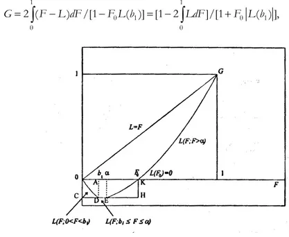
1 1 1 0 0 0 0 2 ( ) 1 2 1 2 2 ( ) 2 [ ( ) ( )] ( ) E K V G F L dF LdF FdL E K F k L k f k dk & ! " " ! " ! " ! + " " !
/
/
/
/
(11)Replacing in the fourth term of (11) the Lorenz curve derived in (10) for the Pareto law, we have the Gini ratio
1/(2 1), 1, [0,1]
G" ! # G0 (12)
2.2. Pareto Type II Model
Pareto (1896, 1897) specified also the Type II (three-parameter) and the Type III (four-parameter) models to be considered as alternatives to the Type I. The specification of his Type II model is the outcome of a translation of the ordinate. Thus, Pareto added to the Type I model a second scale parameter that, in his own fitting of observed income distributions, showed no statistical significant im-provement over the Type I. This outcome should be expected because Pareto added to his Type I scale parameter k0, another scale parameter a that lacks the power to influence the shape of the distribution which is determined by the ine-quality parameter , while k0 and a determine the origin and the support of the Type II distribution, as can be verified from the mathematical form of the CDF and PDF given below in eqs (13) and (14), respectively.
Stiglitz (1969, p. 396) proposed the Pareto law as the asymptotic distribution arising from a set of rigorous and highly imaginative neoclassical economic as-sumptions. He cogently observed (p. 382, note 2) that the works of Champer-nowne (1953) and Mandelbrot (1961) “suffers from the deficiency that the distri-bution of income is determined by a stochastic process, the character of which seems to have little to do with economic processes themselves”. However, Stiglitz’s neoclassical economic assumptions about savings, reproduction, inheri-tance policies, and labour homogeneity have also little to do with real economic processes.
Atkinson (1975, p.300) sustains that Stiglitz proposed the Pareto Type II, al-though Stiglitz (1969, p.396) derived the asymptotic form of the Pareto Type I model. Adding further restrictive assumptions to those advanced by Stiglitz, At-kinson and Harrison (1978, pp. 212-213) state that, “If the economy has been in permanent steady state growth, with constant r and E, the same for all individu-als”, where r stands for the wealth rate of return and E for earnings, then the dis-tribution of wealth follows the Pareto Type II model.
We now present the Pareto Type II model, with support (k0, ), k0>0. Its CDF is
0 0 0
( ) 1 ( ) ( ) , 0, 0, 1
F k " ! k +a k+a ! k#k # k + #a # (13)
and its corresponding PDF, 1 0 ( ) ( ) ( ) f k " k +a k a+ ! ! (14) being, 0 0 limk k f k( ) /(k a) 0 1
% " + # , and limk%& f k( ) 0" . The first and second order differentials of PDF (14) are
2 0 0 '( ) ( 1)( ) ( ) 0, , f k " ! + k +a k+a ! ! , *k#k (15) 3 0 0 ''( ) ( 1)( 2)( ) ( ) 0, . f k " + + k +a k+a ! ! # *k#k (16)
As for the Pareto law, it follows from (14)-(16) that the Pareto Type II PDF is a monotonically decreasing and convex function of k. It decreases from /(k0+a) when k" k0$, to zero when k !. Hence, as the Type I, the Type II model is zeromodal.
The moment of order r about the origin, for r < , is
0 1 0 ( r) ( ) r( ) , r k E K k a k k a dk . & ! ! " " +
/
+ (17)and making the substitution x = k+a, we obtain,
0 0 0 ( )r r ( 1)i i( ) /(i ), . r i r k a a k a r i r i . ! " 2 3 " + ! 4 5 + ! + , 6 7
8
(18)It can be proved that, for any negative integer -r, 0 0 1 ( ) r i i/( ) r i r i k a a r i i .! & ! ! " + ! 2 3 " 4 5 + + + 6 7
8
where ( 1)i r r i 1 i i ! + ! 2 3 2 3 ! 4 5 4" 56 7 6 7, i.e., the negative binomial coefficient is expressed in terms of an ordinary binomial coefficient.
For r = 1 and 2, we deduce from (18),
1 E K( ) (a k0)/( 1), 1, . " " + ! # and (19) 2 2 2 0 0 2 2 0 ( ) ( ) [1/( 2) 2 ( )/( 1) ( ) / ], 2. E K k a a k a a k a . " " + ! ! + ! + + + # (20)
As the Pareto law, it follows from (18) that the Pareto Type II has finite mo-ments of order r only for r< , hence, it is also a heavy tail distribution.
Replacing in (9) the mean wealth from (19) and from (13) the solution of k as a function of F, we derive the Lorenz curve of the Pareto Type II model,
( 1)/
0 0
( ) ( 1)/( ){ ( )[1 (1 ) ]/( 1)}.
L F " ! a+ k !aF+ k +a ! !F ! ! (21)
Replacing L(F) derived in (21) into the fourth term of (11), we obtain the Pareto Type II Gini ratio
1 0 0 0 0 1 2 1 ( 1)/( ) 2 ( 1)( )/(2 1)( ) G" !
/
LdF" +a ! a+ k ! ! k +a ! a+ k (22) Making a = 0 in eqs. (13) to (16) and (18) to (22) we obtain the Pareto Type I results derived in eqs. (2) to (8), (10) and (12), respectively.Although the Pareto Type III was not so far proposed as a wealth distribution model we present it here for its historical interest. Its CDF is
0 ( ) 0 0 ( ) 1 ( ) ( ) , 0, 0, 0, 1. k k F k k a k a e k k k a 9 9 ! ! ! " ! + + # # + # # # (23)
It can be proved that the PDF of the Pareto Type III model is also zeromodal. Moreover, the four-parameter Type III model (23) has only one shape parameter and three scale parameters (a, k0, %). The latter do not contribute to change the shape of the distribution which is determined only by . In effects the scale pa-rameters k0 determines the origin of the support (k0, ) of the distribution, a de-termines the translation of the ordinate, and % the speed of convergence of F(k) to one. For this reason, Pareto (1896) was unable to obtain statistically significant improvement of the fitting of his Types II and III with respect to his Type I model.
2.3. The Lognormal Distribution
McAlister (1879) is considered to be the first scholar that specified the log-normal distribution. His contribution was an outgrowth of Galton’s suggestion. Afterward, Gibrat (1931) specified and applied the lognormal as a two-parameter income distribution model (Dagum 1980, 2001). For the wealth variable K, the lognormal PDF f(k; µ, &2) is obtained from the normal distribution N(x; µ,&2) as a probability generating function and the monotone transformation x = logk. Therefore, 2 2 2 2 1 1 1 exp (log ) , 0; ( ; , ) 2 2 0, 0. k k f k k k . . : : ; : ' <! ! = # > ? @ "( A B > $ ) (24)
Hence, the support of this distribution is (0, ) and its CDF is
2 2 0 ( ; , ) ( ; , ) [(log )/ ;0,1], k F k . : "
/
f z . : dz"N k!. : (25) with parameters(log ) log ,
E K Mg
." " and 2 var(log )
K
: " (26)
where Mgis the geometric mean of K.
It can be proved (Dagum 1980, 2001) that the moment of order r about the origin is equal to the moment generating function of the normal distribution N(k; µ, &2). In effect, 2 2 1 ( ) ( ) exp , 2 r rK r E K E e r r . " " " 24 .+ : 35 6 7 (27) hence, 2 1 1 ( ) exp , 2 E K . " " 24.+ : 35 6 7 (28) 2 2 2 E K( ) exp 2( ), . " " . :+ and (29) 2 2 2 2 1
var( )K ". !. "(exp: !1)exp(2. :+ ). (30)
It follows from (9), (24) and (28) that the lognormal Lorenz curve is
2 2 2 0 2 2 2 1 ( ( )) (1/ )exp[ (log ) / ]/( 2 ) 2 ( ; , ) [(log )/ ;0,1]. k L F k z z dz F k N k . : : : . : : . : : ; " ! ! ! " " + " ! !
/
(31)Therefore, the lognormal Lorenz curve (31) is equal to the lognormal CDF with parameters µ+&2 and &2.
From the first and last members of (25) and (31) we deduce
1( ) (log )/ ,
N! F " k!. :
1( ) (log 2)/ ,
N! L " k! !. : :
hence, the cartesian representation of the Lorenz curve is
1( ) 1( ) .
N! L "N! F !: (32)
It follows from (11), (25) and (31) that the Gini ratio is 1 2 2 2 0 0 1 2 1 2 ( ; , ) ( ; , ), G LdF F k . : : dF k . : & " !
/
" !/
+ (33)where the last integral in (33) is the convolution of the random variable u/v ! 1, where u and v are lognormally distributed with log-medians µ + &2 and µ,
respec-tively, and common variance of logk equal to &2. Hence, it is also a lognormal dis-tribution with log-median &2 and variance of the logarithms equal to 2&2, there-fore,
2 2
1 2 (1; , 2 ) 2 ( / 2;0,1) 1.
G" ! F : : " N : ! (34)
Since Gibrat (1931) brought to the fore the lognormal as an income distribu-tion model and until the earlier 1970s, it attracted the interest of a wide group of applied economists, statisticians and econometricians. Sargan (1959) proposed the lognormal as a model of wealth distribution. Based on rigorous and very unrealis-tic assumptions and after performing a large truncation on the left of the British wealth distribution presented in Langley (1950), he concluded (p. 568) that “the distribution of wealth tends to be approximately lognormal”.
In economic history, the lognormal model was and continues to be a poor rep-resentation of observed income distributions. A fortiori, it is a completely inap-propriate model of observed wealth distributions. It is a very rigid model to be able to accurately represent income and wealth distributions. Moreover, wealth distributions, besides being heavy tail, are dominantly zeromodal, while the log-normal is: (i) a unimodal distribution, and (ii) its log-transformation gives the normal distributions, which is a unimodal and symmetric distribution. Further-more, (27) tells us that the lognormal distribution has finite moments of all orders while income, and a fortiori, wealth distributions are heavy tail distributions. Hence, the specification of income and wealth distribution models must have a finite number of finite moments of positive orders.
2.4. The Loglogistic Distribution
Champernowne (1952) and Fisk (1961) proposed a two-parameter loglogistic distribution as a model of income distribution. Dagum (1975) specified a three-parameter loglogistic; the third three-parameter accounts for the frequency of economic units with income in the neighborhood of zero. Atkinson (1975) considered as models of wealth distribution, the two-parameter loglogistic and the lognormal. He made a graphical fit to the 1968 British net wealth over £ 1000, which repre-sented only a 30.2% of the adult population (18 years old and over). The British net wealth distribution was estimated applying the census multiplier to the estate duty returns. Hence, 69.8% of the adult population was left out, including a 56.1% that were not covered by the estate duty returns. Among the 69.8% adult population there is a high frequency of units presenting negative and null net wealth.
The two-parameter loglogistic CDF and PDF take the forms, 1 ( ; , ) (1 ) , 0, 0, 1; F k C " +Ck! ! k# C# # (35) 1 2 ( ; , ) (1 ) . f k C "C k! ! +Ck! ! (36)
Unlike the Pareto Types I, II and III that are zeromodals, the lognormal and loglogistic, as models of income and wealth distribution, are unimodal. In effect, the modal value M0 of the loglogistic PDF (36) is
1/ 1/
0 [( 1)/( 1)] , 1
M "C ! + # (37)
Although, as a PDF, the loglogistic is defined for all >0, hence it becomes ze-romodal for all belonging to (0,1], as an income and wealth distribution model it has to be >1 for the expected mean value to exist, therefore, for the existence of the Lorenz curve and the Gini ratio, which are validated by factual evidences. Then, as an income and wealth distribution model it is always unimodal. In syn-thesis (Dagum, 1977), the loglogistic is a very rigid model because of its unimo-dality, and because its implies that the income and wealth elasticities with respect to the CDFs F(y) and F(k), respectively, is a linear decreasing function of F.
The moment of order r about the origin (Dagum, 1975) is /
( r) r (1 / ,1 / ), .
r E K B r r r
. " "C + ! ,
It can be proved (Dagum 1975, p. 198) that
/ (1 / ,1 / ) / /sin( / ), ,
r r
r B r r r r
. "C + ! ";C ; , (38)
and its mathematical expectation is 1/
1 E K( ) /sin( / ), 1.
. " ";C ; # (39)
The inverse function of the CDF, i.e., the F quantile, is
1/ 1 1/
( ) ( 1) .
k F "C F! ! ! (40)
It follows from (9), (35), (39) and (40) that the loglogistic Lorenz curve is
( ( ; , )) ( ;1 1/ ,1 1/ )/ (1 1/ ,1 1/ ),
L F k C "B F + ! B + ! (41)
where the complete beta function in (41) is obtained from (38) and (39), i.e., B(1+1/,1-1/ )='/sin('/ ).
It follows from (11) and (41) that the Gini ratio of the loglogistic model is 1
0
1 2 1 2 (2 1/ ,1 1/ )/ (1 1/ ,1 1/ ) 1/ , 1.
G" ! +
/
FdL" ! + B + ! B + ! " #(42) Hence, G=G( ) "1 when "1#, and G( )"0, when " , being a shape pa-rameter and ( a scale papa-rameter.
2.5. Pearson Type V Distribution
Vinci (1921) proposed the Pearson Type V as a model of income distribution. Vaughan, in his University of Cambridge Ph.D. dissertation (Atkinson and Harri-son, 1978 p. 222) specified the Pearson Type V as a model of wealth distribution. In the Pearson system, the Type V PDF takes the form
/
( ; , ) k, 0, 1, 0,
f k C "Ak e! !C k# # C# where A satisfies the area condition, therefore,
/ 1 1 0 1 k ( 1), / ( 1), A k e C dk AC A C & ! ! ! +D ! D "
/
" ! " ! hence 1 / ( ; , ) k/ ( 1) f k C "C !k e! !C D ! (43) and its CDF is 1 / 0 ( ; , ) [ / ( 1)] 1 ( / ; 1)/ ( 1), k z F k C " C ! D !/
z e! !C dz" !D C k ! D ! (44)where is a shape parameter and ( a scale parameter.
It follows from the first and second order differentials of (43) that the Pearson Type V is a unimodal distribution. Its modal value M0 is
0 /
M "C (45)
It can be verified that the Pearson Type V moment of order r is
/[( 2)( 3)...( 1)], 1,
r
r r r
. "C ! ! ! ! , ! (46)
i.e., the Pearson Type V model has finite moments for all r < -1, hence, it is a heavy tail distribution. Its mean and variance are,
1 /( 2), 2,
. "C ! # (47)
2 2
vark"C /[( !2) ( !3)], # 3. (48)
It follows from (9), (43) and (47) that the Pearson Type V Lorenz curve is
2 1 / 0 ( ( ; , ) [ / ( 2)] 1 ( / ; 2)/ ( 2), 2. k x L F k x e dx k C C C C ! D ! + ! D D " ! " " ! ! ! #
/
(49)Being the Lorenz curve a CDF, the PDF of (49) is,
2 1 /
/ [ / ( 2)] k ( ; , 1).
dL dk" C ! D ! k! + !e C " f kC ! (50)
Hence, the Lorenz curve (49) and its PDF (50) are the CDF and PDF of the Pearson Type V with parameter ( and -1 which are deduced from the Pearson Type V PDF (43) with parameters ( and .
The corresponding Gini ratio is 1
0
1 2 ( ( ; , 1) ( ; , ) 1 2 ( ),
G" !
/
L F kC ! dF k C " ! P x$ y (51)hence, it follows from (49) and (44) that
( ( ; , 1)) 1 ( / ; 2)/ ( 2), d x L F k" C ! " !D C k ! D ! (52) ( ; , ) 1 ( / ; 1)/ ( 1), d y F k" C " !DC k ! D ! (53)
where the symbol " stands for equal in distribution. Moreover, G is equal to one d minus twice the convolution of the Pearson Type V Lorenz curve and CDF with shape parameter -1 and , respectively, and common scale parameter (. There-fore, the Gini ratio (51) becomes,
0 1 2 ( / ; 2) ( / ; 1)/[ ( 1) ( 2)] G C k d C k & D D D D " ! +
/
! ! ! ! (54)where the integral is the convolution of two (one- parameter) gamma PDFs with parameters -2 and -1, respectively.
2.6. Dagum Model of Income and Wealth Distribution
Dagum (1977) specified a three-parameter (Type I) and a four-parameter (Type II, when 0, , , and Type III when E 1 E, ) model of income distribution. Da-0 gum (1978b) applied his Type II model to analyze the wealth distribution in Can-ada, Great Britain and the U.S.A. showing an exceptional goodness of fit. Dagum (1990, 1994) made further development of his model to analyze the household and personal distributions of income, net wealth, total wealth, human capital, and total debt. Dagum (1999, 2004) made a comprehensive presentation of his gen-eral model of income and wealth distribution, where the support of net wealth distribution is the set R " !& &( , )of real numbers, thus allowing the fitting of the subset of economic units with null and negative wealth.
The general model and its particular cases (Types I, II and III) are supported by economic and stochastic foundations. Its economic foundation arises (Dagum
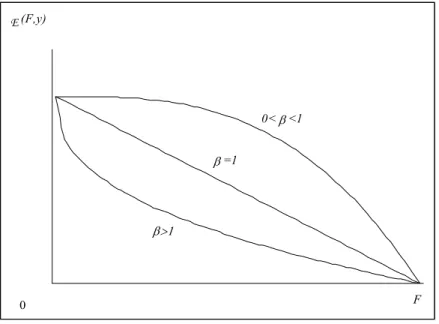
1977) from the observed stable regularity of income, net wealth and total wealth elasticities ( , )F F x of the CDF ( )F G with respect to the corresponding variable X. This factual evidence is also showed for the distribution of human capital and total debt. For the non-negative values of these variables their elasticities were nonlinear and decreasing functions of F, starting from a positive and finite value
1 0
9 # for the lower bound of the positive domain of X, and tending to zero when x % & , henceF %1. Fig. 1 shows the typical shapes of ( , )F F x with re-spect to F.
Taking into account the empirical and stable regularity of ( , )F F x and the ob-served vectors of income and wealth distribution, Dagum (1977) specified the following differential equations.
(a) Type I model
2
1 1 2
( , ) ( / )(F x x F dF dx/ ) (1 F9 ),x 0,( , ) 0.
F " "9 ! # 9 9 # (55)
The solution of (55) gives the Type I CDF
2 1 2
( ) (1 ) , 0, 1/ , 1, 0;
F x " +Cx! !9 x # 9 " 9 "9 9 # C# (56)
being A
e
C" , where A is a constant of integration, hence, C# . 0 (b) Types II and III model
2 1 0 1 2 ( , ) [ /( ( ) )] ( )/ {1 [ ( ) ]/(1 )} , 0, 1,( , ) 0. F x x F x dF x dx F x x x 9 F E E 9 E E E 9 9 ! " ! " ! ! ! # - , # (57)
The solution of the differential equation (57) is
2 1 2
( ) (1 )(1 ) , 1, 1/ , 1.
F x " + !E E +Cx! !9 E , 9 " 9 "9 9 # (58)
For E " , hence 0 x "0 0, we obtain from (57) the differential equation (55), and from (58) the three-parameter Type I model (56). Furthermore:
(b.1) for 0, , , (58) gives the four-parameter Type II model E 1
( ) (1 )(1 ) , 0,0 (0) 1,( , ) 0, 1.
F x " + !E E +Cx! !9 x- , "E F , 9 C # # (59)
(b.2) for E , , we have the four-parameter Type III model with support 0
0 0 (x , ),& x # 0, 0 0 ( ) (1 )(1 ) , 0, 0,( , ) 0, 1, ( ) 0. F x " + !E E +Cx! !9 x-x # E, 9 C # # F x " (60) The greatest lower bound of the support (x &0, ) of the Type III model is the value x0 such that F x( 0) 0," i.e.,
1/ 1/ 1/
0 [(1 1/ ) 1]
x "C ! E 9 ! ! (61)
Translating the ordinate ( )F x to the new origin x "x0, the Type III model (60) admits the following representation
0 0
( ) (1 ( ) ) , 0.
F x " +C x!x ! !9 x #x # (62)
The economic foundation of Dagum model led to the specification of the dif-ferential equation (57). When E " , we obtain the differential equation (55) 0 whose solution is the Type I model (56). These differential equations interpret the contemporary labour market theory characterized by a vertical structural theory of social classes and social mobility. This economic rationale incorporated in (55) and (57) provide the bases for the stochastic foundation of Dagum model. It is the outcome of a set of assumptions specified with respect to the infinitesimal mean and variance of a continuous stochastic process in time and states given by the Kolmogorov forward equations
2 2 ( , ) 1 [ ( , ) ( , )] [ ( , ) ( , )] 2 f z t a z t f z t b z t f z t t z z H H H H " H !H (63)
where ( , )f z t is the PDF of z"logx at time t, x is the economic variable (in-come, wealth or human capital) considered in (57), and ( , )b z t and ( , )a z t stand for the instantaneous mean and variance at time t (Dagum and Lemmi 1989, Da-gum 2004).
The CDF of Dagum Types I, II and III model has a closed mathematical form. Moreover, the inverse function xp, for ( )F x " , is by definition the p-th per-p centile of this model, and has also a closed mathematical form. In effect,
(i) for the Type I CDF (56)
1/ ( 1/ 1) 1/ , 0;
p
x "C p! 9 ! ! p# (64)
(ii) for the Type II CDF (59)
1/ {[(1 )/( )] 1/ 1}1/ 0 1, 0 , hence, 0. p p p x p x 9 E E E E E C ! ! ' ! ! ! , , $ > " ( $ " >) (65.a)
Making p "1/ 2 in (64) we have the median of the Type II CDF (59)
1/ 1/ 1/2 {[(1 )/(1/ 2 )] 1} 0 1/ 2, 0 1/ 2. x 9 C E E E E ! ' ! ! ! , , > " ( ->) (65.b)
given by (65.a), but now we have 0, $ and p 1, F x( 0) 0" , where x0 is given by (61).
The Types I, II and III PDFs present also closed mathematical forms. They are, Type I: 1 1 ( ) (1 ) f x "9C x! ! +Cx! ! !9 (66.a) Type II: 1 1 (1 ) (1 ) , 0 ( ) , 0; and 0, x<0. x x x f x x 9 E E 9C C E ! ! ! ! ! ' + ! + # > "( " > ) (66.b) Type III: 1 1 0 0 0 (1 ) (1 ) , 0; ( ) 0, , where is given by (61). x x x x f x x x x 9 E E 9C ! ! C ! ! ! ' + ! + # # > " ( $ >) (66.c)
Dagum model, in its three Types, has the flexibility to fit zeromodal and uni-modal distributions. It can be showed that the solution of the first order deriva-tives of the PDFs (66) equalized to zero, if they exist, give the modal value,
1/ [( 1)/( 1)] ,1/ 1,
M
x "C 9 ! + 9 # (67)
hence, for 9 # , the Types I, II and III PDFs are unimodal, while for 1 0,9 $ , they are zeromodals. 1
The mathematical expectation, the r-th order moment about the origin ( r , ), the Lorenz curve and the Gini ratio corresponding to Dagum Types I, II and III are derived in Dagum (1980). For the Type II ( 0, , ) we have E 1
1/ 1 E X( ) (1 ) B( 1/ ,1 1/ ), 1; . " " !E 9C 9 + ! # (68) / ( r) (1 ) r ( / ,1 / ), ; r E X B r r r . " " !E 9C 9+ ! , (69) 1/ ( ( ;0 1)) {[( )/(1 )] ; 1/ ,1 1/ }/ ( 1/ ,1 1/ ), 1; L F x B F 9 B E E E 9 9 , , " ! ! + ! + ! # (70) (0 1) (2 1) (1 ) ( , )/ ( , 1/ ) ( , , ), 1, G , , "E E! + !E B 9 9 B 9 9+ "GE 9 # (71)
where the Lorenz curve in (70) is a linear transformation of the beta CDF with respect to the variable [( )/(1 )]1/
1 1/! . Making E = 0 in eqs. (68)-(71), we obtain the corresponding equations for the Type I model.
The parameter E is highly relevant to represent the frequency of economic units with net wealth less than or equal to zero and total wealth in the right neighborhood of zero. It is an inequality parameter, as well as 9 and , while C
is a scale parameter. It follows from (71), that the Gini ratio of the four-parameter Type II model can be symbolized G"G( , , )E 9 . It is a monotonic increasing function of E and a monotonic decreasing function of 9 and (Da-gum 1977 and Dancelli 1986), such that,
0 1 lim ( , , )G lim ( , , ) 1,G 9% 1 E 9 " % 1 E 9 " (72.a) lim ( , , ) lim ( , , )G G , 9%& E 9 " %& E 9 "E (72.b) 0 0 lim ( , , ) lim ( , , ) 0.G G 9 E E E 9 E 9 %& %& % % " " (72.c)
Moreover, E, 9 and play specific roles to account for their respective con-tributions to the level of G. As observed above, E accounts for the contribution to the total inequality G of the economic units with negative and null net wealth and total wealth in the right neighborhood of zero. Dancelli (1986) proved that
9 is more sensitive to changes in the distribution of the low and middle wealth and income groups, while is more sensitive to account for changes in the dis-tribution of the upper wealth and income groups. This role of confirms the constraint of .r in (69). In effect, determines the number of finite moments of positive order, hence, the smaller is , the heavier is the right tail of the PDFs (66), and when $ , the variance does not exist. As shown in (72.a), in the 2 limit, when % 1 , 1 G % I1 , and we have the case of perfect inequality. Be-sides, the greater the estimate of , the greater the number of finite moments, and the faster the convergence to zero of the right tail of the PDF, and as shown in (72.c), in the limit, when % & and E%0,G%0, and we have the case of perfect equality.
On the other hand, numerous case studies of income distribution showed that, for developing countries, 9 tends to be greater than one, hence, the elasticity (Fig. 1) is a decreasing and convex function of F, while for highly industrialized countries 9 tends to be less than one, hence, the elasticity (Fig. 1) is a decreasing and concave function of F. Moreover, for highly industrialized countries, the wealth distribution estimates of 9 tend to be less than the estimates of their cor-responding income distributions. The reverse relationship between developed and highly industrialized counties is observed for ; in effect, for highly industri-alized countries, the estimates of are systematically larger than those of the de-veloping countries. Hence, among dede-veloping countries, the low and middle
in-come groups present less inequality, and the high inin-come groups more inequality than the highly industrialized countries. These empirical facts reveal that the de-veloping countries present a larger polarization of income, therefore, less equity, than the highly industrialized countries. The dearth of wealth distribution data among developing countries does not allow a similar analysis about the relative levels of 9 and . However, the poor and inefficient functioning of their institu-tions, in particular, the Judicial power, allows to infer that most developing coun-tries present a higher concentration of wealth, i.e., a smaller , than the highly industrialized countries. 0 9=1 9#J 0<9<1 F E (F,y)
Figure 1 – Income elasticity $(F,y) of the CDF F(y).
The relative values of 9 and between developing and highly industrialized countries can be inferred from the income elasticity of the CDF in Fig. 1. In ef-fect, its convexity for developing countries shows a fast initial decrease of the elasticity followed by a slow decrease for the high income groups. Instead, the concavity shape of the elasticity for highly industrialized countries shows a slow initial decrease followed by a fast decrease.
As far as I know, the localized, hence, the differentiated roles played by the inequality parameters E, 9 and is a unique feature of Dagum model among the specified income and wealth distributions. Moreover, being G"G( , )9 for the Type I, and G"G( , , )E 9 for the Type II and III model, the presence of at least two inequality parameters allows the detection of intersecting Lorenz curves. This is possible because of the specialized roles of E, 9 and .
and Kleiber and Kotz 2003). Kleiber’s Theorem 2 states that, given two Dagum random variables X1 and X2 such that
( , , ), 1, 1, 2, d i i i i X "D 9 C # i" then 1 2 1 2 1 1 2 2 (X -L X )K( $ and 9 $9 ) (73)
where X1-L X2 stands for “Lorenz curve of X1 nowhere above that of X2”. Kleiber’s Theorem 2 enriches the interpretation of the inequality parameters and
9 given above. This type of analysis cannot be done when working with two-parameter income and wealth distributions where one is a scale and the other a shape (inequality) parameter such as the lognormal, loglogistic and gamma models. In these cases, the Gini ratio is a monotonic increasing function of the inequality parameter of lognormal and gamma models and a monotonic decreas-ing function of the loglogistic. Hence, increasdecreas-ing values of the inequality parame-ter imply a displacement to the right in the Lorenz curve for the first two distri-butions, and to the left for the latter.
Given Kleiber’s Theorem 2 and taking into account the specific roles played by the inequality parameters and 9 , we can state that, if
1 2, 1 2, and 1 1 2 2
9 $9 # 9 #9
then the Lorenz curve L2 intersects from above the Lorenz curve L1. Moreover, the economic units in the neighborhood of the intersection point contribute to increase the income or wealth shares of the economic units to the left and the right of that neighborhood.
2.7. Dagum General Model of Net Wealth Distribution
Dagum (1990, 1993, 1999, 2004) generalized his income and wealth distribu-tion model specifying a model of net wealth distribudistribu-tion with support (!& & to , ) account also for the high observed frequencies of negative and null net wealth. Furthermore, it contains as particular cases Dagum Type I, eq. (56), and Type II, eq. (59).
Unlike the right tails of income and (net and total) wealth distributions which present heavy tails, the left tail of net wealth distributions, i.e., when the net wealth tends to minus infinity, present a fast convergence to zero because of in-stitutional and biological bounds to an unlimited increase of the economic agents’ liability.
The stylized facts outlined above determine the specification of a net wealth distribution model as a mixture of an atomic and two continuous distributions. The atomic distribution, F x2( ), concentrates its unit mass of economic agents at
0
x " . It accounts for the economic units with null income, net wealth and total wealth. The continuous distribution F x1( ) accounts for the negative net wealth observations. It has a fast left tail convergence to zero, hence, it has finite mo-ments of all orders. The other continuous distribution,F x x #3( ), 0 accounts for the positive values of income, net wealth and total wealth and presents a heavy right tail, therefore, it has a small number of finite moments of order r #0. Sometimes, for net and total wealth, the variance might become infinite. F x3( ) is specified as the Dagum Type I model.
The symbolic notation of the net wealth distribution model as a mixture of an atomic and two continuous distributions takes the form
1 1 2 2 3 3 1 3 2 1 2 3 ( ) ( ) ( ) ( ), ,( , ) 0, 0, 1 F x b F x b F x b F x x b b b b b b " + + !& , , & # - + + " (74)
and its mathematical specification is,
1 2 3 3 1 2 ( ) exp( ) max{0, / } (1 ) , , min{ , 0}, max{ ,0},( , , , ) 0, 1, 1 , , s F x b c x b x x b x x x x x x c s b b b 9 9 E E C C ! ! ! + ! + " ! + + + !& , , & " " # # " ! + " (75) where, 1
1( ) exp( ), ( )1 exp( )( 1)min{ / , 0};
s s s F x " !c x! f x "cs x! ! !c x! ! x x (76.a) 2( ) max{0, / }, (0) 1 and ( ) 0,2 2 0; F x " x x! f " f x " *x L (76.b) 1 1 3( ) (1 ) , ( )3 (1 ) . F x " +Cx+! !9 f x "9C x+! ! +Cx+! ! !9 (76.c) Furthermore, and c C are scale parameters and all the others, i.e. b1, b2, b3, s, 9 and are inequality parameters. b b1, and 2 s account for the contribution to the Gini ratio of the negative and null net wealth observations, while b3, and 9 ac-count for the contribution to the Gini ratio of the positive net wealth observations. In general, all observed net wealth distributions present positive frequencies of negative, null and positive net wealth, i.e., ( , , ) 0b b b1 2 3 # , where bi is the weight of ( ),F x i "i 1, 2, 3, in (74) and (75) such that,
1 ( 0), 2 ( 0), 3 1 ( 0).
b "P x, b "P x" b " ! "E P x#
Therefore, at x"0, ( )F x present a point of discontinuity with a finite jump equal to b2 (Fig. 2). Should we get an estimate b "2 0 (Fig. 3), then F(x) is a con-tinuous function for all x 0 !& & , presents a kinked point at x=0, and is dif-( , ) ferentiable everywhere but at x=0.
0 b1=F1(w ) E+(1-E)F3(w ) b1 E=b1+b2 w F(w )
Figure 2 – Cumulative distribution function of a net wealth distribution, 0<b2<1.
Figure 3 – Cumulative distribution function of a net wealth distribution, b2=0.
Given the mathematical structure of the specified net wealth distribution model (75) and (76), it can be proved (Dagum 1990, 1999, 2004) that
1 1/ 1/ 1 ( ) (1 1/ ) (1 ) ( 1/ ,1 1/ ), 1 s E X b c s B . E 9C 9 ! D " " ! + + ! + ! # (77) / / 1 ( r) ( 1)r r s (1 / ) (1 ) r ( / ,1 / ), . r E X b c r s B r r r . " " ! ! D + + !E 9C 9+ ! , (78) For the Lorenz curve we have,
1/
1 1 1 1 1 1
( ;0 ) ( ) s[ (1 1/ ) (log( / );1 1/ )]/ ;
L F , ,F b "b L F " !b c! D + s !D b F + s .
(79) (ii) for F "b1, hence, x% I 0 :
1/
1 1 1
( ) s (1 1/ )/ ;
L b " !b c! D + s . (80)
(iii) for b1,F $E, hence, x=0: 1/
1 1 1 1
( ; ) ( ) s (1 1/ )/ ;
L F b , $F E "L b " !b c! D + s . (81)
(iv) for F #E, hence, x>0:
1/ 1/ 1/ 1 1 ( ; ) [(1 ) [(( )/(1 )) ; 1/ ,1 1/ ] s (1 1/ )]/ . L F F B F 9 b c s E E 9C E E 9 ! D . # " ! ! ! + ! ! + (82) It follows from (82) that for F "1, (1) 1L " . Fig. 4 illustrates the shape of the net wealth Lorenz curve.
Taking into account the presence of negative values of the Lorenz curve in the interval (0,F0), where F0 is the point of intersection of L(F) with the abscissa F, i.e., is the solution of the equation L F F( ;0 0 #E) 0" in (82), we define the Gini ratio as follows: 1 1 0 1 0 1 0 0 2 ( ) /[1 ( )] [1 2 ]/[1 ( ) ], G"
/
F!L dF !F L b " !/
LdF +F L b (83)i.e., twice the integral between the equidistribution function L=F and the Lorenz curve divided by one plus the area of the rectangle OCHK in Fig. 4.
It can be verified that, (i) when b1"0, then b2" and we have the Dagum E Type II model; and (ii) when b1" b2"0, hence E "0 and b3" ! " we 1 E 1, have the Dagum Type I. The Type II is a general model of total wealth distribu-tion. It is also relevant when fitting net wealth distribution data in the closed-open interval [0, )& , where E" +b1 b2 "P x( $0). Dagum three-parameter Type I model can present an excellent goodness of fit of both net and total wealth data in the interval [0, )& when these distributions are zeromodal, i.e., 0,9 $ , and 1 the frequency E" + is high, in general over 20% of the population, being b1 b2
1 0
b # for net wealth and b "1 0 for total wealth. In (75), if we specify b "1 0 and allow b2" to be less than zero, i.e.,E b2 " , , we obtain the Dagum Type III E 0 model with support ( , ),x0 & x0 #0, such that (F x0) 0" . It is highly relevant to fit the human capital distribution and, for some socioeconomic attributes, for stance, the occupied member of the labour force, it is also relevant to fit the in-come distribution. Therefore, depending on the attribute considered, which has to do only with the lowest income group, one of the three types of Dagum model is the most relevant to fit observed income distributions.
3. ESSENTIAL PROPERTIES OF INCOME AND WEALTH DISTRIBUTIONS
Dagum (1977) introduced and analyzed 14 properties to guide the choice of an income distribution model. Those properties are highly relevant to support the choice of net wealth, total wealth, human capital and total debt distribution mod-els. We introduce here the following eight essential properties:
P.1. Model foundation;
P.2. Convergence to the Pareto law;
P.3. Existence of only a small number of finite moments; P.4. Economic significance of the parameters;
P.5. Model flexibility to fit both unimodal and zeromodal distributions;
P.6. Model flexibility to fit distributions with support
0 0
(0, ),[0, ),( , ),& & x & x #0, and (- , );& &
P.7. The parametric Lorenz curve and Gini ratio derived from an estimated model should be able to account for intersecting Lorenz curves; and
P.8. Parsimony.
These properties are now considered to assess the relative validity of the wealth distribution models discussed in Section 2.
P.1. Model foundation. The specification of any model purporting to describe and explain basic features of an aspect of reality has to be supported by a theoretic-empirical foundation, i.e., by a set of realistic and elementary assumptions ac-counting for the empirical regularity and stability of the phenomena object of
cognition. Moreover, given the stochastic nature of wealth distribution processes, the specified models should have also a meaningful (not a purely random) sto-chastic foundation.
P.2. Convergence to the Pareto law. Theoretic-empirical research (Macaulay 1922, Davis 1941, Mandelbrot 1960, and Ord 1975) support the specification of the Pareto law as the model of high income groups, and a fortiori, we retain it as the model of high net and total wealth groups, for instance, the last quantile.
A net or total wealth distribution model weakly converges to the Pareto law if it tends to the Pareto Type I model for high wealth groups. In symbols,
0 0
[1!F x( )]/( /x x )! %1 when x% & ,,0 x ,x, # 1, (84) hence, for high wealth values of x0,1!F x( ) tends to( /x x0) ,! x #x0. P.3. Existence of only a small number of finite moments. Although P.2. and P.3. over-lap, since both properties imply that the specified model belongs to the class of heavy tail distributions, I keep them separated to distinguish between the prop-erty of convergence to the Pareto law and the existence of a small number of fi-nite moments with or without infifi-nite variance. Manderbrot (1960) argued that distributions of monetary variables, such as income and wealth, have infinite vari-ance, hence, they belong to the Lévy stable law. However, overwhelming empiri-cal evidences show that, since 1950, income distributions tend to have finite vari-ance, and very often finite moment of order three, and sometimes of order four, while wealth distribution models tend to be zeromodals, and sometimes the vari-ance is infinite.
P.4. Economic significance of the parameters. The parameters of wealth distribution models should have a clear and unambiguous economic interpretation of both scale and shape (inequality) parameters. The former change with changes of the variable unit of measurement and the latter are dimensionless parameters.
P.5. Model flexibility to fit both unimodal and zeromodal distributions. Since the industrial and French revolutions of the XVIII Century, it started a sustained process of technological and institutional development that induced a process of structural changes in the mode and social relations of production, generating a slow decreas-ing trend in income and wealth inequalities. It lasted until the 1970s when a trend reversal started. Furthermore, in the XX Century, the shape of the income distribu-tions of many countries passed from zeromodal to unimodal and from infinite to finite variance. Instead, net and total wealth distributions continue to be dominantly zeromodal and several of them still have infinite variance. For these reasons, be-sides P.2 and P.3, income and wealth distribution models have to have the flexibil-ity to fit zeromodal as well as unimodal distributions.
P.6. Model flexibility to fit distributions with support (0, ),[0, ),(& & !& &, ) and
0 0
(x ,&), x #0. The support (0, )& is the general case of models dealing with observed income distributions. However, there are many instances where the support should be [0, ) or ( , ),& x0 & x0#0, depending on the economic con-juncture (stage of the business cycle) and the socioeconomic attribute under
in-quiry (households, adult individuals, members of the labour force, households head by gender, etc.). Besides, the support (x0, ),& x0# seems to be the gen-0, eral case of human capital distributions (Dagum 1994, Dagum and Slottje 2000, Dagum et al. 2003). Instead, the support [0, )& is the general case of total wealth distribution, where (0)F "E,0, , because of the high frequency of eco-E 1, nomic units with total wealth in the right neighborhood of zero. When the esti-mate of E is high and the wealth distribution is zeromodal,
Dagum Type I model with support (0, )& can be fitted to the data. The sup-port [0, )& is also relevant to fit net wealth distribution data, where
( 0)
P X
E " $ estimates the total frequency of economic units with null and negative net wealth. When we have the sample surveys data of the economic units with negative, null and positive net wealth, then the general model (75)-(76) with support (- , )& & is retained.
P.7. The parametric Lorenz curve and Gini ratio derived from an estimated model should be able to account for intersecting Lorenz curves. This property requires that the income and wealth distribution models present at least two inequality parameters. This property is enhanced when, as in Dagum Types I, II and III model, the inequality parameters have a localized role in the distribution.
Necessary and sufficient conditions for the non-intersection of Lorenz curves were studied by Kleiber for the Dagum Type I model, Wilfling and Krämer (1993) for the Sing-Maddala model, and Wilfling (1996), Kleiber (1999) and Sara-bia et al. (2002) for McDonald generalized beta-II distribution.
P.8. Parsimony. This is a general scientific principle. In this study it requires the specification of a model with the smallest possible number of parameters among those that offer an accurate and robust representation of observed income and wealth distributions. Moreover, the specification of three-parameter models should contain one scale and two inequality parameters. Pareto addition to his Type I model of one and two scale parameters to arrive at the specification of his Types II and III model, respectively, does not add a statistically significant im-provement to the model goodness of fit, and furthermore, they cannot detect cases of intersecting Lorenz curves.
Four-parameter models should only be entertained if their parameters have a clear economic interpretation and well determined roles to account for the shape of observed distributions. This is the case of Dagum Types II and III and Dagum general model.
Today advanced state of the information technology allows the mathematical and statistical analysis and fitting of models with five and more parameters. This practice should be abandoned mainly because of the following three compelling reasons: (i) over fitting of the distributions; (ii) do not have a clear and differenti-ated interpretation of the inequality parameters; and (iii) being the income and wealth distribution models univariate functions, they introduce a high and unac-ceptable degree of multicollinearity among the estimated parameters.
4. WEALTH DISTRIBUTIONS MODELS AND THEIR PROPERTIES
We now discuss the fulfilment of the eight properties studied in Section 3 by the wealth distribution models so far specified and analyzed in Section 2.
Table 1 presents the property evaluation of the wealth distribution models dis-cussed in Section 2. This evaluation is also relevant for the assessment of income distributions models.
Pareto Types I and II models, being zeromodals, having the power to fit high in-come and wealth groups only, and having one inequality parameter, do not fulfil P.5, P.6 and P.7. Besides, Pareto Type II does not fulfil P.1 (model foundation).
The lognormal fulfils only P.4 (economic significance of the parameters) and P.8 (parsimony). Gibrat’s model foundation is not acceptable (N.A.) because his law of random proportional effect, criticized by Kalecki (1945) implies, contrary to historical evidences, that income and wealth inequality :2 "var log X follows an increasing trend. In effect, given x0,
2
1 1
logxt "logxt! +Ft! ,Ft"d N(0,: ),cov( ,F Ft t r! ) 0," r L 0, (85) hence,
0 0 1 1
logxt "logx +F +F + +... Ft! , and (86)
2
var(logXt)"tvarFt "t: , (87)
which is an increasing function of t, confirming Kalecki’s critique. Therefore, lognormal income and wealth distribution processes satisfying Gibrat’s assump-tion will never converge to a stable lognormal distribuassump-tion with finite variance. Gibrat’s second assumption states that the standardized normal variate is a linear function of logx, i.e,
1( ( )) (log )/ ,
n
z"N! F x " x!. : (88)
where Fn(x) is the observed CDF obtained from a sample of size n. Empirical evidences show that it is rather a cubic or a polynomial of a higher degree, con-firming Rutherford’s (1955) critique.
The loglogistic model fulfils P.2, P.3, P.4 and P.8. It does not have a model foundation (P.1); as a model of income and wealth distribution we have # , 1 hence it is unimodal (see eq. (37)), and its support is the open interval (0, )& , then it does not fulfil P.5 and P.6. Having one inequality parameter, it does not fulfil P.7.
Pearson Type V model does not fulfil P.1, P.5, P.6 and P.7 because it does not have model foundation, is unimodal, its support is (0, )& , and it has only one inequality parameter. Instead, it fulfils P.2, P.3, P.4 and P.8.
Dagum Type I model (56) fulfils seven out of the eight properties. Because its support is (0, )& , P.6 is partially fulfilled by this model. Should the observed
in-come and wealth distributions require a different support, we can consider, for income distributions, Dagum Type II or Type III; for total wealth distribution, Dagum Type I or Type II; and for net wealth distribution, Dagum Type II model (59) or Dagum general model (75).
Dagum Type II and his general model (75) satisfy the eight essential properties introduced in Section 3.
Finally, it should be stressed that the property of parsimony, i.e. P.8, has to be considered with respect to the specification of each of the CDFs entering in the convex combination (74) and (75).
TABLE 1
Wealth distribution models and their properties
Properties Model
P.1 P.2 P.3 P.4 P.5 P.6 P.7 P.8
Pareto Type I Y YYY Y Y Y NO NO NO Y
Pareto Type II NO Y Y Y NO NO NO Y Lognormal N.A. NO NO Y NO NO NO Y Loglogistic NO Y Y Y NO NO NO Y Pearson Type V NO Y Y Y NO NO NO Y Dagum Type I Y Y Y Y Y NO Y Y Dagum Type II Y Y Y Y Y Y Y Y
Dagum General model Y Y Y Y Y Y Y Y
N.A. stands for “not acceptable”.
TABLE 2
Fitting the Dagum model to the wealth distribution in Ireland, the U.K., Italy and the U.S.A.
1966 Ireland Net Wealth
Distribution in £ 1000 U.K. Net Wealth Distribution 2000 Italy Wealth Distribution in L 106
In £ 1000 In £ 10000 Male Female Total
1954 1970 1990 1992 Net Total
1983 U.S. Net Wealth Distribution in $ 10000
b1 n/a n/a 0 n/a 0.038 0 0.0562
b2 n/a 0.5181 0 0.0335 0.017 0.09 0
!= b1+b2 0 0 0 0 0.5181 0 0.0335 0.055 0.09 0.0562
b3=1-! 1 1 1 1 0.4819 1 0.9665 0.945 0.91 0.9438
C n/a n/a n/a n/a n/a n/a n/a 0.00007 0 3.422
S n/a n/a n/a n/a n/a n/a n/a 1.04 0 0.677
) 0.0553 0.0225 0.0376 0.0321 0.3793 0.2687 0.3897 0.222 0.252 0.207 ( 376.6506 376.5674 376.6345 285.912 24.257 361.10 127.983 87336.8 87341.3 463.85 2.7153 2.8440 2.7145 3.6294 1.8561 2.5672 2.3189 2.835 2.853 2.1823 9 0.1502 0.064 0.1021 0.1165 0.7040 0.6898 0.9037 0.629 0.72 0.4517 x0 0 0 0 0 0 0 0 n/a 0 n/a SSE (PDF) 0.0011 0.0001 0.0003 0.0016 0.0001 0.00067 0.00017 0.00067 0.00187 0.0010 SSE (CDF) 0.0010 0.0003 0.0005 0.0009 0.0001 0.00036 0.00030 0.00413 0.00521 0.0042 K-S 0.0165 0.0064 0.0010 0.0157 0.0012 0.0086 0.006 0.008 0.021 0.023 m 23 23 23 8 29 12 12 31 36 39 Gini ratio 0.8125 0.9057 0.8618 0.8321 0.828 0.5557 0.5532 0.577 0.569 0.681 Observed median 53.20 0.0 0.0 157 0.0 37410 38540 18.0 18.8 33788 Estimated median 87.87 0.156 10.03 12.3 0.0 37427 38901 17.0 18.1 32094
5. APPLICATION
The analysis and property evaluation of the proposed net and total wealth dis-tribution models are illustrated in Table 2 with ten case studies. For seven of them, we work with the published data in the interval [0, ).& They are: 1986 Ire-land net wealth distribution data by gender and total (Lyons, 1974, p. 188) and the 1954, 1970, 1990 and 1992 U.K. net wealth distribution data (U.K. Inland Revenue Statistics, 1994 and former issues). For Ireland, the reported frequencies of null net wealth, which include the economic units with negative net wealth, are: 49.4% for male, 74.5% for female, and 62.0% for the total. Hence, the ob-served female and total median net wealth is equal to zero, while that of male is positive and close to zero.
For the other three case studies, i.e., 2000 Italy net and total wealth distribution (Banca d’Italia, 2002) and 1983 U.S. net wealth distribution (Avery and Ellie-hausen, 1985) we work with the corresponding magnetic tapes which contain the net and total wealth data of each person in the sample surveys. They provide the information of the economic units with negative and null net wealth, hence, the net wealth distribution data of Italy and the U.S.A. belong to the interval
( , )
R " !& & .
Common features of these ten observed wealth distributions are:
i) zeromodals, which continue to be a dominant feature in today national economies, hence, their corresponding PDFs are monotonic decreasing functions;
ii) heavy tail distributions, therefore, they have a finite number of finite mo-ments of order r>0, and sometimes they have infinite variance;
iii) the support of total wealth distribution is the closed-open interval [0, )& ; iv) when we have the data of all the members of a sample survey, the support of net wealth distributions is R " !& &( , ); otherwise, when we have the data by class intervals, the support is [0, )& .
It follows from the analysis and property evaluation of wealth distribution models (Sections 2, 3, 4, and Table 1), and the common features of observed wealth distributions presented above, that:
a) except as a limit case, when fitting the high wealth groups, we have to ex-clude the Pareto Types I and II as a model of wealth distribution because its sup-port is the interval ( , ), where x0 & x0 # , and in general, it is greater than the 0 50th percentile of the distribution, the model is always zeromodal, and it has only one inequality parameter;
b) we have to rule out the lognormal, mainly because of its insufficient model foundation, lacks of convergence to the Pareto law, existence of moments of all orders, hence it presents a fast convergence to zero, and it is a rigid unimodal dis-tribution where the log of wealth is normally distributed;
c) although the loglogistic and Pearson Type V are heavy tail distributions, we have to rule them out because of the lack of economic and stochastic founda-tions, and moreover, because they are unimodal distribufounda-tions, have only one ine-quality parameter and their corresponding support is the interval (0, )& ;