DOTTORATO DI RICERCA IN MATEMATICA XXII CICLO
MAT 07: Fisica Matematica
ENTROPY AND SEMANTICS:
TEXTUAL INFORMATION EXTRACTION
THROUGH STATISTICAL METHODS
Tesi presentata da Chiara Basile
Coordinatore:
Chiar.mo Prof.
ALBERTO PARMEGGIANI
Relatore:
Chiar.mo Prof.
MIRKO DEGLI ESPOSTI
There are more things in heaven and earth, Horatio, than are dreamt of in your philosophy.
W. Shakespeare, Hamlet, act 1, scene 5
L. van Beethoven, Symphony no. 5, Allegro con brio
-GACTGCTTGCATTAAAGGACTTCCTCATC...
Human DNA, chromosome X, gene ODZ1
-When William Shakespeare wrote his masterpieces, he certainly didn’t think that, one day, someone would refer to them as productions; for sure, while typing on his piano keybord, Ludwig van Beethoven didn’t consider himself as an information source; and if we think of the sequence of bases in a gene, our first idea will not be to look for patterns so as to be able to give a shorter description of its structure.
The relationship between information theory and the real world is not immediate, and the risk of confusing the reader is always present. Neverthe-less, a large number of situations in our lives fit into this scheme: someone or something “produces” an output, that can be represented as a sequence of symbols extracted from some finite set; even if we do not know the details of the source, we can reconstruct its properties by looking at the sequence it generated, by extracting as much information as it is possible to deduce
from its content, structure, etc.
Let us go back to Shakespeare’s example: we have few details about his biography, and nevertheless when we read Macbeth or Hamlet we acquire a lot of information about his beliefs, his wit, his idiosyncrasies, his use of words, etc. All of these elements can be included in the single, comprehensive concept of style. And if the normal path for the detection of an author’s style is the study of his bioghaphical and historical background, together with an accurate (human!) reading of his writings, there are a number of properties that can be detected by using automatic or semi-automatic tools. This is exactly the object of research on automatic information extraction from symbolic sequences, a very wide and lively field of information theory, with a quite solid mathematical background and a number of contaminations with other fields of research, as the theory of dynamical systems.
Since most of the information in the world can be represented in terms of symbolic sequences (cf. [13]), the methods and models of information extraction can be applied to a number of cases. Among others, and with no pretension of completeness, we add to the already cited problem of authorship attribution a large variety of text classification tasks (by genre, by topic, ...), the automatic extraction of keywords from long compositions [49, 50] and, stepping away from written texts, the identification of musical pieces from short and noisy excerpts, a number of biological sequence classification problems [8, 20, 52], and the list could be much longer.
Some of the techniques that are used in literature for these and other similar tasks exploit as much as possible the particular structure of the se-quences that are the object of analysis: for example, a written text has an underlying syntactical structure that can be put in evidence by an appro-priate tagging of words or phrases, whereas a piece of music can be studied in terms of its sections, beats, pauses, and so on. The methods that we will apply for information extraction from written texts, instead, will be as much as possible independent from the structure of the texts themselves, and will refer to very general theoretical results in terms of entropy estimation
and statistical properties of the sequence; this is a tendency that is gaining ground in this field, usually through the studies of researchers coming from “pure” sciences like mathematics or physics.
An important remark is that often the study of experimental results leads to interesting considerations about the theoretical framework that underlies the methods, and in our experience the practice of information extraction of-ten requires the use of semi-statistical indicators: asymptotic properties and statistically significant quantities are not often the case in real-world textual corpora, and the study of this “borderline” region may lead to interesting progresses both for theory and for the applications.
Here is the scheme of this thesis.
In chapter 1 we will present the theoretical framework of symbolic se-quence analysis, adopting mainly the language of Information Theory, as founded by C.E. Shannon in [59], but without forgetting the equivalent for-mulation in terms of Dynamical Systems; a very stimulating reading to un-derstand this equivalence is the book by P.C. Shields [60], that was the source of inspiration for a good part of chapter 1. After presenting the definition of information source and discussing the meaning and the central role of prop-erties like stationarity and ergodicity, also for the applications, we will move to data compression and its role in the estimation of the entropy of a source. Data compression is nowadays a very well established field of information theory, thanks to the founding papers published by J. Ziv, A. Lempel and their coworkers in the 1970s (cf., among others, [38, 70, 71] and the review paper [69]), where they proposed a variety of compression algorithms (the family of LZ algorithms), based on the idea of a clever parsing (subdivision) of the symbolic sequence. It was a huge progress in the field, since it was the first example of compressor that doesn’t operate a fixed number of character at a time, but is allowed to vary the length of encoded substrings according to the “size” of the regularities that that specific sequence presents; indeed, such algorithms are still at the base of the most common zipping software that we use everyday on our computers.
In 1993 J. Ziv and N. Merhav [73] proposed a method to estimate the rela-tive entropy (or Kullback-Leibler divergence) between couples of information sources, starting from their realizations: they proved that a modified version of an LZ algorithm, where the regularities for a sequence are searched in another sequence, can be used to approximate the relative entropy between the two sources that generated such sequences. This important result was used in various subsequent studies, among which [8], to deal with problems of text classification and clustering.
Taking advantage of some results on the recurrence of patterns in symbolic strings, that were developed in parallel in the context of dynamical systems (in terms of hitting times for the orbits of dynamical systems, see for example [21]) and with the language of probability and stochastic processes (cf. [33, 34]), we will give a new proof of Ziv-Merhav’s Theorem. Our proof is different from the original one, which is based on heavy probabilistic tools, and also from the one that H. Cai, S.R. Kulkarni and S. Verdú proposed in [11], where they make use of the Burrows-Wheeler transform [10].
With chapter 2 we will move from a purely theoretical setup to the applications to information extraction from written texts. In this chapter we will deal in particular with problems of authorship attribution, using methods that are derived from the results in chapter 1. With this we do not mean that we will directly apply theoretical results of information theory to real-world contexts: as discussed above, indeed, the passage from theory to practice always requires great care and some adaptations to fit the specific problem.
We will describe in this section two experiments with real-world textual corpora. The first is the result of a collaboration between our group, D. Benedetto and E. Caglioti from Rome-La Sapienza, M. Lana from the Uni-versity of Western Piedmont in Vercelli and the Fondazione Istituto Gramsci in Rome. We were asked to give indications about the possibility that a num-ber of short articles, published anonimously on the same newspapers where Antonio Gramsci and his coworkes wrote, are actually pieces of Gramsci’s writing; the Fondazione is passing the results of our study to his team of
expert phylologists, so as to decide whether or not to include those texts in the complete edition of Gramscian works that is in the process towards pub-lication. Apart for the interest of the attribution problem per se, the corpus that was made available to us is a very stimulating one from the point of view of authorship attribution studies, as we will thoroughly discuss in the chapter.
Furthermore, it is interesting to note that our studies, that certainly are out of the mainstream of standard linguistic analysis of texts for authorship attribution purpose, are nonetheless consistent with a tendency that started gaining ground in the last decade or so in this area (cf. [32, 14, 29, 61, 62] and the discussion in [6, in Italian]): the written text, which is the result of a complex combination of semantic, linguistic and historical properties, is deprived of all such structure and considered instead as a mere sequence of symbols from a certain alphabet, on which statistical and semi-statistical methods can be applied to extract stylistic information.
The same tendency has become prominent also in the field of plagia-rism detection, that will be the subject of chapter 3. We move here to a more “technological” application, at the same time very different and sharing similar elements with authorship attribution. Indeed, from a certain point of view the problem of recognizing the authenticity of a written text is certainly a matter of style analysis, and in this it is near to authorship attribution; on the other hand, plagiarism is much more content-related than authorship is (cf. [16]), and also the typical size of a reference corpus for this kind of studies is orders of magnitude larger than a standard real-world authorship attribution data set.
In 2009 the 1st International Competition on Plagiarism Detection [54] was proposed, in order to compare plagiarism recognition methods and tech-nologies on a common ground. We participated in the contest (cf. [4]), and obtained the third position among the ten participating groups: a good re-sult considering that our background on plagiarism detection was practically null. Indeed, we applied there our experience on authorship attribution,
es-pecially for a first selection of the most relevant sources of plagiarism for each suspicious text, which is the first phase of practically any plagiarism de-tection algorithm (cf. [64]). We also developed a couple of interesting ideas to reduce the computational load of the experiments, by using certain lossy codings that allowed for a reduction of the alphabet and, in one case, for a dratic cut of the text length. One of these codings, based on word lengths, is analysed in a certain detail in this chapter, and with greater accuracy in a work with A. Barrón-Cedeño and P. Rosso of the Polytechnic University of Valencia [2]. As we will underline in the conclusions of this chapter, more work needs to be done to reduce the heuristics and to give our methods a better experimental validation in this field.
Most of the numerical experiments for this thesis were performed by using
Introduction i
1 Entropy, relative entropy and pattern matching 1
1.1 Notations and main concepts . . . 1
1.1.1 Basic notations and definitions . . . 1
1.1.2 Entropy and relative entropy . . . 5
1.2 Coding and LZ compression . . . 8
1.2.1 Coding and entropy . . . 8
1.2.2 Universal codes, LZ compressors . . . 10
1.2.3 Ziv-Merhav Theorem for relative entropy . . . 14
1.3 Relative entropy via return times and match lengths . . . 15
1.3.1 Definitions and asymptotical results . . . 15
1.3.2 Relative entropy via return times and match lengths . 18 2 Applications: authorship attribution 21 2.1 Stylometry, from words to n-grams . . . 21
2.2 The Gramsci Project . . . 24
2.2.1 Description of the project and corpora . . . 24
2.2.2 The n-gram distance . . . 26
2.2.3 Entropy and compression: the BCL method . . . 33
2.2.4 The overall procedure and the experiments . . . 37
2.2.5 n-gram statistics . . . 39
2.2.6 Ranking analysis . . . 41
2.2.7 A quick comparison with other methods . . . 46 vii
2.3 Xenophon and Thucydides . . . 49
2.3.1 The problem . . . 49
2.3.2 A first experiment . . . 50
2.3.3 Are simple statistics enough? . . . 52
2.3.4 Extending the corpus . . . 52
2.4 Conclusions and future developments . . . 56
3 Applications: plagiarism 59 3.1 Plagiarism detection . . . 59
3.2 PAN‘09 competition: our method for external plagiarism . . . 62
3.2.1 A general scheme for plagiarism detection . . . 62
3.2.2 The PAN‘09 corpus of external plagiarism . . . 63
3.2.3 A first selection with word length coding . . . 64
3.2.4 Detailed analysis: T9, matches and “squares” . . . 66
3.2.5 Results and comments . . . 71
3.3 Back to the word length coding . . . 72
3.4 Intrinsic plagiarism . . . 75
3.5 Concluding remarks . . . 77
Discussion and perspectives 79
Acknowledgements 81
Entropy, relative entropy and
pattern matching
My greatest concern was what to call it. I thought of calling it ‘information’, but the word was overly used, so I decided to call it ‘uncertainty’. When I discussed it with John von Neumann, he had a better idea. Von Neumann told me, ‘You should call it entropy, for two reasons. In the first place your uncertainty function has been used in statistical mechanics under that name, so it already has a name. In the second place, and more important, no one really knows what entropy really is, so in a debate you will always have the advantage.’
C.E. Shannon in a private conversation, according to [66]
-1.1
Notations and main concepts
1.1.1
Basic notations and definitions
Let A be a finite set of symbols, which we will call alphabet. A can be any finite set, from the simplest possible binary alphabet A = {0, 1} up to those of written human languages, containing tens of symbols (letters,
punctuation marks, etc.). We will denote by A∗ = ∪
n∈NAn and AN the
sets of, respectively, finite and infinite sequences of symbols from A. In the following N = {1, 2, 3, . . .}, the set of positive integers.
Now that we know the alphabet in which our symbolic sequences will be written, we are interested in giving a model of the entity or mechanism that generates them. The information source is represented differently in the different fields of mathematics and computer science that deal with symbolic sequence analysis. Mathematical physicists will more naturally consider the symbolic sequences to be generated by a dynamical system, where at each iteration a new symbol is added, corresponding to the element of a partition of the phase space that the orbit intercepts at that time step. In the context of Information Theory it is more common to use a probabilistic representation, in terms of stochastic processes.
Definition 1.1. An information source is a stationary, ergodic stochastic process.
The two definitions are exactly equivalent, and can be transformed one into the other by adopting the right perspective: see for example [60].
We need here a few basic definitions, that will give us also the possibility of fixing the notations for the whole of this work.
Definition 1.2. Let (Ω, S, P) be a probability space and A a finite alphabet.
A stochastic process is an infinite sequence X := {Xn} = {X1, X2, . . . , Xn, . . .}
of random variables Xn : Ω → A. The process is stationary iff P(X1 =
a1, . . . , Xn = an) = P(X1+k = a1, . . . , Xn+k = an) ∀ a1, . . . , an ∈ A, ∀ k, n ∈ N.
For sake of simpliticy, we will often denote the sequence a1, . . . , anwith an1,
and in the same way Xn
1 will be the first n variables of the stochastic process.
Stationarity is a natural but demanding request for a source: intuitively, it means that the source doesn’t change its way of generating sequences with the passing of time. This is a far from obvious request for a true source that one can find in the applications, as we will see in later chapters; anyway, it is an important property that we will always require from a source.
Since, indeed, in the following we will always deal with stationary
pro-cesses, we can introduce the following convenient notation: P (an
used in place of P(X1 = a1, . . . , Xn = an). Indeed, stationarity precisely implies that these joint probabilities, which will be called in the whole the distribution P of the process, are invariant under translation. Such
distri-bution is defined on cylinders of the form [xn
1] := {z ∈ A
N | zn
1 = xn1} as
P (xn
1) := P ([xn1]) := P(X1n = xn1). The marginals of P obtained by
consider-ing just the first n variables of X is denoted by Pn when needed, otherwise
simply by P . The distribution P is a fundamental quantity for a stochastic process, because it determines univocally the process itself: in other words, the particular choice of (Ω, S) is not particularly relevant, as long as the
dis-tribution Pn, n ∈ N is given. Note, furthermore, that even the choice of the
alphabet A is not important: the only quantity that matters is its cardinality |A|.
Example 1.1. In general the value of the i-th variable of a stationary process
can depend on all of the Xj with j < i; if this dependency is limited to a
finite number of preceeding steps, X is a Markov process. More rigorously, a Markov process is a stochastic process for which the following holds:
P(Xn = an| Xn−1
1 = an−11 ) = P(Xn= an | Xn−kn−1 = an−1n−k)
for some k ∈ N. The process is said to have memory k: indeed, the value of the random variable at a given time step depends only on its value in the latest k time steps, while it is independent of what has happened before.
When k = 1 the process is also called Markov chain. In this case, by
stationarity, the transition probabilities pa1a2 := P(X2 = a2 | X1 = a1) define
the process completely, and they can be represented in a transition matrix Pij := paiaj, ∀ ai, aj ∈ A.
Note that k = 0 means that the random variables composing the process are independent of one another, and in this case the stationarity of the pro-cess is equivalent to its being an independent identically distributed (i.i.d.) process.
What does it mean for a stationary process to be ergodic? As usual, the answer depends strongly on the quantities that are interesting for the
problem into consideration. A possible definition states that a dynamical system is ergodic iff no set of positive measure (except the whole space) is invariant under the map of the system.
For the purposes of this thesis, though, the most useful definition of er-godicity is the following.
Definition 1.3. Let an
1, bk1 be two sequences in A∗, with n ≥ k, and fan
1(b k 1)
the relative frequency of bk
1 in an1. Let us define the set of typical sequences
of the stationary process X:
T (X) = {a ∈ AN | ∀ k ∈ N, ∀ bk1 ∈ Ak, fan 1(b k 1) −−−→n→∞ P(X k 1 = b k 1)}.
A process (or, which is the same, its distribution P ) is ergodic iff P (T (X)) = 1, i.e., iff almost every sequence generated by the source itself is typical.
Intuitively, therefore, ergodicity means that almost every sequence that is generated by the process has the same statistical properties. This prop-erty is fundamental for the results in this thesis, and it has an interest for applications too: since (almost) every sequence is asymptotically a “good representative” of the whole source, we are somehow justified in using a few “long enough” strings to reconstruct the distribution of the originating source, which is usually unknown. This is more than a vague idea, as we will see in Theorem 1.1.1.
Example 1.2. Ergodicity has an interesting form for Markov chains. Indeed, a chain (or its transition matrix P , which is the same) is said to be irreducible
if for any pair ai, aj ∈ A there is a sequence i0 = i, i1, . . . , in = j of indices
such that all of the transitions are possible, i.e., Pimim+1 > 0 for all m =
0, . . . , n − 1; intuitively, this means that the chain can generate sequences that start and end with any two characters of the alphabet A.
It is not difficult to see that if P is irreducible there is a unique probability vector π (the equilibrium state) such that πP = P , i.e., the chain that starts with distribution π is a stationary process.
Moreover, it is possible to prove (cf. [60]) that a stationary Markov chain is ergodic iff its transition matrix P is irreducible.
1.1.2
Entropy and relative entropy
The definition of entropy of a random variable X was originally given by
C.E. Shannon in [59]. If X takes values in A = {a1, . . . , ak} with probabilities
pi := P(X = ai), its entropy is the expected value of minus the logarithm of
the probability of X, or:
H(X) := − k !
i=1
pilog pi,
where the term of the sum for i is assumed to be zero when pi = 0.
A complete discussion on the properties of entropy for a random variable can be found in [17]; we will now quickly move to the entropy of a process. Let now X be a stochastic process with distribution P .
Definition 1.4. The entropy (or entropy rate) h of the process X is defined as h(X) := lim sup n→∞ H(Xn 1) n , (1.1) with H(X1n) := H(Pn) = − ! xn 1∈An P (xn1) log P (xn1),
the joint entropy of the random variables X1, . . . , Xn, which is also known as
the n−block entropy of the process X.
Eq. (1.1) is not the only possible definition for the entropy of a process; indeed, the following is equivalent to (1.1), as it is easily proved (cf. [17]):
Definition 1.5. Let hn(X) := H(Xn|X1n−1) := H(X1n) − H(X1n−1), the
conditional entropy of Xn given X1n−1. The entropy of the process X is
h(X) := lim sup n→∞
Note that the sequence of conditional entropies hn(X) is nonincreasing in n for a stationary process: indeed, it is a general fact that conditioning on more variables reduces entropy: H(X|Y, Z) ≤ H(X|Y ). Therefore:
hn+1(X) = H(Xn+1|X1n) ≤ H(Xn+1|X2n) = (by stationarity) H(Xn|X1n−1) = hn(X).
Since hn(X) ≥ 0, for a stationary process we can substitute the superior
limit in (1.2) with a limit. The same holds for (1.1), but there we need to use a result on subadditivity (cf. [60]).
We will sometimes use the notation h(P ) instead of h(X), since the pro-cess is defined by its distribution.
As for a single variable, also the entropy of a stochastic process is a measure of the randomness of the process itself. Let us give a couple of simple examples.
Example 1.3. Let X be a i.i.d. process, i.e. a process where all of the
variables Xj have the same distribution pi = P(Xj = ai), i = 1, . . . , |A|.
Then the joint entropy of the first n variables of the process is simply n
times the entropy of any of the Xj, and
h(X) = lim n→∞
nH(Xj)
n = H(Xj),
i.e., the entropy of the process is equal to the entropy of any of its variables. Example 1.4. Let X be a stationary Markov chain (memory k = 1).
The Markov property ensures that hn(X) = H(Xn|X1n−1) = H(Xn|Xn−1),
and the definition in (1.2) becomes h(X) = limn→∞H(Xn|Xn−1). But the
stationarity of the process then allows us to substitute H(Xn|Xn−1) with
H(X2|X1), so that the limit is not needed and the entropy of the chain
is simply the entropy of its second variable conditioned to the first one:
h(X) = h1(X) = H(X2|X1).
In an analogous way it can be proven that a stationary process X is
Markov with memory k if and only if h(X) = hk(X), i.e., in this case the
In the general case of an unknown stationary process no such reduction is possible, and we are forced to find approximations of the process entropy. The following result will be of great importance in this context.
Theorem 1.1.1. Let X be an ergodic source on the finite alphabet A. Then,
for almost all a ∈ AN
: lim n→∞− 1 nlog P (a n 1) = h(X).
Theorem 1.1.1 is referred to as Shannon-McMillan-Breiman Theorem, from the names of those who proved it in more and more general cases; the (weaker) version with convergence in probabilty is also often called Asymp-totic Equipartition Property (AEP) and sometimes this denomination is ex-tended, with an abuse, to the stronger version. A complete proof of this result can be found in [60, pp. 51-55].
Consider now two independent information sources X and Y with the same finite alphabet A and distributions P and Q respectively. The relative entropy (or Kullback-Leibler divergence) between P and Q is defined as
d(P (Q) := lim sup n→∞ D(Pn(Qn) n , where D(Pn(Qn) := ! xn 1∈An P (xn 1) log P (xn 1) Q(xn 1) . (1.3)
Note that the quantity in (1.3) is well defined and is finite if Pn ) Qn
eventually, i.e., for n * 1 and for all measurable subset B ∈ An, Q
n(B) =
0 ⇒ Pn(B) = 0. This ensures that a sequence which is a possible production
of X (i.e. has non-zero P -measure) is also a possible production of Y (i.e. has non-zero Q-measure). As a convention, the term of the sum for a sequence xn
1 is assumed to be zero when P (xn1) = Q(xn1) = 0.
The relative entropy is a measure of the statistical difference (divergence) between two distributions, and it has the following property:
Theorem 1.1.2. For any couple of probability distributions P and Q for which d(P (Q) is defined, d(P (Q) ≥ 0 and the equality holds iff P = Q.
Thanks to this result, a symmetrized version of the relative entropy is sometimes used in the applications as a pseudo-distance between information sources; even if it is not a true distance, since d doesn’t satisfy the triangle inequality, we will see in the following that this approach gives good results in the applications.
1.2
Coding and LZ compression
1.2.1
Coding and entropy
As we have seen, the entropy of a process is a measure of “how interesting” are the sequences that process produces, of how unpredictable they are. The direct calculus of entropy using either the definition (1.1) or Theorem 1.1.1, though, is not possible in practice, since extracting the statistics of subse-quences of growing length would mean exponentially growing the length of the observed string itself, with obvious computational problems, and also problems of availability of such long sequences, if we are dealing with a real situation.
The theory and practice of data compression gives an alternative method of estimating the entropy of a system. What is a data compressor?
Definition 1.6. A code on the alphabet A is a function C : A → B∗, where
B∗ is the set of finite sequences on the alphabet B. We will often consider
binary codes, where B is the binary alphabet {0, 1}. A code is said to be:
• non-singular if it is injective;
• universally decodable (UD) if any sequence b ∈ B∗ can be univocally
interpreted as a sequence of images of characters from A through C. Note that this is not implied by the non-singularity: for example, the code
is injective but not UD, since the sequence 01 of B∗ can correspond to either c or ab;
• prefix-free or istantaneous if no code word w ∈ C(A) is the prefix of another code word. This implies that this UD code can be reversed with one single reading of the encoded sequence, since during the read-ing there is no ambiguity with respect to where the code words end. Prefix-free (or, simply, prefix ) codes are the most interesting for the applications, because of the time saving they allow in the decoding process.
All of these definitions apply to any kind of code. Moving now to data compressors in particular, the most interesting quantity is the average length of an encoded sequence. Let X be a random variable with values in the
alphabet A and distribution pi = P(X = ai), and let LC be the length
function for code C, i.e. LC(ai) = |C(ai)|, where |w| is the length of the word
w.
The average code length is by definition
EX(LC) = !
ai∈A
piLC(ai).
Note that the definition doesn’t depend on the values of the code function
C, but only on the length of the code words, i.e., on LC.
The following result defines a limit for the average code length and relates data compression to (single variable) entropy.
Theorem 1.2.1. i) For every UD code C
EX(LC) ≥ H(X)
and the equality holds iff |C(ai)| = − log pi.
ii) There is a prefix code such that
For a proof of this theorem see [17]. Since H(X) is defined as EX(− log P (X)),
it can be interpreted as the average length of a code that uses exactly − log pi
characters to code ai; theorem 1.2.1 then ensures that this choice is the best
possible for a UD code.
1.2.2
Universal codes, LZ compressors
Coding functions, according to the definition we gave in the previous section, take one single symbol of the string to code and map it to some string in another alphabet (which we will consider to be binary in the following). Clearly, this is not the only way of coding a string: one could assign code words to sequences of 2, 3, 4... n symbols in the alphabet A (n−grams): Definition 1.7. An n-code is a function
Cn: An→ B∗.
The same definitions for non-singular, UD and prefix codes hold here. Theorem 1.2.1 becomes in this context:
i) for every UD n-code C 1
nEX1n(LCn) ≥
H(Xn
1)
n ; (1.4)
ii) there is a prefix n−code such that 1 nEX1n(LCn) ≤ H(Xn 1) n + 1 n. (1.5)
We can now consider a prefix code sequence, i.e. a sequence {Cn}n∈N of
prefix n-codes, and define its compression rate as
R({Cn}) := lim sup
n→∞
E(LC
n)
n .
The results in (1.4) and (1.5) then lead to the following theorem (cf. [60]). Theorem 1.2.2. Let X be a stationary process with entropy h. Then:
i) there is a prefix code sequence {Cn} such that R({Cn}) ≤ h;
ii) there is no prefix code sequence {Cn} such that R({Cn}) < h;
According to the theorem, h is a tight lower bound for the compression rate of any data compressor, and we are also sure that, for a given process, there will be a prefix code sequence that compresses to the value of entropy of that process.
As we already discussed (and will see in further chapters), though, the source distribution is almost always unknown; that’s why we have to intro-duce a much stronger concept.
Definition 1.8. A n−code sequence {Cn} is universally asymptotically
op-timal (or simply universal ) iff lim sup n→∞ LCn(a n 1) n ≤ h(X) almost surely
for every ergodic process X.
Note that, first of all, we move from an average to an almost sure condi-tion on the realizacondi-tions of the source and, furthermore, we require optimality of the n−code sequence for all ergodic stationary sources. A universal com-pressor is therefore a very interesting object from our point of view: even without knowing anything of the source, if not its ergodicity, we can be cer-tain that the compression rate will go to the source entropy in the limit for infinite sequences. The compressor can then be used to investigate the source, to find an approximation of its entropy, which is usually unknown.
Luckily, a result analogue to theorems 1.2.1 (cf. [60]) ensures that such universal compressors exist, and can be built using only istantaneous codes. Theorem 1.2.3. i) There is a universal prefix code sequence.
ii) For any sequence {Cn} of non-singular n−codes and any process X,
lim inf n→∞ LCn(a n 1) n ≥ H(X).
For a constructive proof of this result see [60, pp. 122-129]. We will now give an example of a universal code, which will have a great importance for the following of this thesis.
Example 1.5 (LZ algorithms). J. Ziv and A. Lempel, together with various coworkers, proposed in the last decades of the XX century a good number of compression algorithms. The key idea behind all of their algorithms is the concept of parsing the sequence, i.e. to split it up into pieces in a clever way, so that this separation can then be used to produce a shorter, equivalent version of the string itself. All of these compressors are istantaneous: only a single reading of the compressed sequence is needed for the decoding process. Furthermore, with respect to other very popular algorithms like Huffman coding [26], LZ compressors have the advantage to be sequential, i.e., they do not need more than one reading of the sequence to compress: the compression is performed while the sequence is read for the first time.
We will first describe here the version of the algorithm that is presented in [71]. A parsing into blocks (often referred to as words) of variable length is performed according to the following rule: the next word is the shortest word that hasn’t been previously seen in the parse. Every new parsed word is added to a dictionary, which can then be used for reference to proceed in the parsing. As an example, let us consider the following sequence:
an
1 = accbbabcbcbbabbcbcabbb
The first word will be simply the first a, since we have not parsed anything yet. Also the c in position 2 will be parsed on its own, but then the second
c is a repeated word, so that we can go further and parse cb, which is a new
word. The following b is again a new word, then we can parse an ab and so on. The final result of the parse is:
a|c|cb|b|ab|cbc|bb|abb|cbca|bbb
While it parses the string, the algorithm also does the coding: since we are certain that the prefix of each word that excludes only the last character is already in the dictionary, we can code each parsed sequence simply with:
1. cn pointers to the positions of the prefix of each parsed word in the
dictionary, which cost at most cnlog cnbits, with n the length of the
se-quence to code and cnthe cardinality of the resulting dictionary (which
obviously depends on the string itself);
2. a binary encoding of the ending character, the only new one, for each of
the cn parsed words. This will require at most cnlog |A| bits, A being
the original alphabet of the sequence to code.
When we calculate the rate, dividing the expected code length by the
length n of the sequence, the term cnlog |A| goes to zero in the limit and the
dominating term is cnlog cn. The universality of this algorithm is proved in
[71].
Lempel and Ziv proposed a number of variants of their algorithms. The one that we will refer to in the following, LZ77 [70], differs from the one described above because the parsed words can be chosen not only in the vocabulary of previously parsed words, but in the set of all the subwords of a certain string that plays the role of a database. In the different versions of this algorithm, the database can either be a previously generated sequence coming from the same source, or the part of the sequence that has already been parsed (transient effects disappear in the limit for infinite length).
In this second case, the sequence above is parsed as follows: a|c|cb|ba|bc|bcbb|abb|cbca|bbb
This very simple example already shows that this version of the algorithm gives longer parsed words with respect to LZ78: for example the sequence
aaaaaaaaaaaaaaa(15 a’s) is parsed to a|aa|aaa|aaaa|aaaaa with LZ78 and
a|aaaaaaaaaaaaaa with LZ77. This obviously has a computational cost: in
this case the dominant term of the compression rate is indeed cnlog n, since
the pointer to the prefix can refer back to any point in the previously parsed
string, and in general cnlog n ≥ cnlog cn. Anyway, the following Theorem
Theorem 1.2.4. If X is an ergodic process, cnlog n
n −−−→n→∞ h(X) almost certainly.
We will not give the orginal proof of this result here, since it will follow from the more general theorem that will be given in the next paragrah and proved in an original way in the following.
1.2.3
Ziv-Merhav Theorem for relative entropy
Now suppose you have two (stationary, ergodic) information sources, X and Y . There are some obvious ways of generalizing LZ77 parsing inside a single string to cross-parsing, i.e., parsing a realization from X with words “coming from” a realization of Y , which can be used as the dictionary for the
parsing. Let x and y be two sequences in A∗, generated respectively by X
and Y . To obtain a LZ parsing of x with respect to y, we will first identify the longest prefix of x that is also a substring of y, i.e. inf{m ≥ 0 | ∃ i ≥
0 s.t. xm
1 = yi+m−1i }. If m = 0, the first parsed word will simply be the first
character of x. The algorithm then proceeds in the same way but starting
from xm+1, until all of x is parsed.
Now the question is: is there a way to use this modified version of LZ to give an approximation of the relative entropy between X and Y , in the same way as standard, universal LZ compressors approximate the entropy of a single source? The answer comes (at least for Markov sources) from Ziv-Merhav’s Theorem [73]: the number of words of the “cross”-LZ parsing described above, appropriately scaled with the length n of the strings into consideration, goes at the limit for n → ∞ to h + d, where h is the entropy of the process X and d is the relative entropy between X and Y .
More rigorously,
Theorem 1.2.5. (Ziv, Merhav) If X is stationary and ergodic with positive
entropy and Y is a Markov chain, with Pn ) Qn asymptotically, then
lim n→∞
cn(x|y) log n
where cn(x|y) is the number of parsed words of xn1 with respect to the
sequence/database y2n
1 .
The original proof of this result relies on heavy probabilistic instruments; in the following section we will present a new and hopefully clearer version of the proof, that underlines the fundamental role of cross recurrences in the estimation of relative entropy.
1.3
Relative entropy via return times and match
lengths
1.3.1
Definitions and asymptotical results
Let us consider again x, y ∈ AN, two infinite strings produced respectively
by X and Y .
Definition 1.9. The cross match length of x with respect to y is defined as
Ln(x|y) := inf{k ∈ N | xk1 0= y
j+k−1
j ∀ j = 1, 2, . . . , n}, (1.6)
i.e. the length of the shortest prefix of x∞
1 which cannot be found starting in
the window yn
1 (the shortest non-appearing word). Note that if no match is
found Ln(x|y) = 1.
In literature, it is frequent to find a slightly different but perfectly equiv-alent definition, according to which the cross match length measures the longest prefix of x that appears as a subsequence in y. The difference be-tween the two versions is of exactly 1 for each match, and cannot therefore affect asymptotic results.
The cross match length is a dual quantity to the waiting time:
Wm(x|y) := inf{j ∈ N | xm1 = y
j+m−1
j }; (1.7)
we have indeed [69]:
The asymptotic properties of cross recurrences (or equivalently of cross match lengths) between sources X and Y are governed by the entropy of the source and the relative entropy between the two sources, as stated in the following theorem [33]:
Theorem 1.3.1. If X is a stationary ergodic source with h(X) > 0 and Y
is a Markov chain, with Pn) Qn eventually,
lim m→∞
log Wm(x|y)
m = h(P ) + d(P (Q), (P × Q) − a.s..
Equivalently, in terms of match lengths: lim n→∞ Ln(x|y) log n = 1 h(P ) + d(P (Q), (P × Q) − a.s..
The proof of Theorem 1.3.1 is given in [33, 34] and consists of two steps: 1. The first step is a generalization of Shannon-McMillan-Breiman’s
The-orem due to A.R. Barron [1], which ensures that lim n→∞ 1 nlog 1 Q(xn 1) = h(P ) + d(P (Q), P -a.s. (1.8)
Here we will give a simple proof of (1.8) in the case when both X
and Y are Markov chains and Pn ) Qn eventually (a generalization
to Markov processes with memory k is straightforward; see [1] for the
general case). Let us denote with pab and qab, a, b ∈ A, the transition
probabilities for P and Q respectively. Given a sequence xn
1 from P ,
let nab be the number of occurrences of the couple ab in xn1; then
log Q(xn
1) = log Q(x1) +
!
ab∈A2
nablog qab
Since by Theorem 1.1.1 nab/n → P (ab) = P (a)pab P -a.s, we simply
have that lim n→∞ 1 nlog 1 Q(xn 1) = −! ab
On the right hand side we recognize −! ab P (a)pablog qab = − ! ab P (a)pablog " qab pab # + −! ab P (a)pablog pab = h(P ) + d(P (Q). This concludes the proof of (1.8) for Markov chains.
2. The second step relates almost sure asymptotic properties of recurrence times to the measure of the recurrent sequence. More precisely:
log Wn(x|y) − log
1
Q(xn
1) −−−→
n→∞ 0 Q-a.s. in y and ∀ x. (1.9)
We stress here that the notion of waiting time (or hitting time) has recently attracted lot of attention in the dynamical systems community. Some of the idea developed in that area of research can be fruitfully transposed in the present context. Indeed consider a probability space
(Ω, S, P ) and a partition P = {Pa}a∈A of Ω. The random variable
XP(x) defined as XP(x) = a if x ∈ Pa, together with a
measure-preserving transformation T , defines a stochastic process, the so-called (T, P)-process (for precise definitions see for example [60]). Poincaré recurrence theorem states that almost every point of B ⊆ X, with P (B) > 0, will eventually return in B. Kaç lemma quantifies this return by relating the average return time to the measure P(B) of the reference set. This result was later improved and extended in various directions. It is worth to mention the following result (see for example [57] and references therein), particularly relevant for our purposes: take
a family of nested sets Bn with P(Bn) → 0 (precise conditions on Bn
can be found in [57]); then for almost every x in Bn the first return
time τBn(x) in Bn has the property: log τBn(x) − log
1
P(Bn) −−−→n→∞ 0.
This result was recently extended (see for example [21] and reference therein) to deal with the waiting time, that is, the number of iterations
of T that a point x ∈ Ω needs to enter a given set B for the first time (note that the waiting time is equivalent to the return time if x is forced to start in the reference set B). In this setting the search for a match of the type (1.9) can be rephrased as follow: first consider the (T,
P)-process equivalent to the stochastic P)-process under study. Let Bnbe the
family of cylinders induced by the sequence y: Bn := [y1, y2, · · · , yn].
Note that the condition P (Bn) > 0 is guaranteed by the assumption
that Pn) Qneventually. The quantity Wn(x|y) defined in (1.7) is then
equivalent to the waiting time for a first passage in Bn and thus (1.9)
follows from the more general result mentioned above. We stress here
that dealing with the cylinders Bn is much simpler than the general
case (for example, balls) treated in the above mentioned references; we expect that these stronger results derived in dynamical systems could be fruitfully applied in the setting of information theory, providing effective tools for the derivation of novel techniques.
1.3.2
Relative entropy via return times and match lengths
In order to provide an useful tool that can stand as a starting point for a meaningful definition of a (pseudo)-distance between two finite sequences, we need to somehow modify the results in Theorem 1.3.1, that deal with infinite
sequences. In order to cope with the finite length sequences xn
1 and y12n, we define a truncated version of the match length defined above:
˜
Ln(x|y) := min{Ln(x|y), n}. (1.10)
Now, let σ : AZ
→ AZbe the left shift and define recursively the sequence
l1 := ˜Ln(x|y) l2 := ˜Ln−l1(σ l1(x)|y) l3 := ˜Ln−(l1+l2)(σ l1+l2(x)|y) . . . lc := ˜Ln−(l1+l2+...+lc−1)(σ l1+...+lc−1(x)|y), (1.11) where σli(x) = xn li, with 1 ≤ i ≤ c.
The LZ parsing of the sequence xn
1 with respect to y12n that we described
in the previous paragraph can now be represented as follows: xn1 = {xl1 1, x l1+l2 l1+1, . . . , x n n−(Pc−1 i=1li)}, (1.12) Note that this parsing is the one that Ziv and Merhav define in [73] where
the length of the parsed word is exactly the match length1. Here, as discussed
above, cn = cn(x|y) is the number of parsed words of xn1 with respect to the
sequence/database y2n
1 , and it plays a fundamental role in the relationship
with the relative entropy, as stated by Theorem 1.2.5. We are now ready to prove the Theorem of Ziv-Merhav.
Proof. Let us suppose that h(P ) and d(P (Q) are not both equal to zero
(otherwise cn = 1 ∀ n and the theorem becomes obvious). First note that
n cnlog n = 1 cn cn ! i=1 li log n,
where every li is of the form ˜Lk(σj(x|y)) for some j, k ∈ N (see definition in
(1.11)). Observe that, for every x, y, there is a N ∈ N such that ˜Lk(σj(x)|y) =
Lk(σj(x)|y) for all k ≥ N; indeed,
˜ Ln(x|y)
log n ≤
Ln(x|y)
log n which goes to 1/(h+d) for
n → ∞ by Theorem 1.3.1. Since, moreover, Theorem 1.3.1 holds for a.a. x
and y, Lk(σj(x)|y) has the same asymptotic behavior as Lk(x|y) for all j ∈ N
1
except maybe the last word, but we neglect this detail, since we are interested in asymptotic results.
and for a.a. x, y. We can therefore substitute each li
log n with
Ln
log n + εi(n),
with the corrective term εi(n) −−−→
n→∞ 0, so that:
Ln
log n + mini=1,...,cεi(n) ≤ n cnlog n = 1 c c ! i=1 Ln log n + εi(n) ≤ Ln
log n + maxi=1,...,cεi(n) and thus, taking the limit for n → ∞,
n cnlog n −−−→ n→∞ 1 h(P ) + d(P (Q).
In the case when X and Y are the same source (P = Q), Theorem 1.2.5 gives another proof of the universality of the LZ77 compression algorithm described in section 1.2.1, and precisely of the version with fixed database, defined in [67]. Our proof is different from the the one proposed there by Wyner and Ziv and later by Ornstein and Weiss in [51].
Another proof of the Theorem of Ziv-Merhav, that makes use of the Burrows-Wheeler transform [10], can be found in [11].
Applications: authorship
attribution
Ordinarily when an unsigned poem sweeps across the continent like a tidal wave whose roar and boom and thunder are made up of admiration, delight, and applause, a dozen obscure people rise up and claim the authorship. M. Twain, Is Shakespeare dead?
-2.1
Stylometry, from words to
n-grams
Why and how should authorship attribution (or stylometry, as it is some-times called) be the object of a mathematical study? The idea of applying quantitative (not always mathematically founded) ideas to the problem of recognizing the author of an anonymous or apocryphal text is not new, but
dates back at least to the end of the 19th century, when two studies by the
mathematician A. De Morgan [19] and the geophysicist T. C. Mendenhall [48] proposed to calculate the average lengths of words in the works of different writers and to compare them in order to establish authorship.
During more than one century of history, a large variety of methods with different origins were applied to authorship attribution problems, from scien-tists of many different fields; for an extensive review see for example [25] and the more recent [37, in Italian], [23] and [62]. Disregarding those methods
that are too distant from our approach, a few choices are needed to define an authorship attribution method.
First of all, we need to choose the quantity that we want to compute in the texts or, as it is usually called, the feature to extract. There is a huge variety of possibilities, with different origins and approaches to the written text. Following the scheme in [62], to which we refer for an exhaustive list of references, a possible classification of features is the following:
1. character-level features: character frequencies, character n−grams... 2. lexical features: word frequencies, vocabulary richness, errors...
3. syntactic features: sentence and phrase structure, part-of-speech dis-tribution...
4. semantic features: synonyms, ...
Note that as the order in the list proceeds, the proposed methods use more and more of the structure of the text, correspondingly increasing the complexity of the techniques and of the instruments they require.
Even if lexical or syntactic methods are still frequent in literature, several works of the last decade adopted instead the simpler approach of carachter-level features. In this case the text is considered merely as a sequence of symbols, as it is quite natural for non-linguists. Indeed, this point of view was adopted both by Markov [42, 43] and by Shannon [59] in their original works: in both cases, the words as basic components of the text have no more meaning than other aggregates of symbols, while the statistics of sequences of n consecutive characters (the so called n-grams) appear naturally as the fun-damental object of investigation. From this point of view, the link between the study of written texts and the results on symbolic sequences in chapter 1 becomes clearer: the analysis of texts is deprived of historical and phylologi-cal details, syntactic or lexiphylologi-cal considerations are in general avoided, and we are therefore reduced to the automatic extraction of information to be used
for stylistic or semantic classification. Here is where statistical measures as the entropy and divergence come into play, as we will see in the following.
The “n-gram approach” has attracted more and more interest in the last decade in the field of authorship attribution: R. Clement and D. Sharp, for example, proposed in 2003 [14] a method based on n-gram frequencies, whereas in 2001 D. V. Khmelev and F. J. Tweedie [32] published some results obtained by considering texts as first order Markov chains, i.e. by calculating a (empirical) one-step transition matrix from the reference texts of an author and then using it to establish the probability for a given anonymous text to have been written by that author. A validation of non-lexical methods came from the results of the Ad-hoc Authorship Attribution Competition (AAAC), an attribution contest launched by P. Juola in 2003 [29]: one of the best global results for the 13 data sets of the competition was obtained by V. Kešelj using a metric method, once again based on n-gram frequencies, which was the starting point of part of our research (see paragraph 2.2.2). More recently also E. Stamatatos [61] used n−grams to classify a corpus of Greek newspaper articles, and J. Grieve [23] found them to be the most effective feature in a large-scale comparison of a number of lexical and syntactic authorship attribution methods.
Again, the key idea, common to all of these approaches, is to consider a text “just” as a symbolic sequence, not taking into consideration either the content of the text or its grammatical aspects: letters of the alphabet, punctuation marks, blank spaces between words are just abstract symbols, without a hierarchy. Using the language of chapter 1: a text is seen as an
element of A∗ = ∪
n∈NAn, the set of finite sequences over the finite alphabet
A. The alphabet can be any finite set, and it is in general quite large; for the Gramscian corpus which will be described later, for example, A is made up of 84 symbols: the 21 letters of the Italian alphabet (upper and lowercase, with and without accent), together with some letters of foreign alphabets; the digits from 0 to 9; the commonest punctuation marks and the blank space.
Following the scheme of information theory as developed in the previous chapter, symbolic sequences can be thought as being generated sequentially by an information source according to some probability distribution; such dis-tribution is generally (and in particular in our case) unknown, but texts can be considered as “randomly generated samples” of the source. For the case of authorship attribution, we would like to identify the author as the informa-tion source and be able to reconstruct the distribuinforma-tion of the source/author by measuring some quantities in the texts he wrote; or, to say it in a more pictoresque way: we would like to give a quantitative characterization of an author’s style.
Once that we have chosen “what to count”, we are faced with a second important choice: how to count it, i.e., how to use the information that we have extracted from the texts to establish the authorship. And again, there is a vast plethora of methods, many of which use advanced techniques like machine learning.
The approach followed in our experiments consists in synthesizing as a single quantity the difference/dissimilarity observed by measuring the chosen features in the texts. This value will be a measure of the proximity of two texts or of a text and an author; in other words, we would like to use these measures to define on the set of symbolic sequences a distance that can account for the stylistic similarities between authors.
2.2
The Gramsci Project
2.2.1
Description of the project and corpora
Starting in 2006, a group made up of researchers from the Mathematics Department of the Universities of Bologna (M. Degli Esposti, C. Basile) and Rome - La Sapienza (D. Benedetto, E. Caglioti), together with the linguist M. Lana from the University of Western Piedmont in Vercelli, started
working on a project proposed by the Fondazione Istituto Gramsci1, based in Rome. The idea was to recognize the authorship of a large number of short
newspaper articles written by Antonio Gramsci2 and his coworkers during
the first decades of the XX century. The Istituto Gramsci is publishing a complete edition of the works of the author (Edizione nazionale degli scritti
di Antonio Gramsci3), trying to include also a number of those articles that
he left unsigned, a practice which was not uncommon at that times.
The Gramscian corpus, as we will call it in the following, is very inter-esting from the point of view of a stylometric study. Indeed, in order to be sure that the recognition is based on authorship and not on other factors, a good corpus has to be homogeneous in as many respects as possible (cf. the discussion in [23]); this is exactly the case of our corpus, that is homoge-neous from the point of view of the publishing time (a couple of decades), the genre (articles published on a limited number of newspapers), the audience (the readers of Communist newspapers) and, more generally, the cultural background shared by both the authors and the readers of those texts. Even more important, it is interesting that the articles deal with common subjects: when experimenting a quantitative authorship attribution method, indeed, it is crucial to distinguish its results from a possible distinction by subject. In the case of the Gramscian corpus, the texts deal mainly with contemporary political events.
Last, but not less important, our texts are short, ranging from one to around fifteen thousand characters: discriminating between short texts is much tougher than dealing with whole novels, due to the lack of statistics; on the other side, most attribution cases from the real world require the capability of dealing with short documents, and our research goes precisely in that direction.
1
http://www.fondazionegramsci.org/
2
Antonio Gramsci (Ales, 1891 - Rome, 1937) was a famous Italian politician, philoso-pher and journalist, and one of the founders of the Communist Party of Italy.
3
2.2.2
The
n-gram distance
The first method we used is probably one of the simplest possible measures on a text, and it has a relatively short history in published bibliography.
After a first experiment based on bigram frequencies presented in 1976 by W. R. Bennett [9], V. Kešelj et al. published in 2003 a paper [30] in which n-gram frequencies were used to define a similarity distance between texts. First, they define a so-called profile for each author A, built in this way: once the value of n has been fixed, usually between 4 and 8, n-gram frequencies are calculated using all the available texts by author A. Then these n-grams are disposed in decreasing order by frequency and only the first L are taken into consideration, where L is a further parameter to set. The same operation (n-gram frequency extraction and ordering) is then repeated on the unknown text x for which attribution is sought.
We call ω an arbitrary n-gram, fx(ω) the relative frequency with which ω
appears in the text x, and fA(ω) the relative frequency with which ω appears
in author A’s texts, Dn(x) the gram dictionary of x, that is, the set of all
n-grams which have non-zero frequency in x, and Dn(A) the n-gram dictionary
of all author A’s texts. With these notations a text x can be compared with a profile A through the following formula, which defines a measure of the proximity between text x and author A:
dK n(x, A) := ! ω∈Dn(A)∪Dn(x) (fA(ω) − fx(ω))2 (fA(ω) + fx(ω))2 . (2.1)
In presence of the L parameter, the sum is restricted to the first L n−grams in order of decreasing frequency. The text x is thus attributed to the author A for which the distance is minimal. The authors of [30] assert that the inspiration for this formula came from the paper [9] by Bennet, who used as a (dis)similarity indicator the distance defined simply as the sum of the squares of the differences between frequencies in A and x, i.e. the squared Euclidean distance between frequency vectors.
Note that in formula (2.1), in contrast with what happens for the Eu-clidean distance, each term of the sum is weighted with the inverse of the
square of the sum of the frequencies of that particular n-gram in A and in x, so that terms related to “rare words”, i.e., n-grams with lower frequencies, give a larger contribution to the sum. In this way, for example, a difference of 0.01 for an n-gram with frequencies 0.09 and 0.08 in the two profiles will have a lower weight than the same difference for an n-gram with
frequen-cies 0.02 and 0.01. It is also useful to underline that dK
n(x, A) is indeed a
pseudo-distance, for instance it does not satisfy the triangular inequality. In the following, however, we will conform to the accepted practice of calling all such functions “distances”, with a small and unimportant lack of mathemat-ical rigor.
Kešelj and his coworkers tested the effectiveness of their method on dif-ferent text corpora: literary works by 8 English authors from difdif-ferent ages; newspaper articles of 10 different authors, written in modern Greek; some novels on martial arts by 8 modern Chinese writers. As reported in the cited work [30], the final results are quite satisfactory and they reach or surpass in almost every case (with the only exception of the Chinese corpus) the ones obtained with the methods experimented before by Kešelj and other researchers on the same text sets. It is worth observing, though, that the dependance on one or two parameters (n and possibly L) puts forward a methodological problem: how to choose n and L for a real attribution prob-lem, in which the solution is not known? In the very brief paper [31] Kešelj and Cercone suggested indeed a suitable weighted voting to answer this ques-tion: this is the so-called Common N-Grams Method with Weighted Voting they used in the AAAC, see [29].
For our experiments on Gramsci’s articles recognition we partially used Kešelj’s ideas, adjusting them to fit our particular scenario, which has pecu-liar characteristics when compared to other attribution problems (e.g. the ones of AAAC). A first aspect is that our aim is “just” to determine whether a text was written by Gramsci or not, and not to establish the attribution of the specific author of every text; this feature is an element of great sim-plification if compared to a generic attribution problem with many possible
authors.
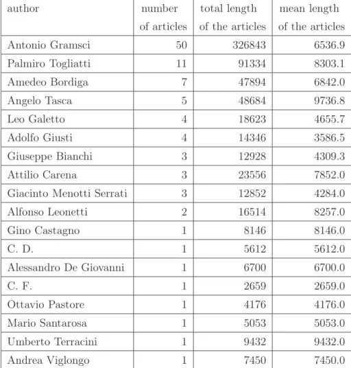
In a preliminary tuning stage we used 100 texts, 50 by Gramsci and 50 by the 17 other authors listed in Table 2.1 together with some data concerning the length of the available articles for each author. Some modifications of Kešelj’s method followed directly from the examination of the data set. First of all, we decided not to merge to a single profile all the texts of a reference author but to calculate the distance between every single pair of available texts. Indeed, in this case building the authors’ profiles as in Kešelj’s method would be in contrast with the characteristics of the 100 articles by Gramsci and coworkers, where the subdivision of the texts among the different authors is strongly heterogeneous (see Table 2.1), so that merging all texts of an author in a single profile we would have obtained profiles with very different statistical meaning: note, for example, the large disparity between the total lengths of available texts by Gramsci and by Viglongo.
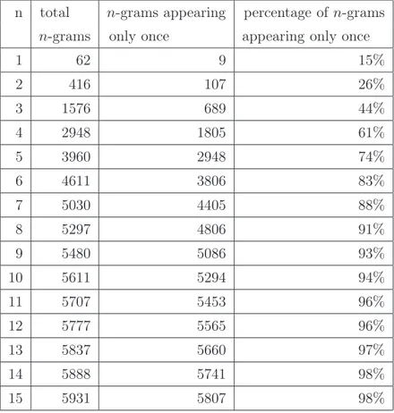
Furthermore, because of the shortness of the articles and of the choice of comparing them individually, the L parameter became unuseful and it was necessary to consider all the possible n-grams with nonzero frequency. In a single text and for large n, indeed, as can be seen from the example in Table 2.2, most of the n-grams appear just once, so that considering just the L more frequent ones would be the same as arbitrarily choosing L n-grams.
Ultimately, in order to eliminate the strong dependance of Kešelj’s for-mula on the length of the texts into consideration, the distance is divided by the sum of the number of n-grams in the two texts; the resulting formula is
the following, for two texts x, y ∈ A∗:
dn(x, y) = 1 |Dn(x)| + |Dn(y)| ! ω∈Dn(x)∪Dn(y) $ fx(ω) − fy(ω) fx(ω) + fy(ω) %2 . (2.2)
From now on we will call n-gram distance the one defined in (2.2), unless
otherwise stated. Again, dnis a pseudo-distance, since it does not satisfy the
triangular inequality and it is not even positive definite: two texts x, y can
author number total length mean length of articles of the articles of the articles Antonio Gramsci 50 326843 6536.9 Palmiro Togliatti 11 91334 8303.1 Amedeo Bordiga 7 47894 6842.0 Angelo Tasca 5 48684 9736.8 Leo Galetto 4 18623 4655.7 Adolfo Giusti 4 14346 3586.5 Giuseppe Bianchi 3 12928 4309.3 Attilio Carena 3 23556 7852.0 Giacinto Menotti Serrati 3 12852 4284.0 Alfonso Leonetti 2 16514 8257.0 Gino Castagno 1 8146 8146.0 C. D. 1 5612 5612.0 Alessandro De Giovanni 1 6700 6700.0 C. F. 1 2659 2659.0 Ottavio Pastore 1 4176 4176.0 Mario Santarosa 1 5053 5053.0 Umberto Terracini 1 9432 9432.0 Andrea Viglongo 1 7450 7450.0
Table 2.1: Total and average character length of the articles used in the
prelimi-nary phase, by author.
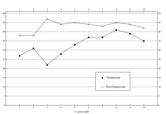
The results of the attribution of the 100 texts, obtained by assigning to each unknown text the author of its nearest neighbour according to the
distance dn, are plotted in figure 2.1. The length of n-grams varies along the
horizontal axis, with n from 1 to 10; two symbols correspond to each value of n: the circle marks the number of Gramscian texts which are correctly attributed to him by the method (true positives), while the triangle indicates the number of non-Gramscian texts which are correctly recognized as such (true negatives).
n total n-grams appearing percentage of n-grams n-grams only once appearing only once
1 62 9 15% 2 416 107 26% 3 1576 689 44% 4 2948 1805 61% 5 3960 2948 74% 6 4611 3806 83% 7 5030 4405 88% 8 5297 4806 91% 9 5480 5086 93% 10 5611 5294 94% 11 5707 5453 96% 12 5777 5565 96% 13 5837 5660 97% 14 5888 5741 98% 15 5931 5807 98%
Table 2.2: Number and percentage of occurrences of n-grams appearing only once
in the text g_27.
we achieved the best attribution results (41 texts out of 50) without loosing too much in precision (only 5 false positives). We will comment later on the implications of such a choice for n.
These first results were obtained by taking into consideration only the first neighbour of each text. Such a choice ignores the fact that the reference set contains as many as 100 different articles with which one can compare the given “unknown” text. This suggests some questions:
• what can we expect about the distance of an article by Gramsci from the 49 other texts by him?
• will these 49 articles be “nearer on the average” to the text in consid-eration?
! ! ! ! ! ! ! ! ! ! " " " " " " " " " " 1 2 3 4 5 6 7 8 9 10 0 5 10 15 20 25 30 35 40 45 50 1 2 3 4 5 6 7 8 9 10 0 5 10 15 20 25 30 35 40 45 50 n!gram length ! Gramscian " Not Gramscian
Figure 2.1: Number of correctly attributed Gramscian and non-Gramscian texts
with the first neighbour, over the 100 texts of the training corpus.
• is it possible to consider conveniently also the distances from all the other reference texts, not only the first neighbour?
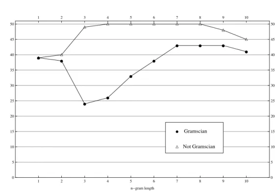
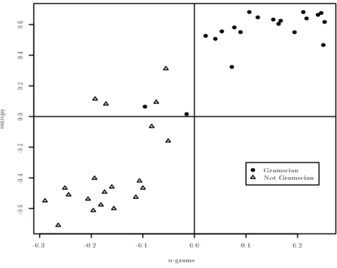
Some of these issues, especially the first, will be further discussed later, in paragraph 2.2.6. Trying to give a first answer to such questions, we defined for a text x a Gramscianity index g(x) in the following way: all the reference texts are listed in order of growing distance from the text x; the j-th text by Gramsci in the list is given the score k(j)/j, where k(j) is its rank in the list; the Gramscianity index g(x) is the sum of the scores of the 49 texts by Gramsci which appear in the list. The non-Gramscianity index ng(x) of text x is defined similarly as the sum of the corresponding scores for the first 49 texts not by Gramsci.
The Gramscianity index will be lower as long as the unknown text is nearer to the group of Gramscian texts (ng(x) has the same property for non-Gramscian texts). The text x is therefore attributed to Gramsci if its Gramscianity index g(x) is lower than its non-Gramscianity index ng(x).
! ! ! ! ! ! ! ! ! ! " " " " " " " " " " 1 2 3 4 5 6 7 8 9 10 0 5 10 15 20 25 30 35 40 45 50 1 2 3 4 5 6 7 8 9 10 0 5 10 15 20 25 30 35 40 45 50 n!gram length ! Gramscian " Not Gramscian
Figure 2.2: Attributions using Gramscianity and non-Gramscianity index, for the
100 texts of the training corpus.
Figure 2.2 illustrates, with the same conventions used for figure 2.1, the results obtained for the 100 text corpus using the index method with n-gram length from 1 to 10. Even in this case, the results suggest n = 7 or n = 8 as the best choices for the parameter; for such values, indeed, we have the best results for the recognition of texts by Gramsci (43/50 texts) and no false positive.
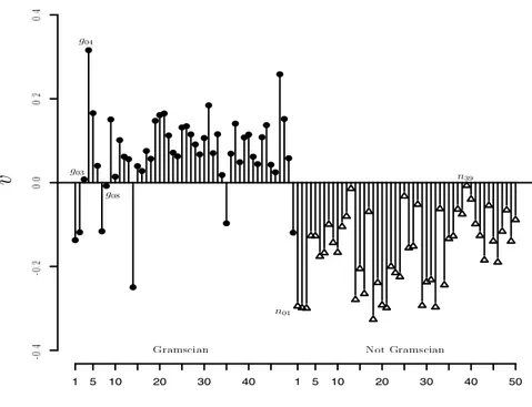
The use of these indices has also another advantage: their difference gives a natural measure of the reliability of the attribution. More precisely, given an article x to attribute, if g(x) and ng(x) are the Gramscianity and non-Gramscianity indices defined above, the number
v(x) = ng(x) − g(x)
ng(x) + g(x) (2.3)
lies always between -1 and 1: a value near to 1 (or -1) gives a strong attri-bution to Gramsci (or to “non-Gramsci”), while values near to 0 are a mark of great undecidability.
The value of the vote v for each of the 100 texts of the corpus is illustrated
in figure 2.3: it is easy to notice that some texts, for example g03, g08 and
n39, have a much weaker attribution than g04 or n01.
1 5 10 20 30 40 1 5 10 20 30 40 50 g03 g04 g08 n01 n39
v
Figure 2.3: Attribution of the 100 texts with measure of attribution reliability,
using the Gramscianity and non-Gramscianity indices defined in the text.
2.2.3
Entropy and compression: the BCL method
Shannon’s information theory, as described in chapter 1, has a rigorous and consistent formulation only for well defined mathematical objects: we have seen how the stationarity and ergodicity of the source play a fundamen-tal role in its development. Anyway, it is quite natural to use it also in the field of text analysis. Shannon himself, indeed, estimated with an experiment that the average quantity of information of the source “English language” is between 0.6 and 1.3 bits per character. Though the entropic characteristics
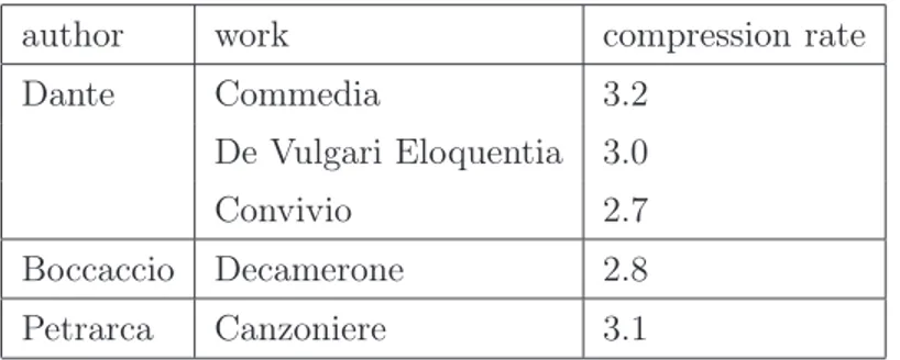
of an author’s writing are certainly interesting, an approximated value of entropy per se is not very useful for the attribution problem, as can be seen in Table 2.3, where the compression rate obtained with an LZ compressor is listed for various authors of Italian literature: it would not be possible to distinguish Dante’s works from Boccaccio’s only based on this measure and, on the other hand, different works by the same author can have very different values of entropy.
author work compression rate Dante Commedia 3.2
De Vulgari Eloquentia 3.0 Convivio 2.7 Boccaccio Decamerone 2.8 Petrarca Canzoniere 3.1
Table 2.3: Compression rates in bits per character of some texts from Italian
literature.
Moving now from a single source (author) to the comparison between two sources, relative entropy can be considered as a very powerful tool to quantify their difference: it is indeed reasonable to expect that the relative entropy of two texts by Boccaccio is smaller than the one between a text by Boccaccio and a text by Petrarca. Moreover, relative entropy can be computed effectively using compression algorithms, as we have seen in 1.
As we have seen, some compression algorithms, and the ones in the LZ family in particular, allow indeed to obtain an estimate of the relative entropy between two texts, and hence to measure their closeness. Various methods based on Ziv-Merhav’s theorem and similar ideas have been proposed and used on specific problems in the fields of biological sequence analysis and of authorship attribution; here we cite, with no pretension of completeness, the works of M. Li et al. [39], P. Juola [28], W.J. Teahan [65], O.V. Kukushkina, A.A. Polikarpov and D.V. Khmelev [35], and D. Benedetto, E. Caglioti and V. Loreto [8].