A. Ellero, A. Sorato, G. Fasano
A new model for estimating the
probability of information spreading
with opinion leaders
Working Paper n. 13/2011
November 2011
This Working Paper is published ! under the auspices of the Department of
Management at Università Ca’ Foscari Venezia. Opinions expressed herein are those
of the authors and not those of the Department or the University. The Working Paper
series is designed to divulge preliminary or incomplete work, circulated to favour
discussion and comments. Citation of this paper should consider its provisional
nature.
A New Model for Estimating the Probability of Information
Spreading with Opinion-Leaders
∗Andrea Ellero Annamaria Sorato
<[email protected]> <[email protected]>
Department of Management Department of Management
Ca’ Foscari University of Venice Ca’ Foscari University of Venice
Giovanni Fasano <[email protected]>
Department of Management Ca’ Foscari University of Venice,
INSEAN-CNR Italian Ship Model Basin
(November 2011)
Abstract. In this paper we analyze some issues related to the general problem of informa-tion spreading among individuals, where suitable assumpinforma-tions on the informainforma-tion exchange are considered. In particular, starting from the scheme proposed in [5], which is based on a majority rule to treat the individuals’ interaction, we define and introduce special indi-viduals who play a key role in the information spreading. The latter will be addressed as opinion leaders, and have the special feature of strongly interfering with the process based on the majority rule. We consider a new model, where opinion leaders are introduced as special agents, and study its specific properties which significantly recast some conclusions worth for the model in [5]. Finally, we provide some results cocerning the dynamics of the model.
Keywords: Information spreading, Galam’s model, Opinion leaders. JEL Classification Numbers: C02, C40.
Correspondence to:
Andrea Ellero Department of Management, Ca’ Foscari University of Venice San Giobbe, Cannaregio 873
30121 Venice, Italy Phone: [+39] 041-234-6930 Fax: [+39] 041-234-7444 E-mail: [email protected]
1
Introduction
Diffusion dynamics applied to social sciences has been studied in a huge number of papers and books, covering a wide range of perspectives, from marketing (see e.g. [1], [13], [12]) to agent based modeling (see e.g. [14], [9]) and sociophysics [5].
The point of view adopted in this paper is based on a model proposed by Galam for information spreading among agents of a population [5]. In this model the agents can have one of two opposite opinions and each of them has the same impact on the others’ opinion by means of repeated discussions in subgroups. In our proposal we suitably recast Galam’s model, in order to introduce “opinion-leader” agents, who can drive the opinion of the agents joining the same discussion group.
The interest in opinion leaders has been increasing in recent years due to the exponential growth of social networks and the Web 2.0, since a small group of opinion leaders may accelerate, or even stop, information spreading, especially in the initial phase of the process. In fact, as originally observed by [11], some members of a social network are “likely to influence other persons in their immediate environment” and enhance diffusion processes. They affect the spreading of information or the diffusion and adoption of a new product through different communication channels. In the literature, opinion leaders are also called influentials, mavens, hubs, and they are convincing experts, or have a large number of social ties [15], [10], [16], [3].
The opinion leaders we consider in our models are able to convince all the agents they meet in a discussion group and keep their opinion forever. We both provide theoretical motivations to justify our proposal, and preliminary results which carry out the role of opinion-leaders. In particular, we focus on their effectiveness in modifying the dynamics of information spreading.
This paper is organized as follows: Section 2 partially reviews Galam’s model [5], de-tailing some of its peculiarities along with possible limits. Then, in Section 3 we describe some preliminaries to our model, including the definition of opinion leaders, which is es-sential to our analysis. Section 4 is devoted to report some properties of our model, and Section 5 includes a comparative analysis of the dynamics of the model. Finally, a section of Conclusions completes the paper, along with an Appendix of basic key-note results.
2
The original Galam’s model
This section briefly reviews Galam’s model in [5], [6], along with some of its features. In order to introduce the latter model we preliminarily consider the following process. There are 𝑁 independent individuals (agents) who synchronize their behaviour and periodically meet into subsets (say subgroups) of individuals. Each subgroup, at period 𝑡 ≥ 1, has cardinality 𝑘, with 𝑘 ranging from 1 to 𝐿, being 𝐿 a positive integer. Each individual either thinks ‘+’ or ‘−’, and 𝑁+(𝑡) [𝑁−(𝑡)] corresponds to the overall number of people thinking
+ [−] at period 𝑡, among the 𝑁 individuals. Thus, we have the consistency relation 𝑁 = 𝑁+(𝑡) + 𝑁−(𝑡), ∀𝑡 = 1, 2, . . .
Observe that at period 𝑡, with 𝑡 ≥ 1, there may be in general several subgroups of size 𝑘, with 1 ≤ 𝑘 ≤ 𝐿. At period 𝑡, with probability 𝑎𝑘, 𝑘 = 1, . . . , 𝐿, the 𝑁 people gather into
𝑘-sized subgroups; thus, again for consistency reasons, the relation
𝐿
∑
𝑘=1
𝑎𝑘= 1, 𝑎𝑘 ≥ 0, 𝑘 = 1, . . . , 𝐿 (1)
trivially holds. Then, at the outset of the following period 𝑡 + 1, after a discussion in each 𝑘-sized subgroup, each individual can reverse their opinion to the opposite one (say ‘+’ becomes ‘−’ or viceversa), according with a majority rule (in each subgroup). The rule for reversing opinion is slightly biased in favor of the opinion ‘−’, since in case of parity in a subgroup ‘−’ will prevail over ‘+’. In symbols, if 𝑁𝑘ℎ
+ (𝑡) [𝑁𝑘
ℎ
− (𝑡)] denotes the number of
individuals thinking ‘+’ [‘−’] at period 𝑡 in the ℎ-th subgroup of size 𝑘, then1 ∙ if 𝑁𝑘ℎ
+ (𝑡) > 𝑁𝑘
ℎ
− (𝑡) then at the outset of the period 𝑡 + 1 the 𝑁 𝑘ℎ
− (𝑡) individuals’
opinion will reverse from ‘−’ to ‘+’; ∙ if 𝑁𝑘ℎ
+ (𝑡) ≤ 𝑁𝑘
ℎ
− (𝑡) then at the outset of the period 𝑡 + 1 the 𝑁 𝑘ℎ
+ (𝑡) individuals’
opinion will reverse from ‘+’ to ‘−’.
We respectively indicate with 𝑃+(𝑡) [𝑃−(𝑡)] the ‘estimated’ probability, at period ‘𝑡’, to find
individuals who think ‘+’ [‘−’] among the 𝑁 individuals. Thus, for any 𝑡 ≥ 1 the quantity 𝑃+(𝑡) [𝑃−(𝑡)] may possibly differ from the ‘actual’ value of the probability ˜𝑃+(𝑡)[ ˜𝑃−(𝑡)] to
find individuals thinking ‘+’ [‘−’] among the 𝑁 individuals, the latter being ˜ 𝑃+(𝑡) = 𝑁+(𝑡) 𝑁 ˜ 𝑃−(𝑡) = 𝑁−(𝑡) 𝑁 with ˜ 𝑃−(𝑡) + ˜𝑃+(𝑡) = 1.
Then, given the parameters 𝐿 and 𝑎1, . . . , 𝑎𝐿, and the quantity 𝑃+(𝑡), Galam’s model
may be recursively used to estimate the probability 𝑃+(𝑡 + 1) of having individuals thinking
‘+’ at period 𝑡 + 1, using the formula 𝑃+(𝑡 + 1) = 𝐿 ∑ 𝑘=1 𝑎𝑘 𝑘 ∑ 𝑗=⌊𝑘 2+1⌋ 𝐶𝑗𝑘𝑃+(𝑡)𝑗{1 − 𝑃+(𝑡)}𝑘−𝑗. (2)
Note that in (2) the quantity ⌊𝑧⌋ indicates the largest integer which approximates 𝑧 from below, and 𝐶𝑘
𝑗 is the binomial coefficient
𝐶𝑗𝑘 = 𝑘!
𝑗!(𝑘 − 𝑗)!, 𝑘 = 1, . . . , 𝐿, 𝑗 ≤ 𝑘.
Moreover, due to a natural consistency reason we set ˜𝑃+(0) = 𝑃+(0) and ˜𝑃−(0) = 𝑃−(0).
Now, following the observations in [5] and [4], we can represent the recursive expression (2) in the space (𝑃+(𝑡), 𝑃+(𝑡 + 1)), so that the special point ( ˆ𝑃+, ˆ𝑃+) in the resulting graph
may be appointed (namely the killing point), satisfying the conditions
1
Note that with an obvious use of the symbols we have∑𝐿𝑘=1
∑ ℎ𝑁 𝑘ℎ + (𝑡) = 𝑁+(𝑡) and∑ 𝐿 𝑘=1 ∑ ℎ𝑁 𝑘ℎ − (𝑡) = 𝑁 −(𝑡). 2
if 𝑃+(0) > ˆ𝑃+ then lim
𝑡→∞𝑃+(𝑡) = 1,
if 𝑃+(0) = ˆ𝑃+ then 𝑃+(0) = 𝑃+(𝑡), for each period 𝑡 > 0,
if 𝑃+(0) < ˆ𝑃+ then lim
𝑡→∞𝑃+(𝑡) = 0.
In the next Section we are going to propose and study the introduction of special individuals among the 𝑁 members of the group.
3
A new perspective introducing Opinion Leaders
We consider now the special individuals called opinion leaders. In order to study their effect on the information spreading process defined by Galam, we modify formula (2). We need to introduce the following preliminary definition of opinion leaders.
Definition 3.1 Suppose that at the outset of the period 𝑡, when the agents gather into subgroups, the 𝑘 agents 𝑖1(𝑡), . . . , 𝑖𝑘(𝑡) form the 𝑘-sized subgroup 𝐺𝑘(𝑡). Then agent 𝑗 in
𝐺𝑘(𝑡) is said to be an op-leader (opinion leader) if
1. 𝑗 always thinks ‘+’, for any 𝑡 ≥ 1;
2. at the end of the period 𝑡 all agents of the subgroup 𝐺𝑘(𝑡) think ‘+’.
Broadly speaking an op-leader is one of the individuals thinking ‘+’ for any 𝑡 ≥ 1 who is able to convince all the other individuals in a subgroup to think ‘+’. Thus, from Definition 3.1 the role of the op-leaders we have just introduced partially summarizes some informal definitions given in the literature.
Similarly to the original Galam’s model in (2), given the parameters 𝐿 and 𝑎1, . . . , 𝑎𝐿,
along with the quantity 𝑃+(𝑡) and the number of op-leaders 𝑁𝑜𝑝, we want to estimate the
probability 𝑃+(𝑡 + 1) of having individuals thinking ‘+’ at period 𝑡 + 1. With this aim we
propose the following model
𝑃+(𝑡 + 1) = 1 − 𝐿 ∑ 𝑘=1 𝑎𝑘 ⌊𝑘 2⌋ ∑ 𝑗=0 𝐶𝑗𝑘{𝑃+(𝑡) − 𝑠}𝑗{1 − 𝑃+(𝑡)}𝑘−𝑗 (3)
where 𝑠 is the probability for an agent to be an op-leader.
The quantity {𝑃+(𝑡) − 𝑠}𝑗{1 − 𝑃+(𝑡)}𝑘−𝑗 approximates the probability that in a
𝑘-sized subgroup 𝑗 individuals think ‘+’ without being op-leaders and the remaining 𝑘 − 𝑗 individuals think ‘−’. Since we consider the majority rule also adopted in Galam’s model, the quantity∑⌊
𝑘 2⌋
𝑗=0 𝐶𝑗𝑘{𝑃+(𝑡) − 𝑠}𝑗{1 − 𝑃+(𝑡)}𝑘−𝑗 in (3) approximates the probability that
an individual of a 𝑘-sized subgroup will think ‘−’ at the end of period 𝑡.
We observe that model (3) considers three independent events: ‘the agent thinks + without being an op-leader’, ‘the agent thinks −’ and ‘the agent is an op-leader’. This implies that the model (3) is based on a more general trinomial distribution where the probability to have, in a group of size 𝑘, 𝑗 ‘+ agents (not op-leader)’, ℎ ‘op-leaders’ and 𝑘 − 𝑗 − ℎ ‘− agents’ is:
The probability (4) reduces to
𝐶𝑗𝑘{𝑃+(𝑡) − 𝑠}𝑗{1 − 𝑃+(𝑡)}𝑘−𝑗 (5)
since in our special case, ℎ = 0.
4
Preliminary properties
In this section some theoretical properties of (2) and (3) are partially described.
Proposition 4.1 Consider relation (3) with 𝑎𝐿 = 1, 𝑠 = 0 and where 𝐿 is odd. Then (3)
coincides with (2) and we have for any 𝑡 ≥ 1 𝑃+(𝑡) =
1
2 =⇒ 𝑃+(𝑡 + 1) = 𝑃+(𝑡). (6)
Proof
When 𝑠 = 0, since 𝑃+(𝑡) = 1/2 then for any 𝑗
{𝑃+(𝑡)}𝑗{1 − 𝑃+(𝑡)}𝐿−𝑗 =
1 2𝐿.
Moreover, since 𝐿 is odd, the binomial theorem yields
𝐿 ∑ 𝑗=0 𝐶𝑗𝐿= 2𝐿, ⌊𝐿 2⌋ ∑ 𝑗=0 𝐶𝑗𝐿= 2𝐿−1. Therefore, 𝑃+(𝑡 + 1) = 1/2. □
Remark 4.1 Observe that also in case 𝐿 is even and the majority rule holds, without a bias for ‘−’, i.e. in case of parity, the two opinions have the same probability to prevail, then a result similar to Proposition 4.1 holds.
Further properties on the computation of the killing point, for some special values of 𝐿 may be found in Section 7.
5
Dynamics of the model
In this section we consider some properties of the dynamics of the model also in order to compare it with the original Galam’s model (2). On this purpose, suppose we indicate with 𝒫𝐿 the function
𝑃+(𝑡 + 1) = 𝒫𝐿(𝑃+(𝑡))
of 𝑃+(𝑡 + 1) vs. 𝑃+(𝑡) as defined in model (2), and let be 𝒫𝑚𝐿 the function 𝒫𝐿 where we
set 𝑎𝑘= 0, for any 𝑘 ∕= 𝑚, 1 ≤ 𝑚 ≤ 𝐿, and 𝑎𝑚= 1. Then, from (2) we immediately realize
that
Property 5.1 Let us consider the nonnegative coefficients 𝑎𝑘, 𝑘 = 1, . . . , 𝐿, such that (1)
holds. Then, the function 𝒫𝐿 is given by the weighted sum
𝒫𝐿= 𝐿 ∑ 𝑘=1 𝑎𝑘𝒫𝑘𝐿. 4
Thus, in order to study some of the general properties of (2) and (3) it might suffice to consider what happens setting 𝑎𝑘 = 0, for any 𝑘 ∕= 𝑚, 1 ≤ 𝑚 ≤ 𝐿, and 𝑎𝑚 = 1. To this
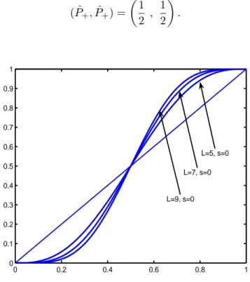
end, we preliminarily give in Figure 1 the graphs of 𝑃+(𝑡 + 1) vs. 𝑃+(𝑡), as described by (2)
(or equivalently setting 𝑠 = 0 in (3)), choosing respectively 𝑚 ∈ {5, 7, 9} (i.e., values for 𝑚 which are in a set of odd indices). Recalling Property 5.1 and Proposition 4.1, from Figure 1 we deduce the following result.
Property 5.2 In case in (2) we have 𝑎𝑘 = 0, for any even 𝑘, with 1 ≤ 𝑘 ≤ 𝐿, then the
function 𝒫𝐿 has the killing point
( ˆ𝑃+, ˆ𝑃+) = ( 1 2 , 1 2 ) . 0 0.2 0.4 0.6 0.8 1 0 0.1 0.2 0.3 0.4 0.5 0.6 0.7 0.8 0.9 1 L=5, s=0 L=7, s=0 L=9, s=0
Figure 1: Galam’s formula (2) with 𝑎𝑘 = 0, for any 𝑘 ∕= 𝐿, and 𝐿 ∈ {5, 7, 9} (with no
op-leader, i.e. 𝑠 = 0). Since 𝐿 is ‘odd’, in all the three cases the killing point is always (1/2, 1/2).
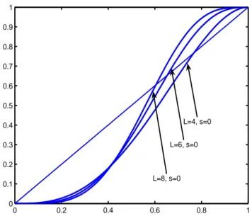
The same result of course does not hold if 𝑎𝑘∕= 0, for some even 𝑘, 1 ≤ 𝑘 ≤ 𝐿. An example
is given in Figure 2, where we respectively set 𝑚 ∈ {4, 6, 8} in (2). Observe that due to the bias of the majority rule in favor of ‘−’, the killing point when 𝑚 is even must be not smaller than 1/2. In particular, from Figure 2 and using the Property 5.1, we deduce that the killing point of the graph 𝒫𝐿 is bounded from below by 1/2 and bounded from above by the killing point of 𝒫𝐿
𝑝, where
𝑝 = min
1≤𝑖≤𝐿{𝑖 : 𝑖 is even and 𝑎𝑖 ∕= 0}.
Therefore, if 𝑎2 = 0 then (1 +√13)/6 is an upper bound for the killing point, as proved in
Section 7 (see also [2])2.
2
0 0.2 0.4 0.6 0.8 1 0 0.1 0.2 0.3 0.4 0.5 0.6 0.7 0.8 0.9 1 L=4, s=0 L=6, s=0 L=8, s=0
Figure 2: Galam’s formula (2) with 𝑎𝑘 = 0, for any 𝑘 ∕= 𝐿, and 𝐿 ∈ {4, 6, 8} (with no
op-leader, i.e. 𝑠 = 0). Since 𝐿 is ‘even’, in all the three cases the killing point differs from (1/2, 1/2) and we always have ˆ𝑃+> 1/2.
From Figures 1-2 there is an empirical evidence that when 𝑃+(𝑡) > 1/2 then 𝑃+(𝑡 + 1)
increases with 𝐿.
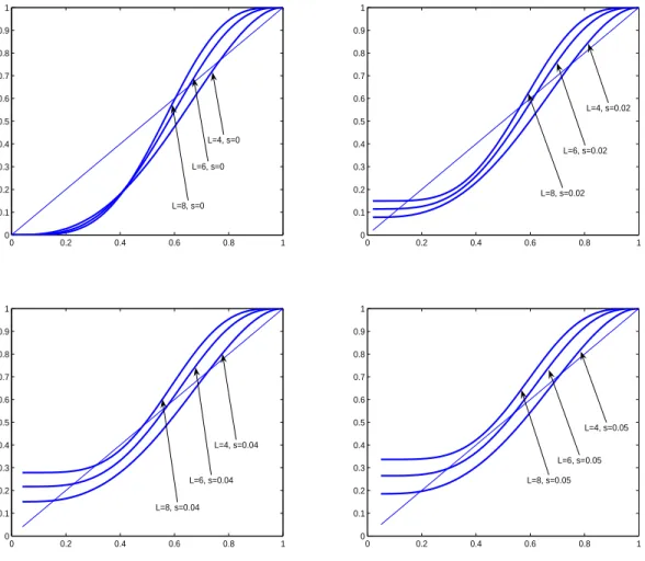
Now we consider the case in which the formula (3) is used, in place of (2), and nonzero values of the parameter 𝑠 are selected. We want to use the same setting of the parameters 𝐿 and 𝑎𝑘, 1 ≤ 𝑘 ≤ 𝐿, used for the Figures 1-2. Moreover, recalling that when 𝑠 = 0 the
equations (3) and (2) coincide, the Figure 3 (𝐿 is odd with 𝐿 ∈ {5, 7, 9}) and Figure 4 (𝐿 is even with 𝐿 ∈ {4, 6, 8}) show the graph of 𝑃+(𝑡 + 1) vs. 𝑃+(𝑡) when 𝑠 ∈ {0, 0.02, 0.04, 0.05}
(i.e., when no op-leader is included and when the probability of having op-leaders is respec-tively raised to 2%, 4% and 5%). Observe that in the pictures where 𝑠 ∕= 0, from (3) we do have to consider for 𝑃+(𝑡) values such that 𝑃+(𝑡) > 𝑠. This explains why the latter graphs
are not defined for 𝑃+(𝑡) < 𝑠. Also note that in (4), where 𝐿 is even, the killing point
progressively decreases and approaches ˆ𝑃+ = 1/2 when 𝑠 increases.
Observe that in case 𝑠 = 0 (see (2) and Section 7.1), then 𝑃+(𝑡+1) = 𝑃+(𝑡) if 𝑃+(𝑡) = 0.
On the contrary, from Figures 3-4 it seems that in case 𝑠 ∕= 0 then 𝑃+(𝑡 + 1) = 𝑃+(𝑡) only
if 𝑃+(𝑡) > 0 (which recalls some similar results in [7]).
Interestingly enough, the observation of Figures 3-4 reveals also that there is a threshold value for 𝑠 such that the graph of 𝑃+(𝑡+1) vs. 𝑃+(𝑡) becomes tangent to the line 𝑃+(𝑡+1) =
𝑃+(𝑡), above that threshold the killing point is ˆ𝑃+= 1, regardless of the choice of the initial
value 𝑃+(0). The latter observation deserves a special attention, also considering the large
number of applications where it could be fruitfully recast.
Finally, the effect of op-leaders appears to be clearly more evident when 𝐿 is large, i.e. when the discussions take place in large groups.
0 0.2 0.4 0.6 0.8 1 0 0.1 0.2 0.3 0.4 0.5 0.6 0.7 0.8 0.9 1 L=5, s=0 L=7, s=0 L=9, s=0 0 0.2 0.4 0.6 0.8 1 0 0.1 0.2 0.3 0.4 0.5 0.6 0.7 0.8 0.9 1 L=5, s=0.02 L=7, s=0.02 L=9, s=0.02 0 0.2 0.4 0.6 0.8 1 0 0.1 0.2 0.3 0.4 0.5 0.6 0.7 0.8 0.9 1 L=5, s=0.04 L=7, s=0.04 L=9, s=0.04 0 0.2 0.4 0.6 0.8 1 0 0.1 0.2 0.3 0.4 0.5 0.6 0.7 0.8 0.9 1 L=7, s=0.05 L=5, s=0.05 L=9, s=0.05
Figure 3: Our proposal (3) where the values of 𝐿 and 𝑠 are given. Again, as in Figures 1-2, we have 𝑎𝑘= 0, for any 𝑘 ∕= 𝐿. Here 𝐿 is ‘odd’, being 𝐿 ∈ {5, 7, 9}. The effect of op-leaders
is more evident when 𝐿 is large.
6
Conclusions
This paper was devoted to preliminarily analyze some properties of Galam’s model [5], along with introducing a new model for information spreading. In particular, the novelty of the contribution of this paper consists of addressing special individuals, namely opinion leaders, and their keynote role in information spreading, when the majority rule defined in [5] holds.
We have described the novel models along with a few properties of them, and a partial numerical experience. We think that in a broad sense a complete and motivated analysis is yet mandatory, in order to carefully assess further properties and limits of our proposals. Also possible generalizations of the model to the spreading of more than two opinions in the populations could be developed (see also [8]).
0 0.2 0.4 0.6 0.8 1 0 0.1 0.2 0.3 0.4 0.5 0.6 0.7 0.8 0.9 1 L=4, s=0 L=6, s=0 L=8, s=0 0 0.2 0.4 0.6 0.8 1 0 0.1 0.2 0.3 0.4 0.5 0.6 0.7 0.8 0.9 1 L=4, s=0.02 L=6, s=0.02 L=8, s=0.02 0 0.2 0.4 0.6 0.8 1 0 0.1 0.2 0.3 0.4 0.5 0.6 0.7 0.8 0.9 1 L=4, s=0.04 L=6, s=0.04 L=8, s=0.04 0 0.2 0.4 0.6 0.8 1 0 0.1 0.2 0.3 0.4 0.5 0.6 0.7 0.8 0.9 1 L=4, s=0.05 L=6, s=0.05 L=8, s=0.05
Figure 4: Our proposal (3) where the values of 𝐿 and 𝑠 are given. Again, as in Figures 1-2, we have 𝑎𝑘 = 0, for any 𝑘 ∕= 𝐿. Here 𝐿 is ‘even’, being 𝐿 ∈ {4, 6, 8}. The effect of
op-leaders is more evident when 𝐿 is large.
7
Appendix (some properties of (2))
Let us consider the following expression from the binomial theorem (1 − 𝑥)𝑘−𝑗 = 𝑘−𝑗 ∑ ℎ=0 ( 𝑘 − 𝑗 ℎ ) 1ℎ(−𝑥)𝑘−𝑗−ℎ = 𝑘−𝑗 ∑ ℎ=0 ( 𝑘 − 𝑗 ℎ ) (−1)𝑘−𝑗−ℎ𝑥𝑘−𝑗−ℎ. 8
Hence, from (2) we have 𝑃+(𝑡 + 1) = 𝐿 ∑ 𝑘=1 𝑎𝑘 𝑘 ∑ 𝑗=⌊𝑘 2+1⌋ 𝐶𝑗𝑘𝑃+(𝑡)𝑗{1 − 𝑃+(𝑡)}𝑘−𝑗 (7) = 𝐿 ∑ 𝑘=1 𝑎𝑘 𝑘 ∑ 𝑗=⌊𝑘 2+1⌋ 𝑘−𝑗 ∑ ℎ=0 ( 𝑘 𝑗 ) ( 𝑘 − 𝑗 ℎ ) (−1)𝑘−𝑗−ℎ𝑃+(𝑡)𝑘−𝑗−ℎ+𝑗 = 𝐿 ∑ 𝑘=1 𝑎𝑘 𝑘 ∑ 𝑗=⌊𝑘 2+1⌋ 𝑘−𝑗 ∑ ℎ=0 (−1)𝑘−𝑗−ℎ ( 𝑘 𝑗 ) ( 𝑘 − 𝑗 ℎ ) 𝑃+(𝑡)𝑘−ℎ = 𝐿 ∑ 𝑘=1 𝑘 ∑ 𝑗=⌊𝑘2+1⌋ 𝑘−𝑗 ∑ ℎ=0 (−1)𝑘−𝑗−ℎ𝑎𝑘 ( 𝑘 𝑗 ) ( 𝑘 − 𝑗 ℎ ) 𝑃+(𝑡)𝑘−ℎ (8)
Proposition 7.1 Consider relation (7), where 𝐿 is a positive integer and ∑𝐿
𝑘=1𝑎𝑘 = 1,
with 𝑎𝑘 ≥ 0, 𝑘 = 1, . . . , 𝐿. For any choice of 𝑃+(𝑡) ∈ [0, 1] and any choice of 𝐿, we have
𝑃+(𝑡 + 1) = 𝑃+(𝑡) if and only if
𝑎1 = 1
𝑎𝑘 = 0, 𝑘 = 2, . . . , 𝐿. (9)
Furthermore, considering (7) and (8), for any 𝐿 ≥ 1 the expression 𝑃+(𝑡) = 𝐿 ∑ 𝑘=1 𝑘 ∑ 𝑗=⌊𝑘 2+1⌋ 𝑘−𝑗 ∑ ℎ=0 (−1)𝑘−𝑗−ℎ𝑎𝑘 ( 𝑘 𝑗 ) ( 𝑘 − 𝑗 ℎ ) 𝑃+(𝑡)𝑘−ℎ (10)
admits the solutions 𝑃+(𝑡) = 0 (for any 𝐿 ≥ 1) and 𝑃+(𝑡) = 1 (for any 𝐿 ≥ 2).
Proof
The sufficient condition is self-evident since (9) implies that 𝑃+(𝑡 + 1) = 𝑃+(𝑡), for any
choice of the parameter 𝐿 in (7). On the other hand, the necessary condition follows from the fact that (8) must hold for any value of the integer 𝐿.
Finally, equation (10) is homogeneous with respect to 𝑃+(𝑡) so that 𝑃+(𝑡) = 0 is clearly
a solution. In addition, since in (7)
lim 𝑃+(𝑡)→1 {1 − 𝑃+(𝑡)}𝑘−𝑗 = ⎧ ⎨ ⎩ 0 if 𝑘 ∕= 𝑗 1 if 𝑘 = 𝑗, we have lim 𝑃+(𝑡)→1 𝐿 ∑ 𝑘=1 𝑎𝑘 𝑘 ∑ 𝑗=⌊𝑘 2+1⌋ 𝐶𝑗𝑘𝑃+(𝑡)𝑗{1 − 𝑃+(𝑡)}𝑘−𝑗 = 𝑃+(𝑡),
which proves that 𝑃+(𝑡) = 1 is again a solution of (10). □.
Now, we want preliminarily to compute the killing point in the case where the model (7) is used and 𝐿 = 1, . . . , 4; then, we will have to extend the results to our proposals. The cases where 𝐿 = 1, . . . , 4 are important since several practical problems, where small groups
of individuals are involved, are pretty common.
Let us examine the trivial case 𝐿 = 1. This implies that the subsets of people may have just one member; thus, each of the 𝑁 individuals will preserve their initial opinion. The killing point corresponds to ˆ𝑃+= 1 and the conclusions of Proposition 7.1 clearly hold.
Let now be 𝐿 = 2 (the dance hall problem). According with (8) with 𝐿 = 2 we have 𝑃+(𝑡 + 1) = 1 ∑ 𝑗=⌊1 2+1⌋ 1−𝑗 ∑ ℎ=0 (−1)1−𝑗−ℎ𝑎1 ( 1 𝑗 ) ( 1 − 𝑗 ℎ ) 𝑃+(𝑡)1−ℎ + 2 ∑ 𝑗=⌊2 2+1⌋ 2−𝑗 ∑ ℎ=0 (−1)2−𝑗−ℎ𝑎2 ( 2 𝑗 ) ( 2 − 𝑗 ℎ ) 𝑃+(𝑡)2−ℎ = 𝑎1𝑃+(𝑡) + 𝑎2𝑃+(𝑡)2.
The killing point may be determined using relation∑𝐿
𝑖=0𝑎𝑘= 1 and by solving the equation
𝑃+(𝑡) = 𝑎1𝑃+(𝑡) + 𝑎2𝑃+(𝑡)2.
If 𝑎2 = 0 we fall in the previous case where 𝐿 = 1. Otherwise, from Proposition 7.1 we have
the two stationary points ‘0’ and ‘1’, where only ‘1’ is the killing point ˆ𝑃+.
When 𝐿 = 3 we have to consider the cases 𝑘 = 1, 2, 3. Thus, (8) becomes 𝑃+(𝑡 + 1) = 1 ∑ 𝑗=⌊1 2+1⌋ 1−𝑗 ∑ ℎ=0 (−1)1−𝑗−ℎ𝑎1 ( 1 𝑗 ) ( 1 − 𝑗 ℎ ) 𝑃+(𝑡)1−ℎ + 2 ∑ 𝑗=⌊2 2+1⌋ 2−𝑗 ∑ ℎ=0 (−1)2−𝑗−ℎ𝑎2 ( 2 𝑗 ) ( 2 − 𝑗 ℎ ) 𝑃+(𝑡)2−ℎ + 3 ∑ 𝑗=⌊3 2+1⌋ 3−𝑗 ∑ ℎ=0 (−1)3−𝑗−ℎ𝑎3 ( 3 𝑗 ) ( 3 − 𝑗 ℎ ) 𝑃+(𝑡)3−ℎ = 𝑎1𝑃+(𝑡) + 𝑎2𝑃+(𝑡)2− 3𝑎3𝑃+(𝑡)3+ 3𝑎3𝑃+(𝑡)2+ 𝑎3𝑃+(𝑡)3 = 𝑎1𝑃+(𝑡) + (𝑎2+ 3𝑎3)𝑃+(𝑡)2− 2𝑎3𝑃+(𝑡)3.
As Proposition 7.1 stated, from equation (10) we see that 𝑃+(𝑡) = 0, for any 𝑡 ≥ 0, is a
solution. Furthermore, the other two solutions of (10) are given by (the case 𝑎3= 0 simply
yields the same results of 𝐿 = 2) 1 4𝑎3 [ 𝑎2+ 3𝑎3+ (𝑎23− 2𝑎2𝑎3+ 𝑎22)1/2 ] = 1 4𝑎3 [𝑎2+ 3𝑎3+ (𝑎3− 𝑎2)] = 1 1 4𝑎3 [ 𝑎2+ 3𝑎3− (𝑎23− 2𝑎2𝑎3+ 𝑎22)1/2 ] = 1 4𝑎3 [𝑎2+ 3𝑎3− (𝑎3− 𝑎2)] = 𝑎2+ 𝑎3 2𝑎3 ≥ 1 2. The latter formulae confirm two obvious considerations. First, the results of Proposition 7.1 hold. Then, in case the majority rule is adopted within each subset of individuals (with
a bias for ‘−’ in case of ties), then the killing point ˆ𝑃+= (𝑎2+ 𝑎3)/(2𝑎3) is larger than 0.5.
Note also that in case 𝑎1 = 𝑎2 = 0 the results of Proposition 4.1 trivially hold.
When 𝐿 = 4 we have the cases 𝑘 = 1, 2, 3, 4. Thus, (8) becomes
𝑃+(𝑡 + 1) = 1 ∑ 𝑗=⌊1 2+1⌋ 1−𝑗 ∑ ℎ=0 (−1)1−𝑗−ℎ𝑎1 ( 1 𝑗 ) ( 1 − 𝑗 ℎ ) 𝑃+(𝑡)1−ℎ + 2 ∑ 𝑗=⌊2 2+1⌋ 2−𝑗 ∑ ℎ=0 (−1)2−𝑗−ℎ𝑎2 ( 2 𝑗 ) ( 2 − 𝑗 ℎ ) 𝑃+(𝑡)2−ℎ + 3 ∑ 𝑗=⌊3 2+1⌋ 3−𝑗 ∑ ℎ=0 (−1)3−𝑗−ℎ𝑎3 ( 3 𝑗 ) ( 3 − 𝑗 ℎ ) 𝑃+(𝑡)3−ℎ + 4 ∑ 𝑗=⌊4 2+1⌋ 4−𝑗 ∑ ℎ=0 (−1)4−𝑗−ℎ𝑎4 ( 4 𝑗 ) ( 4 − 𝑗 ℎ ) 𝑃+(𝑡)4−ℎ = 𝑎1𝑃+(𝑡) + (𝑎2+ 3𝑎3)𝑃+(𝑡)2+ (4𝑎4− 2𝑎3)𝑃+(𝑡)3− 3𝑎4𝑃+(𝑡)4.
In order to compute possible killing points for the case 𝐿 = 4 we consider the solution of equation
𝑃+(𝑡) = 𝑎1𝑃+(𝑡) + (𝑎2+ 3𝑎3)𝑃+(𝑡)2+ (4𝑎4− 2𝑎3)𝑃+(𝑡)3− 3𝑎4𝑃+(𝑡)4
and equivalently
(𝑎1− 1)𝑃+(𝑡) + (𝑎2+ 3𝑎3)𝑃+(𝑡)2+ (4𝑎4− 2𝑎3)𝑃+(𝑡)3− 3𝑎4𝑃+(𝑡)4 = 0.
Again from Proposition 7.1 and equation (10) we see that 𝑃+(𝑡) = 0, for any 𝑡 ≥ 0, is
a solution. Furthermore, since also 𝑃+(𝑡) = 1 must be a solution of (10) by a simple
polynomial division we obtain
(𝑎1− 1)𝑃+(𝑡) + (𝑎2+ 3𝑎3)𝑃+(𝑡)2+ (4𝑎4− 2𝑎3)𝑃+(𝑡)3− 3𝑎4𝑃+(𝑡)4 =
𝑃+(𝑡) [𝑃+(𝑡) − 1][3𝑎4𝑃+(𝑡)2+ (2𝑎3− 𝑎4)𝑃+(𝑡) + (𝑎1− 1)] ,
so that the zeros (possible killing points) are 1 6𝑎4 [ 𝑎4− 2𝑎3+ ((2𝑎4+ 2𝑎3)2+ 3𝑎4(3𝑎4+ 4𝑎2))1/2 ] > 4𝑎4 6𝑎4 = 2 3 1 6𝑎4 [ 𝑎4− 2𝑎3− ((2𝑎4+ 2𝑎3)2+ 3𝑎4(3𝑎4+ 4𝑎2))1/2 ] < 0. (11)
Then, in case the majority rule is adopted within each subset of individuals (with a bias for ‘−’ in case of ties), the left hand side of (11) is negative and therefore cannot be a killing point.
Moreover, also observe that in case 𝑎4 = 1 (i.e. only subgroups with four individuals are
References
[1] Bass, F., A new product growth model for consumer durables, Management Science 15,5 (1969) 215-227.
[2] Bouzdine-Chameeva, T. and Galam, S. Word-of-mouth versus experts and reputation in the individual dynamics of wine purchasing, Advances in Complex Systems, 14, 6 (2011) 1–15.
[3] Cho, Y., Hwang, J. and Lee, D., Identification of effective opinion leaders in the diffu-sion of technological innovation: A social network approach Technological Forecasting and Social Change (2011), In Press, doi:10.1016/J.Techfore.2011.06.003.
[4] Ellero, A., Fasano, G. and Sorato, A., A Modified Galam’s Model for Word-of-Mouth Information Exchange, Physica A: Statistical Mechanics and its Applications, 388, 18 (2009) 3901–3910.
[5] Galam, S., Modelling rumors: the no plane Pentagon French hoax case, Physica A 320 (2003) 571–580.
[6] Galam, S., Sociophysics: a review of Galam models, International Journal of Modern Physics C 19-3 (2008) 409-440.
[7] Galam, S., and Jacobs, F., The role of inflexible minorities in the breaking of democratic opinion dynamics, Physica A 381 (2007) 366–376.
[8] Gekle, S., Peliti, L. and Galam S., Opinion dynamics in three-choice system, European Physics Journal B 45 (2005) 569–575.
[9] Garber, T., Goldenberg, J., Libai, B., and Muller E., From density to destiny: using spatial dimension of sales data for early prediction of new product success, Marketing Science 23 (2004) 419–428.
[10] Goldenberg, J., Han, S., Lehmann, D.R. and Hong J.W., The Role of Hubs in the Adoption Processes Journal of Marketing 73-2 (2009) 1–13.
[11] Katz, E., Lazarsfeld, P. F., Personal influence: The part played by people in the flow of mass communication Glencoe, IL, Free Press, 1955.
[12] Moore, G.A., Crossing the chasm, Harper Business, New York, 1991.
[13] Rogers, E., M., Diffusion of Innovations, 5th ed., New York, Free Press, 2003.
[14] Schelling, T.C., Dynamic Models of Segregation Journal of Mathematical Sociology 1 (1971) 143–186.
[15] van Eck, P. S., Jager, W. and Leeflang, P.S.H., Opinion Leaders’ Role in Innovation Diffusion: A Simulation Study Journal of Product Innovation Management 28 (2011) 187-203.
[16] Watts, D., Dodds, P.S.,Influentials, networks and public opinion formation Journal of Consumer Research 34 (2007) 441–458.