Flood Routing Efficiency Assessment: an
Approach Using Bivariate Copulas
Matteo Balistrocchi
1*†, Roberto Ranzi
1, Stefano Orlandini
2and
Baldassare Bacchi
11 University of Brescia, Brescia, IT
2 University of Modena and Reggio Emilia, Modena, IT
[email protected], [email protected], [email protected], [email protected]
Abstract
Flood control reservoirs are widely recognized as effective structural practices in order to mitigate the flood risk in natural watersheds. Nevertheless, the flood frequency distribution in the downstream reach is strongly affected by a certain number of characteristics of the upstream flood hydrographs. When a direct statistical method is utilized, a multivariate approach should therefore be utilized to accurately assess reservoir performances. In this paper, a flood frequency distribution of the routed flow discharge is derived from a bivariate joint distribution function of peak flow discharges and flood volumes of hydrographs entering the reservoir. Such a joint distribution is constructed by using the copula approach. Reservoir performances are also exploited to categorize event severity and to estimate their bivariate return periods. The method is applied to a real-world case study (Sant’Anna reservoir, Panaro River, northern Italy), and its reliability is verified through continuous simulations. Bearing in mind the popularity that design event methods still have in practical engineering, a final evaluation of the performance assessment achievable by simulations of synthetic hydrographs derived from a flood reduction curve is finally proposed.
1 Introduction
The assessment of flood severity by means of direct methods usually relies exclusively on the frequency analysis of peak flow discharges. Nonetheless, additional characteristics may strongly affect the behavior of hydraulic devices devoted to flood control and their capability to attenuate the hydraulic risk in the downstream floodplains. Floods are actually defined by additional characteristics, which can be considered generated by a multivariate random process: the flood volume, the flood duration, the
* Masterminded EasyChair and created the first stable version of this document † Created the first draft of this document
Engineering
Volume 3, 2018, Pages 173–181
HIC 2018. 13th International Conference on Hydroinformatics
time to peak, the number of peaks and, more in general, the hydrograph shape. In particular, the first one plays a crucial role during a flood routing process and reveals to be the most important one.
Although in the past the problem of assessing multivariate joint distribution functions has already been faced by traditional inference techniques, achievable fittings proved to be neither straightforward nor completely satisfactory. As a consequence, with respect to the relevance of this topic, a relatively limited number of meaningful researches existed in literature, until recent years. In fact, a significant improvement has been obtained through the application of the copula approach [10,11] to the hydrologic research field [15,7]. The main advantage lies in the possibility of separating the estimate of marginal distributions, which may also belong to different families, from the dependence structure one. In addition, specific statistical tests have already been developed, allowing to rigorously verify the goodness-of-fit of the selected models.
In this analysis, the Clayton copula is exploited to construct a bivariate probability distribution of peak flow discharges and flood volumes featuring flood events observed in the Bomporto streamgauge. For this station, located along the Panaro River, last right bank tributary of the Po River (northern Italy), an extended flow discharge series is available. Moreover, in this watershed the flood control is carried out by means of an extended on-line reservoir, constructed after the end of the discharge observation period. Therefore, flood event severity can be defined with respect to reservoir performances, making it possible to establish a formulation for estimating their bivariate return period.
The reliability of the developed probabilistic model is verified by comparing a routed flood frequency curve (RFFC), derived from the bivariate distribution function, to a benchmarking RFFC. The latter is derived through peak-over-threshold statistics of a routed flow discharge series, obtained by a numerical continuous simulation of the reservoir behavior, forced by the observed flow discharge. In addition, a further RFFC is derived by individual flood simulations. To do so, synthetic hydrographs, constructed through a flood reduction curve, are utilized as reservoir inflow. Indeed, developing reliable design event methods is still a crucial issue in applied hydrology as, despite its well-known deficiencies [2,9], this kind of approach continues to be broadly adopted in engineering practice.
2 Materials and methods
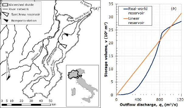
The natural flood regime of the Panaro River was observed by the Italian hydrographic service (Servizio Idrografico Italiano) in the Bomporto streamgauge station (Figure 1a) (catchment area 1036 km2, main stream length 106 km, average elevation drop 644 m, time of concentration 15 h), from 1923
to 1982, providing a 52 year long series of hourly flow discharges. This series was recorded before the Sant’Anna reservoir construction, located a few kilometers upstream of Bomporto section, so that it can be utilized to represent its hydrological input. Sant’Anna reservoir is a mainly on-line storage volume delimitated by a concrete dam, whose capacity amounts to 41.1 106 m3 between the bottom elevation
29.50 MASL and the embankment crest elevation 44.85 MASL. Its storage volume versus outflow discharge curve is illustrated in Figure 1b.
2.1 Joint distribution modelling of natural floods
To identify independent floods, the continuous time series must be separated into individual events. In this analysis, a peak-over-threshold criterion is applied to detect the partial duration series, as those periods when the observed flow discharge is greater than a threshold flow discharge qt. The independence prerequisite is matched by using a minimum interevent period IETD: successive partial durations, separated by a low flow period less than the minimum, are joined into a unique partial duration; conversely, they are considered representative of independent events.
Figure 1 Panaro River watershed (a), Sant’Anna storage-discharge curve (b).
With reference to such partial durations, the peak flow discharge qi and the flood volume v are estimated as the maximum and the integral of the total observed discharge, respectively. According to the Sklar theorem [16], their joint distribution function PQiV can be written in the terms of equation (1), where C is the underlying copula function, while PQi and PV are marginal distributions.
q,v C
P
q ,P v
PQiV i Qi i V (1)
Among the most popular families employed in flood frequency analysis, the Clayton copula is herein adopted as the most suitable solution. Its expression is reported in equation (2), where r=PQi(qi) and s=PV(v) are the uniform random variables, corresponding to the peak flow discharge and the flood volume, and is the dependence parameter. The Clayton copula belongs to the Archimedean family, suits concordant associations when is positive and features lower tail dependence properties.
1
0
1 0 0
01 1 , s , r or with , s r max s , r C (2)Owing to its mono-parametric structure, both the moment-like method and the maximum likelihood method are applicable strategies to fit the Clayton copula to data [15]. Equations (3) reports the relationship between the dependence parameter and the Kendall coefficient K, commonly employed in the copula approach to measure the association degree.
2
K (3)
The global goodness-of-fit can be assessed by using a blanket test based on the Cramer Von Mises statistics [8] defined in equation (4), where C and its empirical counterpart Cn [11] are evaluated in the pseudo-observations, derived from observed sample data according to the probability integral
transform. The sum extended to the sample size n, measures the departure of the adopted theoretical function from the empirical one. This test yields a p-value estimating the probability of the statistical error of the first type under the null hypothesis that the underlying copula is the selected one, by comparing Sn assessed for the model fitted to observed data to those assessed for a sufficiently large number of simulated samples, generated under the tested null hypothesis.
n j j j j j n n C rˆ ,sˆ C rˆ ,sˆ S 1 2 (4)Further, a proper modeling of tail dependencies plays a crucial role in the return period estimate, especially when dealing with the extreme ones. Tail dependencies can be investigated in more detail by using -plots, as suggested by [6]. These are scatter plots of the departure from independence versus the departure from bivariate median , which assume specific patterns according to the dependence structure, and can specifically focus on both upper and lower tail. A GEV distribution and a lognormal distribution are finally utilized respectively for qi and v marginals; their goodness-of-fits can be evaluated by conventional confidence boundary tests.
2.2 Bivariate return period estimation
The presence of an on-line reservoir makes the bivariate flood frequency analysis technically sound. Indeed, flood yielding the same peak outflow discharge qo can be associated with the same severity, and therefore characterized by the same return period. In order to categorize the incoming floods with respect to their severity, the reservoir routing performances must be accounted for.
To this aim, as demonstrated by [4,9], the simplified routing scheme suggested by [18] can be adopted: in this approach hydrographs are approximated to triangles both for the inflow discharge and the outflow one. In addition, the relationship between the stored volume v and the outflow discharge qo can be linearized, on condition that the storage constant k is estimated with respect to the maximum filling condition [2], as shown in Figure 1b.
This solution allows to decrease the computational burden related to the hydrograph simulation, since the peak inflow discharge qi and the flood volume v are related to the peak outflow discharge qo through an algebraic relationship. According to the derived distribution theory, the non-exceedance probability PQo is thus given by equation (5).
o
o o o
i i
i
o
Q q Pr Q |Q q Pr Q,V |VQ V kQ q P o (5)It is evident that the univariate return period derived by (5) can be attributed to all the bivariate flood events (qi,v) leading to the same value of qo. Indeed, equation (5) induces a dichotomous splitting of the bivariate population of the incoming flood events [4], which is easily delimitated in the space of probabilities [0,1]2. Therefore, P
Qo can be estimated by integrating the copula density on such regions through definite integrals.
2.3 Synthetic flood event derivation
In engineering practice, synthetic hydrographs referred to a given return period are routinely constructed from the flood reduction curve, which expresses the decreasing trend of the average flow discharge with respect to the flood duration D. According to [1], such a curve can be established in terms of reduction factor rG(D,) as shown in equation (6), where is a temporal parameter related to the characteristic watershed response times.
12 2 4 4 1 3 4 2 exp D exp D D D rG (6)As demonstrated by [13], depends on watershed geomorphologic characteristics and can be estimated with regard to the elevation drop H and the length of the main stream L, as shown in equation (7), where a and b are calibration parameters function of the geographical location and the apparent impermeability.
12
aLb H (7)
Therefore, once the peak flow discharge qi is estimated by means of the cumulative distribution function PQi, the corresponding flood volume v is derived by multiplying the reduction factor rG for the duration D and the peak flow discharge qi itself. Then, the synthetic hydrograph is completely defined by assuming a suitable shape. As suggested by [12], an effective choice is provided by a gamma function adapted to the geomorphologic reduction curve (6). The hydrograph equation (8) is thus expressed with regard to the peak flow discharge qi, a shape parameter , function of the ratio between the time to peak and the total duration, and a temporal parameter , related to the shape parameter and the flood volume v. The gamma function admits, for integer values, the analytical formulation of the reduction factor r in equation (9), where = D/ is a dimensionless duration [12]. The RFFC is finally derived through event simulations for different return periods.
q
t 1exp
t
exp
1
1
1
qt i (8) 1! 1 -1 ! 1 1 1 1 1 ! 1 1 1 1 1 1 1 1 1 1
exp i / exp / exp exp i / exp / exp exp r i i i i Γ (9)2.4 Continuous simulations
A benchmarking non-parametric version of the RFFC is also derived by a peak-over-threshold statistics of an outflow discharge series, obtained by a continuous simulation of the reservoir hydraulic behavior. All simulations were performed by using a robust procedure described in [5], and based on a Runge-Kutta numerical scheme of the fourth order.
3 Results and discussion
The minimum inter event period IETD and the threshold discharge qt needed to perform the identification of independent floods were fixed with regard to the physical properties of the catchment-reservoir system. In order to ensure that the routing processes of two subsequent floods do not interfere with each other, an IETD longer than the double of the sum of the watershed time of concentration tc and the reservoir storage constant k was used.
The threshold value qt was set in order to delete from the sample those events that are insignificant to the reservoir management. All model parameters are listed in Table 1, where is the average annual
number of events, Qi, Qi and Qi are the shape, location and scale parameters of PQi while ln(V) and
ln(V) are the location and scale parameters of PV.
A number of 5.3 floods per year is considered to be sufficiently low to satisfy the event independence prerequisite. According to this parametrization, the hypothesis that the underlying copula belongs to the Clayton family could not be rejected for a p-value of 96.5%, whilst the marginals distributions could not be rejected for usual 10% significance. The ability of the Clayton model to suit the empirical copula reveals the presence of a significant lower tail dependence, while the upper one appears to be negligible.
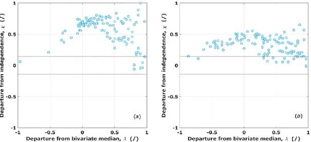
To further support this achievement, -plots obtained for the lower tail and the upper tail are reported in Figure 2, where continuous lines delimitate confidence boundaries to test tail independence for 10% significance. In this kind of test, the greater the values, the stronger the dependence is. As can be seen, in the lower tail scatter plot, (,) couples almost completely lie out of the confidence region and values rise up to one. Conversely, in the upper tail scatter plot, (,) couples are mainly included between values from 0.0 to 0.5, even if the upper tail independence hypothesis can strictly be rejected, since most of them lie out of the confidence region. Nevertheless, these -plots substantially match those that can be drawn from samples generated by a Clayton copula.
Figure 2 -plots for lower tail (a) and upper tail (b).
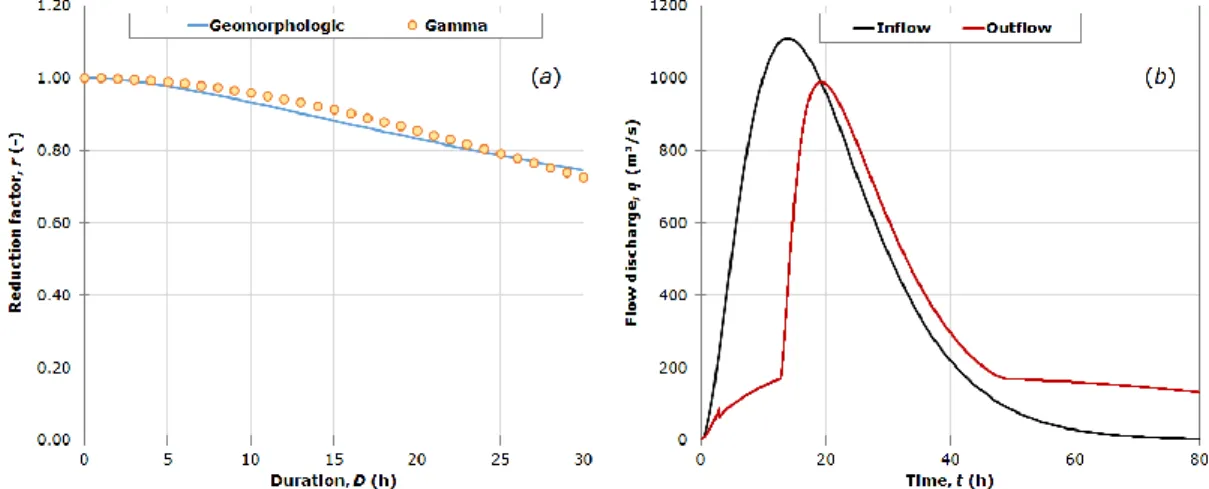
The temporal parameter assessed for equation (6) amounts to 23.4 h (a = 12.69; b = 0.64), leading to the geomorphologic reduction curve rG shown in Figure 3a. The synthetic hydrograph was defined by assuming equal to 3 and equal to 7 h, so that the reduction curve (6) is best fitted by the gamma reduction curve r (9), for durations less than 30 h. In Figure 3a the flood reduction curve r is compared to the geomorphologic reduction curve rG, and an example of individual routing simulation for a return period of 50 years is proposed in Figure 3b.
qt (m3/s) IETD (h) (a-1) tc (h) (-) k (h) Qi (-) Qi (m3/s) Qi (m3/s) ln(V) (-) ln(V) (-) 100 48 5.3 15 4.98 7.5 0.27 181.4 72.9 2.8 1.0
Figure 3 Comparison of reduction curves (a); example of a synthetic hydrograph routing (b).
RFFCs derived by using equation (5), continuous simulation statistics and synthetic hydrograph simulations are finally compared in Figure 4. A satisfactory agreement between the first and the second approach is evident, ultimately supporting the estimate method of the bivariate return periods herein proposed. Differently, the synthetic hydrograph simulation approach proves to be reliable for return periods less than 30 years; otherwise, it progressively underestimates the reservoir performances by yielding a trend close to the peak inflow discharge one.
Figure 4 RFFCs derived by continuous simulations (CS), derived distribution theory (DD) and synthetic event
simulation (SE), compared to the peak inflow discharge distribution (ID).
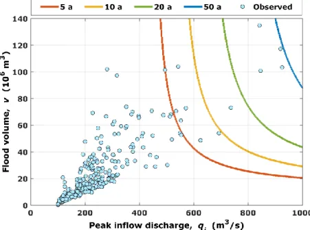
This can partially be due to the shape parameter invariance and to the assumption, implicit in the synthetic hydrograph derivation, that the flood volume has the same return period of the peak inflow discharge. Such an assumption is basically conservative. Finally, bivariate events (qi,v) featuring a mutual return period can be grouped in subsets of the population, corresponding to the iso-lines illustrated in Figure 5 for some return periods of practical interest. It is evident that, by this bivariate approach, ∞1 flood events share the same return period, as they lead to the same outflow peak
observation period is not associated with the largest flood volume but with the third one; conversely, the largest flood volume is associated with the fourth largest inflow peak discharge. The most severe event approaches the 50 year iso-line (almost the series length) and it is associated with the second largest values both for the inflow peak discharge and the flood volume. This occurrence clearly relates to the weakness of the upper tail dependence and the ability of the Clayton copula to fit the pseudo-observations.
Figure 5 Bivariate events for constant return periods.
4 Conclusions
The copula approach demonstrated to provide a very effective and straightforward strategy to construct joint distributions, yielding a satisfactory fit of the theoretical distribution function to sample data. In addition, the derived distribution theory allowed to develop a suitable estimate method for the bivariate return period of flood events. This structure-oriented approach has already successfully applied in other kinds of hydraulic applications [14,17,2,3] and appears to be the only feasible strategy to generalize the concept of return period from the univariate case to the multivariate one. It is worth underlining that a precise modeling of tail dependencies is crucial in order to derive a reliable RFFC. In this case study, the upper tail dependence demonstrated to be negligible.
However, this outcome must be regarded as site specific, so that other applications could require different copulas featuring upper tail dependence properties. The synthetic event simulation proved to be more conservative than the others for the largest return periods. This behavior suggests the need to adapt the gamma function shape when the return period increases, in order to anticipate the time to peak and to decrease the flood severity.
References
[1] B. Bacchi, A. Brath, N.T. Kottegoda, Analysis of the relationship between flood peaks and flood volumes based on crossing properties of river flow processes, Water Resour. Res. 28 (1992) 2773– 2782.
[2] M. Balistrocchi, G. Grossi, B. Bacchi, Deriving a practical analytical-probabilistic method to size flood routing reservoirs, Adv. Water Resour. 62 (2013) 37–46.
[3] M. Balistrocchi, B. Bacchi, Derivation of flood frequency curves through a bivariate rainfall distribution based on copula functions: application to an urban catchment in northern Italy’s climate, Hydrol. Res. 48 (2017) 749–762.
[4] M. Balistrocchi, S. Orlandini, R. Ranzi, B. Bacchi, Copula-based modeling of flood control reservoirs, Water Resour. Res. 53 (2017) 9883–9900.
[5] M. Fiorentini, S. Orlandini, Robust numerical solution of the reservoir routing equation, Adv. Water Resour. 59 (2013) 123–132.
[6] N. I.Fisher, P. Switzer, Chi-plots for assessing dependence, Biometrika, 72 (1985) 253–265. [7] C. Genest, A. Favre, Everything you always wanted to know about copula modelling but were afraid
to ask, J. Hydrol. Eng. 12 (2007) 347–368.
[8] C. Genest, B. Rémillard, D. Beaudoin, Goodness-of-fit tests for copulas: a review and a power study, Insur. Math. Econ. 44 (2009) 199–213.
[9] Y. Guo, B. J. Adams, An analytical probabilistic approach to sizing flood control detention facilities, Water Resour. Res. 35 (1999) 2457–2268.
[10] H. Joe, Multivariate models and dependence concepts, Chapman and Hall, London, 1997. [11] R. B. Nelsen, An introduction to copulas, second ed., Springer, New York, 2006.
[12] R. Ranzi, Structural and non-structural methods for flood hazard mitigation, Proc. of the Workshop on “Natural Environment, Sustainable Protection and Conservation: Italy-Vietnam Cooperation perspectives” Hai Phong (Viet-Nam) (2005).
[13] R. Ranzi, G. Galeati, B. Bacchi, Idrogrammi di piena di progetto dedotti dalla trasformazione afflussi-deflussi, Proc. of the XXX Convegno di Idraulica e Costruzioni Idrauliche Rome (2006). [14] A. I. Requena, L. Mediero, L. Garrote, A bivariate return period based on copulas for hydrologic
dam design: accounting for reservoir routing in risk estimation, Hydrol. Earth Syst. Sc. 17 (2013) 3023–3038.
[15] G. Salvadori, C. De Michele, N. T. Kottegoda, R. Rosso, Extremes in nature: an approach using copulas, Springer, Dordrecht, 2007.
[16] A. Sklar, Fonctions de répartition à n dimensions et leures marges, Publ. Inst. Statist. Univ. Paris 8 (1959) 229–231.
[17] E. Volpi, A. Fiori, Hydraulic structures subject to bivariate hydrological loads: Return period, design, and risk assessment, Water Resour. Res. 50 (2014) 885–897.
[18] R. L. Wycoff, U. P. Singh, Preliminary hydrologic design of small flood detention reservoirs, Water Resour. Bull. 12 (1976) 337–349.