Study of the hadronic current in the neutrino interactions of the OPERA experiment

(1)

1

UNIVERSITÀ DEGLI STUDI DI SALERNO

Facoltà di Scienze Matematiche Fisiche e Naturali

Dottorato di ricerca in Teorie, metodologie e applicazioni avanzate per la

comunicazione, l’informatica e la fisica (XI Ciclo – Nuova Serie)

Study of the hadronic current in the neutrino

interactions of the OPERA experiment

Coordinatore del Dottorato:

Prof. Giuseppe Persiano Università di Salerno

Candidata:

Dott.ssa Simona Maria Stellacci

Tutor:

Dr. Cristiano Bozza Università di Salerno

(2)

2

Acknowledgements

I would like to thank the leader of the Salerno Laboratory, Prof. G. Grella, for giving me the opportunity to work in the Emulsion Group of the Salerno University. His wide knowledge is an inspiration source and an example to do better.

Special thanks to Dr. C. Bozza for the time, the perseverance spent during the reading of this thesis. His comments and corrections were extremely useful: without them my work would have not been possible.

I wish to thank Akitaga Ariga, Tomoko Ariga and the whole group of LHEP in Bern, for making the stay in Bern a wonderful time. Special thanks to Serhan Tufanli (LHEP) for the collaboration during my time in Bern and for sharing with me the data collected in his Scan Forth analysis.

I would like to thank Dr. Umut Kose (Padova University) for the very useful help with the location bias in the Monte Carlo data.

I owe my friendly acknowledgement to Dr. Regina Rescigno for her support and encouragement during my first year of Ph.D.

Thanks to Maurizio di Marino for the technical support and support in data collection. Finally, I thank my mother for the constant help, support and the enormous endurance she proved capable of during these years.

(3)

3

Introduction

The goal of the OPERA experiment is the study of the oscillation channel νμ→ντ,

through the appearance of ντ in a pure νμ beam. The signal has the characteristic

topological signature of the decay of the charged τ lepton. Because the flight length is very short, a very high precision tracker is needed. The nuclear emulsions are the most suitable devices, thanks to their high spatial and angular resolution.

Data acquisition requires the use of automatic microscopes and the analysis of a large surface of emulsions films.

The work presented in this thesis has been carried out partly in the Salerno Scanning laboratory and partly in collaboration with the Emulsion Scanning Laboratory of LHEP-Bern, which provided data and discussion; both groups are involved in testing/validating the OPERA simulation.

The first chapter of this thesis work is an overview of neutrino physics; in the final part of the chapter some neutrino experiments are described.

The second chapter focuses on the OPERA detector. The main components of the detector are explained as well as the physical performance of the experiment.

Data-taking is the subject of the third chapter; the scanning procedure is shown, followed by the technique used to estimate the momentum of particles in the ECC. Finally, the fourth chapter presents the data analysis done by merging the data collected in the Salerno and Bern Laboratories.

(6)

6

Chapter 1 Neutrino Physics Overview

1.1 Neutrino Masses and oscillation

In the Standard Model, neutrinos are thought to be massless following the two-component theory of Landau [1], Lee and Yang [2] and Salam [3] in which the massless neutrinos are described by left-handed Weyl spinors. The Standard Model assumes that there are no right-handed neutrino fields, which are needed in order to generate Dirac Neutrino masses as in the cases of quarks.

In the last decades several neutrino experiments have collected convincing evidences of the neutrino oscillations supporting the hypothesis of neutrino masses and mixing.

1.1.1 Neutrino Masses

If one considers for simplicity only one neutrino field ψ, the Dirac mass term reads:

(1.1)

but there is no obvious reason why neutrino are more than five orders of magnitude lighter than the electron, the lightest charged particle.

In 1937 Majorana [4] developed a theory in which a massive neutral fermion can be described by a spinor ψ with only two independent components imposing the so – called Majorana condition:

(1.2)

where is charge–conjugate field, and denotes the charge– conjugation operator.

If both the left-handed and right-handed fields exist and are independent, it is possible to add to the Dirac mass term a Majorana mass that interacts with the neutrino CP-coniugate states.

(7)

7

(1.3)

where and are mass parameters and the indices R and L specify the chiral components of the neutrino field.

It is possible to add right–handed neutrinos to the SM, provided they do not appear in the standard weak interactions.

The mass term proportional to is the Majorana mass term that appears in the Lagrangian as

.

(1.4)

To find the mass states we need to diagonalise the mass matrix in eq. (1.3):

(1.5)

In the so-called “seesaw” hypothesis ([5],[6]) and , is much smaller than and is of the order of . In this case a very heavy neutrino corresponds to a very light neutrino .

1.1.2 Neutrino Mixing

For neutrinos with non–vanishing mass, the mass eigenstates with eigenvalues are not the leptonic flavour eigenstates . Mass and flavour eigenstates are connected by a unitary transformation:

(8)

8

where U is the Pontecorvo–Maki–Nakagawa–Sakata matrix. In this work, it is assumed that Majorana effects can be neglected, leaving only effective Dirac-like mass terms, thus reducing the last matrix to an identity.

The most common parameterization of the mixing matrix is

(1.7)

where and stand for the sines and cosines of the mixing angle , is the Dirac phase and ( i = 1,2,3) are the Majorana phases, set to 0 in this work.

1.2 Neutrino oscillation

The time evolution of a neutrino can be expressed as:

(1.8)

where in the ultra-relativistic limit of .

The probability to find the state after a time t, starting from the state is: (1.9)

where is the squared mass splitting, L is the distance between the source and the detector. Using the properties of U one finds:

(9)

9 (1.10) The last equation shows that the transition probability depends on the elements of the mixing matrix, on the squared mass splittings and on the parameter set by the experimental setup.

Oscillations can be observed if the mass and flavour eigenstates are different so If one considers, for simplicity, only two different flavours the mixing matrix can be written in terms of one mixing angle:

(1.11) the transition probability becomes:

(1.12)

This expression can be also cast in the shape (1.13)

The probability is given by the product of two terms bound by the interval [0, 1]. The first depends only on the mixing angle and the second on the squared mass splitting and the ratio between the source - detector distance and the neutrino energy.

The results of observations lead to estimates on , which in turn map to allowed or excluded regions in the plane by inversion of expression (1.12).

However, a full three-flavour analysis is required to consistently interpret a wide range of experimental results.

(10)

10

For the sake of completeness, it is also worth recalling that some observations would require the addition of one more sterile neutrino fields, but this debate is out of the scope of the present work, and hence it will not be mentioned further.

1.3 The effect MSW

As far, the presence of matter is not considered. The electrons the matter can affect the neutrino oscillations. The interactions with the medium can produce an effective potential that is different for different neutrino flavours.

The total Hamiltonian in matter is made by (vacuum term) plus a term, , that describes the effective potential felt by neutrinos [6]:

(1.14)

where is a flavour neutrino state ( with momentum p , is the effective potential due to the interaction with the medium. The form of is different for the charged current (CC) and neutral current (NC) scattering [7].

At energy of a few MeV, feel both the and potentials, while and feel only the potential (the energy is not enough to produce the corresponding charged lepton). In a simplified two-flavour scenario, the effective Hamiltonian is:

(1.15)

where is the density of electrons. The mixing angle becames:

(1.16)

while the squared mass splitting:

(1.17)

When A = , where = , the mixing is highest ( = , MSW resonance) as well as for low . The corresponding probability of oscillation is:

(11)

11

The MSW effect modifies the propagation of the neutrino in dense matter, possibly amplifying oscillation effects provided they already exist.

1.4 Experimental techniques to detect oscillations

Several experiments have been set up to test the neutrino oscillation hypothesis. Some use natural neutrino sources such as the Sun and cosmic rays, whereas others use artificial sources such as nuclear reactors and accelerators.

Experiments either test the appearance of neutrinos of a certain flavour or the disappearance of neutrinos of a certain flavour.

Experiments of the latter class require high statistics to measure a small effect and need accurate knowledge of the differential and integrated energy spectrum of the neutrino beam.

Appearance experiments usually deal with small statistics and do not need precise knowledge of the beam spectrum; however, they require high purity of the beam.

A complete picture is obtained by merging the data collected by several experiments using different setups. In the following, an account of the most up-to-date measurements is given, not quoting all experiments to shorten the text. Experimental techniques and results are reviewed, and a special focus is reserved to latest results with precision measurements in Section 1.5.

1.4.1 Solar Neutrinos

In the Standard Solar Model (SSM), energy production in the Sun is due to nuclear fusion of Hydrogen to Helium with electron neutrinos as by-products.

Since the 70’s the observed solar neutrino flux from all the radiochemical experiments (Homestake[8], SAGE[9], GALLEX[10], GNO[11], Kamiokande[12], SuperKamiokaNDE[13],[14]) are showed a consistent deficit (30%– 50%) compared to SSM predictions.

The most favoured explanation for this phenomenon is neutrino oscillations.

The strong confirmation that the deficit is a consequence of neutrino oscillations was provided in 2002 by the Sudbury Neutrino Observatory (SNO). Such experiment used a heavy water detector to measure the neutrino flux from the Sun. The electron neutrino could be detected via the charged current (CC) reaction , through the Cherenkov ring from electrons. The neutral current (NC) reaction, , revealed the neutrino flux through the detection of neutrons. Finally, the rate of elastic scattering (ES) events ( ) was obtained via the detection of electrons. The first reaction is possible only for the electronic neutrinos, while the

(12)

12

information about the total flux of solar neutrinos is contained in the neutral current reaction because it has a cross section independent of the flavour of the neutrino

Figure 1.1: energy spectrum of solar neutrinos (SSM)

.

The flux observed by SNO was [15]:

(1.19) (1.20) (1.21)

The results are in good agreement with the SSM and show that the solar neutrinos deficit is a consequence of the oscillation of electronic neutrino into other flavours.By combining the results of SNO and KamLAND (a detector of artificial (anti)neutrino located in Japan) with other solar neutrino experiments it is possible to estimate a more accurate value of the two oscillation parameters ([15],[16])

_(1.22)

_(1.23)

(13)

13

according to the most recent global fits.

In 2007, the Borexino experiment reported the first real- time measurement of low energy solar neutrinos. The detector, located at the Laboratori Nazionali del Gran Sasso, is a high-purity organic liquid scintillator calorimeter[18]. The aim of experiment was the measurement of the electron capture neutrinos via elastic scattering reactions by electrons at 0.862 MeV. The choice to use an organic liquid scintillator is due to the impossibility of water Cheronkov detectors to detect solar neutrinos whose energy is below 6 MeV.

Borexino founds a rate of neutrinos interactions of 47±7(stat)±12(syst) counts/(days×100 ton) [19], in agreement with the SSM provided that MSW-enhanced oscillations with large mixing occur in solar matter.

1.4.2 Atmospheric Neutrinos

Cosmic ray showers are mainly initiated by primary interactions that generate unstable particles, decaying in chain such as ,

.

The ratio of atmospheric neutrino flavours found in data is compared to expectations. The ratio (1.24) is considered in the analysis to reduce the systematic error:

(1.24)

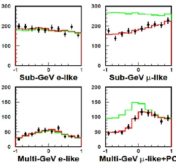
where and are respectively the numbers of events generated by muonic and electronic neutrinos. The Data and MC subscripts denote data from observations and from simulations respectively. The systematic error of this ratio does not exceed 5%. The expected value of R is 1 but the first experiments performed in the 70’s and 80’s (IMB – Kamiokande) detected about 0.6. Kamiokande performed separate analysis for both sub-GeV ( ) and multi-GeV( ) neutrinos, where

is defined to be the energy of the electron that would produce the observed amount

of Cherenkov light. The results confirmed the value of the deficit [20]: _and

[20].

The higher statistics collected by the Super KamiokaNDE experiment showed a dependence of R on the zenith angle, namely the angle between the local vertical and the reconstructed trajectory of the charged lepton[21]. Vertically downgoing (upgoing)

(14)

14

particle have cosθ = 1(-1); horizontally arriving particles have cosθ = 0. The main disappearance was observed in the neutrinos coming below the horizon that travelled for 104 km (Earth diameter) before reaching the detector. The distributions obtained by Super-KamiokaNDE suggest that the deficit increases with the distance between the production point and the interaction point in agreement with the hyphotesis of neutrino oscillations.

The plots in figure 1.2 do not show an electronic neutrino deficit; the data indicate that the favourite channel is . Furthermore the oscillation channel had been excluded by the CHOOZ experiment that studied the same region of parameters with nuclear reactor anti-neutrinos.

Figure 1.2: Event distribution in Super KamiokaNDE; the histograms show the separate distributions for muonic and

electronic neutrinos. The red line is the expected distribution without oscillation, while the green line shows the

oscillation distribution in the two flavour case . The data are depicted by points with error bars.

1.4.3 Reactor Neutrinos

The rate of inverse beta decays ( measure the flux of anti-neutrinos, which is then compared to the power output of reactors to estimate the disappearance of the electronic flavour.

The basic set up of all reactor experiments consists of identical Near and Far Detectors, or equivalently of one detector and Near-Far sources. The nuclear reactors used by the reactor experiment are pressurized water reactors (PWR). The flux of depends on the

(15)

15

power of the nuclear reactor. A modern PWR has a thermal power of 3 GWth/core and

the reactor fuel is enriched in . About 6 are produced by each reactor fission with a typical flux of core-1s-1. The four main fissile isotopes are

. Their fission rates are used as an input for the prediction of the spectrum.

The CHOOZ detector was located in an underground laboratory about 1 km from the two twin reactors of the power plant of CHOOZ in France. The CHOOZ value for was about of 300 meters per MeV, comparable to the range of atmospheric neutrinos. The main result was setting limits on the neutrino oscillation parameters related to changing electron neutrinos into other flavour.

KamLAND was surrounded by 55 PWRs; the detector, was sensitive to antineutrino oscillations in the mass mixing region suggested by the solar neutrino anomaly. The analysis of KamLAND constrained the allowed solutions for the solar neutrino puzzle to the so-called Large Mixing Angle solution.

Using multiple detectors reduces the uncertainties from reactor flux calculations, as in the case of Double CHOOZ that uses the Chooz plant. One of the two detectors sits in the same site of the previous experiment.

1.5 Precision measurements of the PMNS matrix

1.5.1

The K2K experiment

The K2K (KEK to Kamioka) experiment, which took data from 1999 until 2004, was the first long baseline disappearance experiment with artificial neutrinos. The main goal of K2K was to confirm that oscillation is the origin of the upward going atmospheric neutrino deficit observed in Super-KamiokaNDE. A pure muon neutrino beam was created by the 12 GeV proton synchroton at the High Energy Accelerator Research Organization (KEK) in Tsukuba directed towards the Super-KamiokaNDE water Cherenkov detector (Far Detector) located 250 km away. The energy spectrum and profile were measured by near detectors (ND) located 300 m from the production target. The ND consisted of two detector sets: a 1-kton water Cherenkov and a fine-grained detector system. The results found were in agreement with the neutrino oscillations parameters previously measured by Super-KamiokaNDE using atmospheric neutrinos. A total of 112 events were observed in the Super-KamiokaNDE detector while were expected without oscillations. A distorsion of the energy spectrum was observed, consistently with neutrino oscillations (Figure 1.3)

(16)

16

Figure 1.3: Energy spectrum for the observed 58 single-ring muon-like events in KEK. Points with error bars are

data. The dashed red line is the expectation without oscillation; the solid blue line shows the expectation for the best fit of oscillations parameters [22].

Figure 1.4 shows the comparison between the allowed regions of oscillations parameters found in K2K and the Super-KamiokaNDE result. The K2K result is in a good agreement with the parameters found using atmospheric neutrinos, confirming the neutrino oscillations region measured by Super-KamiokaNDE.

1

Figure 1.4: Comparison of allowed regions of oscillation parameters. Dotted, solid, dashed and dash–dotted lines

depict the 68%, 90%. 99% C.L. allowed regions of K2K and the 90% C.L. allowed region from Super-KamiokaNDE

atmospheric neutrinos, respectively [22].

The T2K experiment

The Tokai-to-Kamioka (T2K) is a long base line neutrino oscillation experiment using an off –axis design to search for the appearance of neutrinos in a beam to measure the mixing angle.

(17)

17

The T2K muon beam is produced when 30 GeV protons from the J-PARC accelerator collide with a 90 cm graphite target; these collisions produce pions that are focused by three magnetic horns and allowed to decay to muons and muon neutrinos in a 96-m long decay volume. The muons and any remaining protons and pions are stopped by a second layer of graphite. Decays of muons and kaons contaminate the beam with at the level of 1%.

T2K uses two near detectors to measure the properties of the un-oscillated beam and a far detector, the Super-KamiokaNDE detector, located 295 km away to measure the oscillated beam. The Super-K detector is 2.5° off the axis of the neutrino beams; this narrows the energy spread of the beam, with a peak tuned to the first oscillation maximum

(using the estimate from atmospheric

neutrinos,[23]).

The primary neutrino interactions mode that is of interest for T2K is the charged current quasi-elastic interaction where a charged lepton and recoil nucleons are the only particles in the final state. For such events the neutrino energy can be reconstructed as

(1.25)

where is the proton mass, is the neutron mass and the binding energy of a nucleon inside the nucleus. , and are respectively the measured muon energy, momentum and angle with respect to the incoming neutrino.

The T2K collaboration reported the observation of ten appearance candidates in a beam with data accumulated with 2.56×1020

protons on target collected by May 2012. T2K found and , in

agreement with the previous results of MINOS and Super-KamiokaNDE [24].

The MINOS experiment

MINOS searches for neutrino oscillations using the disappearance of muon neutrinos between two detectors. The Near Detector (ND) is 1 km downstream of the beam source while the Far Detector (FD) is located in the Soudan Mine, 735 km away. Both detectors are magnetized iron scintillator tracking calorimeters optimized to identify and measure the energy of muon neutrinos and antineutrinos and reject background from neutral current and interactions. Data from the ND are used to predict the neutrino energy distribution at the FD [25].

The beam is produced by directing 120 GeV/c protons from the FermiLab Main Injector onto a graphite target to produce pions and kaons that decay to produce

(18)

18

neutrinos. Two magnetic horns focus the mesons and allow controlling the energy spectrum and content of the beam. In neutrino mode the magnetic field in the horns is adjusted so that positively charged mesons are focused into the decay pipe, then decaying to neutrinos. In the antineutrino mode, negative mesons are selected, enhancing the fraction of the antineutrinos and suppressing neutrinos. In the case of the disappearance analysis, the survival probability of a muon neutrino is given by [26]:

(1.26)

The data set is based on an exposure of 3x1020 protons on target (pot); the predicted events in the Far Detector were 3564 but 2894 were observed.

The mass squared difference was found to be , and the

mixing angle at 90% C.L. [27].

MINOS has taken data in antineutrino mode and carried out an antineutrino disappearance analysis. Antineutrino oscillations are described by an equation which has the same form as equation 1.21 with parameter _and _{. The number of}

predicted events in Far Detector was 464 in the absence of oscillations, while the number of observed events was 357. The best fit of antineutrino oscillation parameters was found to be _and

_with

at 90% C.L. [27].

Muonic neutrinos may oscillate into electron neutrinos as they travel from the Near Detector to the Far Detector. The oscillation probability is given by

(1.27)

In the case of MINOS, the search for appearance is affected by large background of neutral current events that mimic charged current events. A selection algorithm is used to obtain the data sample. This selection algorithm uses a computer-intensive library event matching (LEM)1 technique to statistically separate electron neutrino events from backgrounds.

The MINOS results disfavour the hypothesis = 0 with CP – violating phase at 96% C.L.

1

The algorithm uses a MonteCarlo library of 20 million signal and 30 million neutral events to find the best 50 matches for each event and to construct three variables that are combined into a neural network to obtain a final discriminant variable.

(19)

19

Figure 1.5: Allowed ranges and best fits for as a function of CP–violating phase . The upper

panel assumes the normal neutrino mass hierarchy, and the lower panel assumes the inverted mass hierarchy [27].

1.5.2

Daya Bay

Daya Bay is a collaboration between 19 Chinese and 16 U.S. institutions; the nuclear power complex used as antineutrino source is located on the southern coast of China. It consists of six nuclear reactors grouped into three pairs. Each pair is referred to as a nuclear power plant. All six cores are functionally identical pressurized water reactors, each of 2.9 GW thermal power. Two antineutrino detectors are located in EH1, one in EH2 and three near the oscillation maximum in EH3 (the far hall, see figure 1.6, [28]).

Figure 1.6: Layout of the Daya Bay site. The dots indicate the nuclear cores of the three nuclear power plants (Daya

(20)

20

The rate in the far hall was predicted with a weighted combination of the two near hall measurements assuming no oscillation. A ratio of the measured to expect rate is defined as (1.28)

where and are the predicted and measured rates in the far hall, and are the measured background–subtracted IBD (inverse beta decays) in EH1 and EH2, respectively. The weights and are dominated by the baseline and do not depend on the integrated flux of each core; the value for the analyzed data set (collected from December 2011 through May 2012) are = 0.0444 and = 0.2991. The ratio observed at the far hall is . The value of is determined using the minimization technique; the best fit value is

[29].

T2K

To measure , T2K searches the excess of events observed in the Super–K detector that can be interpreted as oscillations. The main background sources are the beam contamination of from muon and kaon decays, and the fake - reconstructed due to interaction of . The candidate selected are required to have a single ring, and the ring must be identified as an electron-like ring. To remove the background due to photons, for each event, the mass is reconstructed and if the event is rejected. In addition, the reconstructed energy of is required to be < 1250 MeV because the probability of oscillations peaks below 1000 MeV. Then, the observed number of events is compared to the expectation based on the neutrino flux and cross-section predictions for the signal and all sources of backgrounds [30].

(21)

21

Figure 1.7: Allowed region for obtained by the T2K experiment.

The selected are used to place to constrain : _,

=0 in

the normal hierarchy hypothesis, , =0 in the inverted hierarchy hypothesis.

RENO

RENO is a Korean Collaboration that uses the six nuclear reactors of Yonggwang Nuclear Power Plant. The Near Detector is located at 294 m from the nuclear complex, while the Far Detector is at 1383 m. The ratio of found/expected events in the far detector is [31] which indicates a deficit with respect the number of events expected in the near detector assuming no oscillation. The observed spectrum of IBD prompt signals in the far detector is compared with the no-oscillation expectation based on measurements in the near detector (figure 1.5). The disagreement of the spectra provides further evidence of neutrino oscillation.

Figure 1.8: Observed spectrum of the prompt signals in the far and near detector. The backgrounds shown in the

inset are subtracted for the far spectrum. The background fraction is 5.5% for the far detector and 2.7% for the near detector; errors are only due to statistical uncertainties [31].

To determine the value of from the deficit, minimization is used and the

best fit value obtained is . This result confirms the previous measurement done by Daya Bay and is consistent with the result of T2K, MINOS and Double CHOOZ.

(22)

22

1.6 Role of the OPERA experiment and motivation of this

study

In the last years, several experiments on solar, atmospheric, reactor and accelerator neutrinos have contributed to the our understanding of neutrino mixing.

The framework is incomplete without an appearance experiment that allows observing the appearance of a from other flavours. OPERA was designed for this purpose. The main goal of the OPERA Collaboration is the observation of the appearance of in a pure beam of (CNGS), a channel that is expected to be relevant in the parameter region indicated by the atmospheric neutrino analysis.

The topological signature alone however is not able to reject all possible backgrounds from other physical processes. The signal/background ratio is increased by applying cuts, as defined in the experiment Proposal, after kinematical analysis of the final states. Such selections are used to identify the candidates (2 at the time this work was completed), and are based on Monte-Carlo simulations, whose reliability can be assessed from data from interactions of in the same CNGS beam. The present work shows the data-acquisition and comparative analysis of a “minimum-bias” sample of interactions to the standard simulation used in OPERA.

(23)

23

Chapter 2 OPERA

The OPERA (Oscillation Project with Emulsion – tRacking Apparatus) experiment was designed to observe the oscillations by detecting the appearance of in an initially pure beam of .The is revealed through the charged lepton produced in CC interactions and its decay products. Because of the short lifetime of (2.9 X 10-13 s),

a spatial resolution of ~1μm is needed whereas high density of interactions is provided by the thin lead plates interleaved with the emulsions films.

The setup of the experiment and the physical reach of OPERA are described in this chapter.

2.1 Experiment design

OPERA uses the CNGS pure muonic neutrino beam produced at CERN and sent to Gran Sasso halls where the target is placed, made with Emulsion Cloud Chambers (ECC). The ECC is a modular structure made of lead plates interleaved with nuclear emulsion plates. The so – called cell is made of a thin lead plate plus an emulsion film. The main component of the OPERA detector is the brick, a structure obtained by piling up 56 cells. By assembling a large number of bricks (about 150000 in the case of OPERA), it is possible to realise a detector optimized for the study of neutrino interactions.

This target is complemented with arrays of electronics trackers for the real-time determination of the event position and with magnetised iron spectrometers for muon identification and for the estimation of their charge and momentum.

2.1.1.a The CNGS beam

Figure 2.1 shows the main components of the beam at CERN. A 400-GeV proton beam is extracted from the SPS and is directed to the CNGS target, made of several thin graphite rods. The interaction of the beam with the rods produces secondary pions and kaons that are selected with respect to energy and charge by two lenses called horn and

reflector towards Gran Sasso. A long decay pipe allows pions and kaons to decay

mainly into and . All the residual hadrons are absorbed in a hadron stopper. Only neutrinos and muons are able to cross this 18 m-thick block of graphite and iron.

(24)

24

Muons, which are ultimately absorbed downstream by rock, are monitored by two muon detector stations. This allows the measurement of the intensity of the neutrino beam. The beam emerging from ground in the Gran Sasso laboratory has an angle of about three degrees, due to the Earth curvature.

Figure 2.1: Sketch of the CNGS beam.

The beam is optimized for the observation of interactions. The average neutrino energy is 17 GeV. The contamination is 2.1%; the contamination fractions of and smaller than 1% , while the number of prompt is negligible [33].

2.1.1.b The detector

The OPERA detector is a hybrid structure made of active and passive elements. The former are electronic devices needed to select the bricks where interactions take place and to guide the scanning, by narrowing the region of the films to be scanned. The electronic devices are also used to sample the energy of hadronic showers, to identify the muon tracks and to determine their charge and momentum.

The above-mentioned passive elements are nuclear emulsion films used as high precision tracking planes in the neutrino interaction vertex region.

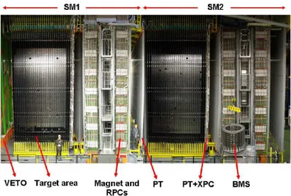
The OPERA detector, as shown in figure 2.2, is made of two identical structures called

SuperModules (SM). A SM is made of about 77000 bricks arranged in planar vertical

structures called walls, orthogonal to the beam direction. Each wall is followed by two planes of scintillator fibres, which are the building blocks of the Target Tracker (TT). The set of brick wall plus two TT planes is called module. A sequence of 29 modules followed by a muon spectrometer forms a SuperModule(SM).

The detector is also equipped with an automatic machine (the Brick Manipulator System, BMS) that allows the quick removal of bricks from the detector to study the interactions.

(25)

25

Figure 2.2: View of OPERA detector. The neutrino beam enters from the left. The target is made of walls filled with

lead/emulsion bricks interleaved with 31 planes of plastic scintillator (TT) per SuperModule. The components of the detectors are indicated by arrows. The Brick Manipulator System (BMS) is also visible [34]

The Emulsion Target

As mentioned above, the OPERA target is modular; each wall contains up to 2668 bricks for a total of 155000 bricks in the whole apparatus. The actual number of bricks is a function of time, because developed bricks are not replaced.

Emulsions films are made of two emulsion layers (44 m thick) glued on both sides of a 205 m triacetate base. The AgBr crystal yield, after development, grains with an average diameter of 0.5 m; including film-to-film alignment errors, it is possible to follow the trajectory of a minimum-ionizing particle from one plate to the next with 0.35 μm standard deviation.

The transverse dimensions of a brick are with a total thickness of about 10 X0 (7.5 cm) and a weight of 8.3 kg [35].

The brick thickness in units of radiation lengths is large enough to allow electron identification through their electromagnetic showering and momentum measurement by multiple scattering following tracks in consecutive cells. Electronic identification requires about 3 – 4 X0 and multiple scattering requires 5 X0; with 10 X0 brick

thickness for half of the events, such measurements can be done within the same brick where the neutrino interaction took place; otherwise the next brick is extracted if deemed useful [34].

The brick finding algorithm predicts the most probable brick in which the interaction occurred. The trigger is confirmed in the Changeable Sheet Doublet (CSD), a pair of emulsion sheets located outside the brick, as interface between the most downstream plate of brick and the TT.

(26)

26

Lead as neutrino beam target

Lead is used because it has a high density and a short radiation length. The former yields a high neutrino interaction rate, the latter improves the momentum determination by multiple scattering as well as the electron identification and shower energy measurements.

The residual radioactivity of the lead creates background tracks in the emulsion films and may affect the neutrino event reconstruction efficiency and purity. After dedicated tests, maximum thresholds were set on the lead radioactivity of 20 α/cm2/day and 100 β/cm2

/day .

The lead currently used produces a background of about 10 α and 50 β tracks per day per cm2 [35],[36].

The density of fake tracks created by the mismatching of unrelated low energy segments (from lead plates), can be estimated to be about 1 per mm2 after seven years, without considering fading. This value is acceptable for the energy estimation of electromagnetic showers, which is most precise when the background is low.

Target Tracker

The main purpose of Target Tracker (TT), a plastic scintillator tracking detector, is to identify the brick in which the interaction has taken place. The TT helps narrow down the region of the emulsion to be scanned to locate the interaction. The TT fibers are arranged in two planes oriented along the X and Y directions. Each plane of TT is a modular structure, made of 64 scintillator strips. Charged particles crossing the strips will create a blue scintillation light which is collected by wavelength-shifting fibers. For a minimum ionizing particle, at least five photoelectrons are detected by the photomultipliers. The detection efficiency of each plane is at 99%.

Muon Spectrometer

The spectrometer, placed downstream of each target region, allows measuring the momentum of muons and their charge. Each spectrometer consists of dipole magnet made of two magnetized iron arms producing a field of 1.52 T. Tracks are bent on the horizontal plane (parallel to ground). Each arm is made of 12 iron plates 5 cm thick. The transverse useful dimensions of the magnets are 8.75 m (horizontal), and 8 m (vertical) providing adequate geometrical acceptance for muons originating in the upstream target volume.

(27)

27

Figure 2.3: Top view of OPERA muon spectrometer. The picture shows a track trajectory along the drift tube

chambers, the XPCs and the RPCs inside the magnet. /2 is the bending angle in each dipole magnet[39].

The Inner Trackers

The Inner Trackers are Bakelite RPC interleaved with the magnetized iron plates. They allow a coarse tracking to identify muons and perform pattern recognition and track matching between the Precision Trackers and the Target Tracker. They also provide a measurement of the tail of the hadronic energy leaking from the target and the range of muons stopping in the iron[35].

The Precision Trackers

The Precision Trackers (PT) are drift tubes placed in front, in the middle and behind each arm of the dipole magnet. They determine the charge of the muons and measure the coordinates and direction of the their trajectories with a spatial resolution of 300 μm. In order to eliminate ambiguities in track reconstruction, each pair of PT is complemented with an RPC plane (the so-called XPC,[38]) equipped with pickup strips inclined by ±42.6° with respect to the ground. The RPC’s and the XPC’s also allow a more precise measurement of the momentum of muons through the bending angle. The resolution of the momentum measurement is up to 20 GeV, while the charge misidentification is below 1% for p < 25 GeV/c [39].

The Veto system

A Veto system, made of a glass resistive plate chambers, upstream of the first target area is placed. The purpose of this detector is to identify the particles of the CNGS beam produced in interactions in the rock surrounding OPERA detector. Products from these interactions can enter the detector and may induce false triggers leading to extraction and the scanning of wrong brick.

The Veto is made of two layers; each one is equipped with horizontal and vertical copper strips. The vertical array consists of 416 strips, while the horizontal of 384. In total about 1600 electronic channels collect the signal generated by the detectors.

(28)

28

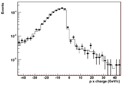
Figure 2.4: Muon momentum comparison.

Figure 2.5: Muon charge comparison (momentum × charge): the black dots with error bars are the real data, while

the solid line is the MC distribution [40].

2.2 Operation mode

The occurrence of a neutrino interaction inside the target is triggers the electronic detectors (Figure 2.6). The data collected are processed by the brick finding algorithm that predicts the most probable brick in which the interaction took place. The brick is removed from the target wall by the Brick Manipulator System and exposed to X-rays to produce 4 spots relating 4 positions between the CS doublet and the most downstream plate of the brick. Then, the CS doublet is detached from the brick and developed underground. In the CS scanning station a connection between the TT predictions and CS tracks is searched. If no connection is found, the brick is put back into the detector with a new CS doublet.

(29)

29

Figure 2.6: View of events in the OPERA electronic detector; a – like event is shown in the top of figure, while

a – like event is shown in the bottom of the figure.

If the connection is found, the brick is considered involved in the event. A further lateral set of X-rays marks fiducial positions on all the emulsion films of the brick. Then the brick is brought to surface and exposed for 12 hours to high energy cosmic rays for precise film-to-film alignment. The exposure is done in a special pit designed to provide a set of quasi-vertical hard cosmic rays (mainly muons) to be used for film-to-film alignment. The density is about 100 tracks/cm2_{. The brick is then developed and}

dispatched to one of the various scanning laboratories that locate the interaction vertex and study the event.

(30)

30

2.3 Physics Performance

The signal of the occurrence of oscillation is the charged current (CC) interaction of the tauonic neutrino inside the target ( ).

The process is identified by the detection of the τ lepton in the final state through the characteristic decay topologies of the following reactions:

17.8% (2.1) 17.7% (2.2) 64.7% (2.3)

Neutrino interactions will occur mainly inside lead plates. If the τ lepton is produced, it will decay either in the same plate (short decay) or downstream (long decay).

Figure 2.8: Schematic view of τ decay in the muonic channel. The left picture shows a short decay, while a long

decay is shown in the right picture.

In the first case, the impact parameter (IP) between the candidate τ decay daughter track is measured with respect to the primary vertex, defined by the other tracks produced in the interaction. If the value of IP exceeds 10 μm, a more accurate analysis is to be performed to completely understand the event, otherwise it is classified as an ordinary interaction. Such analysis involves the determination of the missing transverse momentum of the decay daughter with respect to the line of flight of the parent.

For long decays, the τ is detected by the kink angle between the charged decay daughter and the parent direction. As in the case of short decays, a thorough kinematical analysis follows if the kink exceeds 25 mrad (otherwise the event is classified as CC/NC). Such cuts are easily justified by comparing the distributions for and interactions. In the electronic channel (2.1), the electron is identified by analyzing its shower in the ECC.

(31)

31

For the muonic decay channel the presence of the penetrating muon track allows easy vertex identification. The presence of a kink due to large scattering on the muon track is a potential background source in interactions. Additional background components are the muonic decay of charm particles if the muon coming from primary vertex goes undetected and the muon charge assignment is wrong.

Finally, the hadronic decay channel has the largest branching ratio but is affected by high background due to charm particle decay (undetected muon from to the primary vertex) and to re-interaction of the hadrons close to the primary vertex, mimicking a decay of a short-lived particle; if the secondary interaction has a low multiplicity of products and/or some of them go undetected, the topology may fake the CC-single prong decay of the τ.

Table 2.1: Summary of the expected background for each τ decay channel.

(32)

32

Chapter 3 Data Taking Technique

The inner tracking part of the OPERA detector is made of emulsion sheets where the neutrino interactions are recorded. To read out information about topologies and kinematics of interactions, automatic systems have been developed separately in Europe (European Scanning System, ESS,[41],[42]) and in Japan (S–UTS,[43]); both have high speed, micrometric precision, high tracking efficiency and low instrumental background.

This chapter describes briefly the ESS, used in the data-taking for this work, and the techniques applied to locate and study the neutrino vertex interaction.

3.1 Images from nuclear emulsion

A few properties of emulsions have been already described. In this section, more details are presented on emulsion images, as they are the starting point for the acquisition. When a charged particle goes through the emulsion medium, it loses energy interacting mainly with the electrons inside the crystals. The average energy loss per unit length is described by the Bethe – Bloch formula:

2 (3.1) (where ).

The particle ionizes atoms along its trajectory; the excited electrons of AgBr are trapped in lattice defects creating silver atoms which act as centers of latent image.

During the development, a weak reducing agent provides electrons. The silver grains in the OPERA emulsions grow reaching a diameter of about m, becoming visible with an optical microscope.

2_{is the density, I is the average ionization potential, Z the atomic number, A the atomic weight, z the charge of the incident}

particle, v the particle velocity, the maximun energy transferred in a single interaction, the density correction, C the shell

(33)

33

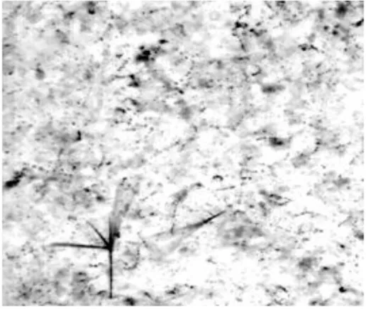
Figure 3.1: Microscope view of nuclear emulsion; the depth of field is about 5 micron.

After the development process, emulsions undergo the fixing process to remove all the remaining AgBr, leaving metallic silver grains as the image; the dissolved AgBr is removed from emulsion by washing; finally the emulsions are dried in an alcohol – glycerin bath.

The gel becomes transparent and it is possible to see the paths of charged particles, showing up as sequences of dark silver grains on a light background as depicted in figure 3.1. Most black dots in that picture are due to Compton electrons; a sizable fraction of grains is simply the “fog”, i.e. randomly developed grains, not touched by any particles produced in interactions of the neutrino beam. Dark, thick tracks are due to nuclear fragments[44].

In OPERA emulsions, made by Fuji Film, a minimum ionizing particle (m.i.p) yields 35 grains per 100 μm; a sequence of grains in an emulsion layer is usually named a

“micro-track”. The residuals of the positions of micro track grains with respect to a straight –

line fit average to 55 μm.

3.1.a Distortions

Nuclear emulsions are not rigid bodies. Apart from elastic mechanical stresses, several causes may alter their shape during processing.

Development, fixation and washing cause an increase of thickness. After drying, the final volume is smaller than the original; the decrease of volume produces an alteration on track slope parameterized with the shrinkage factor. It is defined as the ratio between

(34)

34

the thickness at the time of exposure and the thickness of the plate at the time of measurement. If one divides the slope by the shrinkage factor, the original slope is recovered.

Most commonly, distortion is a term that is related to the relative sliding of planes in the emulsion medium. Figure 3.2 sketches parabolic and linear distortion effects on microtracks:

Figure 3.2: The segment OA sketches the track without distortions; the curve OC shows the effect of parabolic

distortion on the track, while the segment OB is the track with linear distortion [44].

Whenever mutual plane sliding occurs, continuity of the deformation field implies that points close the base do not move. The parabolic distortion is due to internal stresses that vanish at the external surface. Linear distortion arises when tangential stresses are applied, e.g. by forced airflow during the drying process: the segment OB shows the effect of the linear distortion, due to the drying process that added external stresses: track slopes are modified by additive term.

3.2 Scanning Systems

Nuclear emulsions are analyzed by means of optical microscopes: by adjusting the focal plane of the objective, the whole emulsion thickness is spanned and a sequence of tomographic images of each field of view, taken at evenly spaced depths, is produced; the number of images depends on the field depth (15 is a common value for OPERA films). The main components of an automatic scanning system are:

 a motor-driven scanning stage for horizontal (XY) motion;

 a motor-driven stage mounted vertically (Z) for focusing;

 an illumination system working in transmission mode, made of a halogen lamp and a system of lenses that concentrates the light on the interesting area;

(35)

35

 a digital camera for image grabbing mounted on the vertical stage and connected to a vision processor.

In the ESS, tracking is obtained by software using commercial hardware. The S–UTS uses an algorithm coded in dedicated hardware.

ESS

The European Scanning System (ESS,[41],[40]) reaches a speed of 20 cm2/h in an emulsion layer of 44 µm thickness. By adjusting the focal plane of the objective in the whole thickness, a sequence of 15 tomographic images of each field of view, taken at equally spaced depth levels ( μ ), is obtained. The images are digitized and sent to a vision processor that applies algorithms to improve the separation of dark pixels from the background. Grains appear as clusters of dark pixels. The tracking algorithm, running on the workstation that hosts the image boards or on separate servers, recognizes microtracks as aligned sequences of such grains in the 3D volume.

S – UTS

The underlying logic of the S-UTS, used in Japan, is conceptually similar to the ESS. The main differences are the tracking algorithm described in [45], which is applied by dedicated hardware, and the continuous motion on one axis. Images are not blurred because a piezoelectric device moves the objective so as to compensate the motion of the horizontal axis, producing steady images.

3.3 Particle track reconstruction

The process of track reconstruction in OPERA is done in three steps (microtrack, base-

track and volume–track) as explained below. Microtrack

A microtrack is made of aligned grains belonging to the same layer. Several quality cuts are applied to discriminate random alignment from grain particle trajectories. With emulsion sensitivity for m.i.p. tracks of 35 grains/100 µm, the number of grains of a track in each of the two 44 µm thick emulsion layer of the film is distributed according to the Poisson law with an average of ~13 grains; microtracks not achieving at least 6 grains are discarded as random alignments.

(36)

36

Base – track reconstruction

The number of fake alignments reconstructed is reduced by connecting two microtracks belonging to the top layer and bottom layer of the same film to form a base- track. Each micro track is extrapolated to the corresponding Z level of the opposite plastic – emulsion interface and position and slope tolerances are applied to select correlated pairs.

One can define:

(3.1)

where and are, respectively, the transverse and longitudinal slope difference

between the top or bottom microtrack from the base – track slope and and are

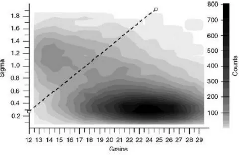
the corresponding tolerances. Two populations emerge from the sample: one with large σ value and a number of grains incompatible with the expected Poissonian law, the other one with small σ value and a number of grains well within the Poissonian expectations. The cut shown by the dashed line in figure 3.4 is applied to remove the fake base -tracks.

(37)

37

Figure 3.4: Rejection of fake base tracks based on both the slope agreement with the two micro tracks and the

number of grains: the cut shown by the dashed line is applied [42].

The resulting base track finding efficiency is about 90% over the angular range [0,700] mrad and the microtrack efficiency is about 95%

Volume – track reconstruction

A neutrino interaction at typical CNGS energies produces particles that may travel for several meters before stopping. Short–lived particles, interesting for OPERA, travel a few mm at most. Hence a region of a few cm3 is scanned around each vertex point. This requires the information from several films to be combined. The paths of charged products are reconstructed by recognizing aligned base–tracks in consecutive films. Sub-micrometric precision in film–to–film connection is obtained by exposing each brick to hard cosmic rays before disassembling (the soft component is absorbed in iron shields). After development, the pattern of cosmic ray tracks provides a reference for alignment (figure 3.5).

(38)

38

3.4 Location of the neutrino interaction vertex

The procedure to locate the neutrino interaction vertex in OPERA bricks can be sketched in the following steps:

 CS-to-brick connection  Scan–Back /Track Follow  Total Scan.

3.4.1 CS scanning

The scanning area is 16 cm2 widearound the candidate muon track for a CC event; in the case of 0-μ events (no muon in the spectrometer) the scanning area is wider and tuned according to the shape of the hadron shower, and may involve the full surface of CS doublet.

The CS candidates are required to have at least three microtrack in the 4 emulsion layers of the sheet doublet; tracks found by automatic processing are classified according to their quality, based on angular agreement and number of grains, and may be visually inspected to confirm their existence.

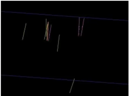
Figure 3.6: Position of the tracks found in a CS doublet; the magnitude and direction of the arrows depend on the

slopes of the tracks. A converging pattern is clearly seen.

More than one CS may be analyzed, in case the outcome of the doublet attached to the most probable brick does not confirm the presence of an interaction. If so, the first brick is put back into the detector, and the map of hits in the target trackers is checked to select another brick to be extracted, in order to locate the neutrino interaction vertex of the same event.

(39)

39

3.4.2 CS to Brick Connection

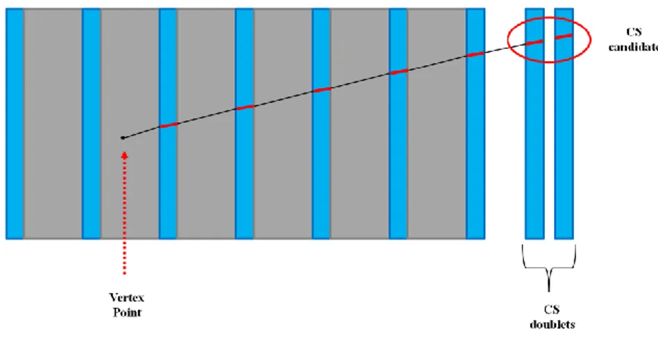
The first step to find an interaction vertex is requires locating in the brick the tracks recorded by the CS doublet. For each CS candidate, the base-tracks in the most downstream films of the brick within a position tolerance of 300 m from the extrapolated straight-line and within 40 mrad are selected (figure 3.7).

Figure 3.7: The positions of CS candidates are projected on brick plates; the five most upstream plates are scanned

for CS candidates. The tracks that pass the cuts in position and slopes are followed in the brick downstream to arrive at the interaction vertex.

(40)

40

3.4.3 Scan-Back/Track Follow

The CS candidates connected are followed back to locate the point where they disappear (which is indeed the place where they are produced). Two techniques are used, namely “Scan-Back” (SB) and “Track Follow” (TF).

Scan-Back (see figure 3.9) is based on scanning single microscope views centered on the track position in each film. After finding the track in each film, the position and slopes are updated for the next upstream film. The coordinates are projected to the next upstream plate and the track is searched for by the automatic system. The tolerance required is as large as 50 m on position (because no fine alignment is used at this stage) and 20 mrad on slope. The process is repeated until track disappearance. A track may be missed because of the non-vanishing inefficiency of tracking and/or defective images (because of dust or scratches), or just due to low ionization. Depending on the data quality, a number of 3 – 5 consecutive films without a suitable track candidate are required to define a stopping point.

To reduce the workload for visual inspection and fake interaction points, the Track Follow (TF) procedure is progressively replacing SB. In TF, CS candidates are followed down plate by plate in the entire brick. One does not attempt to identify the right track at each film while scanning; a “tower” of 3×3 mm2

, centered on the position predicted by the CS candidate and skewed with the track slope is scanned through the whole brick, and offline analysis is used to identify the stopping point.

Figure 3.9: Scan Back procedure: CS candidates are searched in the brick. Emulsion films are in blue, while the lead

plates are grey. The base-tracks found in the plate are shown in red.

The advantage of TF (figure 3.10) is at least twofold: first, it allows individuating multi-prong vertices already in this stage; furthermore, data can be merged with those taken in the Volume Scan.

(41)

41

Figure 3.10: Track Follow procedure: the track is followed back in the brick. The scanning area is 3 mm x 3mm and

skewed with the track slope.

If the SB/TF track exits the brick, it has to be followed into the brick it is pointing to. Another brick is extracted from the detector and developed.

3.4.3 Total Scan

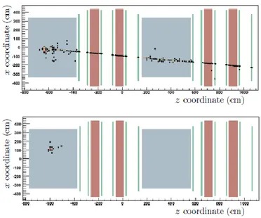
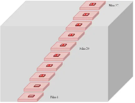
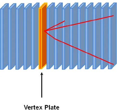
The confirmed stopping point is used to launch a scanning of a large volume; in the so– called Total Scan (TS), an area of 1×1 cm2 is scanned (figure 3.11) on 5 films upstream of the track disappearance film and 9 films downstream. Tracks are measured within a slope acceptance of 0.5. Geometry software performs alignment and topology reconstruction software analyzes the scanning data and yields tracks and decay/interaction vertices.

(42)

42

Figure 3.11: Schematic view of volume scan. The yellow plate is the vertex plate; in this stage an area of 1 cm2

around the stopping point is scanned. The picture shows a sketch of primary interaction.

3.5 Event study: the decay search

The decay search procedure allows discriminating interesting topologies like charm or candidates from the majority of νμ or νμ interactions.

Decays of particles produced at the primary vertex are classified as “short” if they decay in the same lead plate of the neutrino interaction, “long” otherwise.

The decay search procedure has specific branches for the various possible topologies and geometries.

Hard tracks (P > 1 GeV) attached to the primary vertex are checked for “in–track” decays, i.e. small kinks (<30 mrad) that went undetected through the topological reconstruction because they fall below the tolerance for film-to-film connection. This allows detecting long decays with small transverse deflection. The slopes of the first five segments are checked to make sure that the kink is statistically outstanding from the background due to background of scattering and measurement errors.

The “extra-track search” looks for possible daughter tracks produced in decays and not connected to the vertex (either because the decay is short or because the decay parent track has not been recognized). The possible decay candidates are particles with a momentum >1GeV that disappear close to primary vertex, and an Impact Parameter (IP) exceeding 10 . The geometrical information from emulsion is matched to the CS doublet and the electronic detectors to make sure that the track is related to the event.

(43)

43

Event that show decay kinks are investigated to collect further data to perform kinematical analysis.

3.6 Event study: characterization of the interaction products

Track followed from the CS back to the primary neutrino interaction can be immediately used for kinematical analysis; in most cases, however, and they are only partially contained in the volume scanned around. In order to estimate their kinematical parameters, further data-taking is required.

Tracks found at the interaction vertex and that were not followed from the CS doublet to the interaction point require additional data–taking. This procedure is called Scan–Forth (SF) and is similar to SB; or it may be replaced with a TF–like data taking, downstream from the vertex plate.

The steps are the same as in the case of primary vertex location: if a track stops in the brick, this may be due to an interaction (typically hadronic). In such case, another volume is scanned around the confirmed stopping point, with 1 cm2 area on 5 plates upstream and 5 downstream the interaction point. Automatic reconstruction is then used to detect the topology of secondary interaction.

For muons, the spectrometer provides the best determination of the momentum; hadron momenta are instead estimated from track measurements in the ECC with the method of Multiple Coulomb Scattering (see below).

Figure 3.12 Schematic view of SF data–taking: tracks are followed from the primary vertex; the white track shows a

secondary interaction, so a large volume scanning is performed.

SF and TF can distinguish between hadrons and electrons (which soon show electromagnetic showers from bresstrahlung photons); muons are identified through angular and momentum matching with muon tracks seen in the electronic detectors.

(44)

44

Once momentum estimation and particle identification are complete for all tracks produced at the primary vertex, all the needed data are available for the kinematical study of the event. It is worth pointing out that the electromagnetic component is excluded from this analysis because photons may convert within the brick/wall supports, or in any case out of the first brick; complete collection of the electromagnetic component would require a scanning effort beyond practical reach if applied for all events

Example of the detection of a secondary interaction: event 9299027091

Event 9299027091 is a good example of the thorough study of an event in OPERA ECC. Figure 3.13 shows the electronic display of the event.

The brick where the interaction occurred has number 76351. The CS candidates connected to the brick were three; a track with slopes close to the muon measured in the TT was one of them3.

The TF was launched around all CS-connected tracks; the volume scan was launched around the stopping point of the muon-like followed track. The decay procedure was applied at the stopping point, found on plate 21. The tracks attached to the primary vertex were six, and two pairs were detected. The tracks at the primary vertex are followed in SF, except the electron pairs. The momenta were computed by the algorithm described in [46]. The momentum of the muon in emulsion was

GeV, while the momenta of other tracks are shown in table. A secondary interaction was found following one track; an additional large-area scanning was launched to confirm the presence of secondary tracks seen in emulsion. The tracks attached at the secondary vertex are five. The tracks of the secondary vertex were followed in Scan-Forth mode until plate 57, where they leave the brick. Figure 3.14 shows the reconstructed event.

(45)

45