Innovative techniques for Structural Health Monitoring: a

D

IPARTIMENTO DI

I

NGEGNERIA

M

ECCANICA

Dottorato di Ricerca in Ingegneria Meccanica

IX Ciclo N.S. (2007-2010)

“Innovative techniques for Structural Health Monitoring: a

theoretical and experimental study”

Ing. Rossella Valiante

Tutor:

Coordinatore:

Prof. Domenico Guida

Co-Tutor:

Prof. Fernando Fraternali

Ing. Generoso Iannuzzo (Alenia)

Prof. Vincenzo Sergi

The present work, carried out at Alenia Aeronautica,

The present work, carried out at Alenia Aeronautica,

The present work, carried out at Alenia Aeronautica,

The present work, carried out at Alenia Aeronautica,

contains sensitive information and data covered b

contains sensitive information and data covered b

contains sensitive information and data covered b

contains sensitive information and data covered by the

y the

y the

y the

Intellect

Intellect

Intellect

Intellectually Property Rights. Therefore,

ually Property Rights. Therefore,

ually Property Rights. Therefore,

ually Property Rights. Therefore, the use of

the use of

the use of

the use of

such information and data is allowed only under

such information and data is allowed only under

such information and data is allowed only under

such information and data is allowed only under

permission of Alenia Aeronautica.

permission of Alenia Aeronautica.

permission of Alenia Aeronautica.

permission of Alenia Aeronautica.

RINGRAZIAMENTI

E’ per me doveroso, oltre che sentito, ringraziare l’ing. Iannuzzo, il quale, oltre ad avermi supportato come tutor nella stesura del presente lavoro, mi ha, innanzitutto, concesso la preziosa possibilità di affrontare quest’avventura.

Vorrei, inoltre, dire il mio forte grazie al prof. Guida che, non pago di avermi sopportato durante la tesi di laurea, mi ha invogliato a tentare questo arduo percorso, ancora una volta sotto la sua guida.

Un ringraziamento particolare lo dedico al prof. Fraternali, il quale mi ha fornito lo sprone necessario a seguitare col lavoro di dottorato, oltre ad avermi guidata attentamente nella stesura dello stesso.

Non posso dimenticare il prof. Ruzzene, che mi ha introdotto nel mondo delle onde di Lamb, né la sua collaboratrice, Nicole Apetre, la quale tanti preziosi consigli sulla modellazione numerica delle stesse mi ha dispensato.

Tengo particolarmente a ringraziare il Prof. D’Agostino che, col garbo che lo contraddistingue, ha seguito, seppur da lontano, quest’altro mio percorso di studi, dandomi sempre l’impagabile sensazione di sentirmi a casa ogniqualvolta mettessi piede a Fisciano.

Ringrazio il nostro Coordinatore, Prof. Vincenzo Sergi, per la gestione ineccepibile del corso di dottorato, accompagnata sempre da atteggiamento disponibile e cortese.

Dico grazie infinite a Pierpaolo D’Agostino, che mi ha più volte salvato dal panico ‘da dottorato’, oltre che aiutato fattivamente in questi tre anni sempre col sorriso sulle labbra. Grazie, Pierpaolo!

Non posso dimenticare Luca, Rosario, e tutte le persone coinvolte nel coordinamento del corso, né i miei colleghi d’avventura, Roberta, Marzia, Gino, Renzo, sempre disponibili e gentili.

Vorrei, inoltre, ringraziare il collega Michele Rotondano, per il suo fondamentale contributo informatico.

Un mega grazie va alla mia amica, nonché collega, Maria Pagano, per la preziosa collaborazione ed il supporto morale! Merci, Mary!

Particolarmente doveroso ed al contempo piacevole per me ringraziare Damiano Laurenza, il quale mi ha fornito aiuto concreto, oltre ad avermi spronata ad ogni ostacolo incontrato sulla via. Grazie!

Tengo a dire grazie alle mie super amiche Ylenia e Stefania, per l’incoraggiamento continuo ricevuto, sempre e comunque. Grazie, tesorucce!

Ringrazio l’Amico cui devo moltissimo, don Dolindo; un ringraziamento particolare lo dedico a don Peppino, imprescindibile presenza di questi anni.

Un grazie speciale lo dedico alla persona più che speciale che mi ha letteralmente sopportato, oltreché sopportato in questo periodo, con una presenza delicata e costante. Grazie di cuore.

Vorrei, infine, disporre del vocabolario di Dante per dire grazie alle persone della mia famiglia, papà, mamma e Pina, le quali mi hanno dato, ciascuna a proprio distintivo ed unico modo, la forza di raggiungere il traguardo. Vi amo.

A PAPÀ, MAMMA E PINA,

RISPETTIVAMENTE IL MIO CUORE,

LA MIA ANIMA E

CONTENTS

Abstract of dissertation ... 7

1.

Introduction...10

1.1. General SHM Paradigm ...12

1.2. Definition of Damage in CFRP Composite Components ...13

1.3. Global versus Local SHM Approaches...15

1.4. Vibration-Based Vs Guided Waves-Based Techniques: Our Choice ...16

1.5. Vibration-Based Damage Measures ...18

1.5.1.

Frequency changes... 18

1.5.2.

Mode shape changes ... 20

1.5.3.

Mode shape curvature changes ... 21

1.6. Guided Waves-Based Damage Measures...23

1.7. Theory of waves in elastic media ...24

1.7.1.

Waves in taut string ... 24

1.7.2.

String on an elastic base – Dispersion ... 28

1.7.1.

Group Velocity... 34

1.7.1.

Wave in plates - Lamb waves ... 37

2.

Innovative

SHM Techniques based on SLDV measures ...43

2.1. Damage measure based on Energy functional distribution ...44

2.2. Interpolation of the measured response and synthesis of the undamaged baseline ...46

2.3. Strain Energy Distributuion...48

2.4. Filtering of signals in domain wavenumber / frequency...49

3.

Experimental Analysis ...53

3.1. Description of the measure set up ...56

3.2. Acquisition parameters ...56

3.3. Results ...60

3.3.1.

Skin External Side... 62

3.3.2.

Skin Internal Side ‘1’ ... 63

3.3.3.

Web Side ‘1’ ... 66

3.3.4.

Skin Internal Side ‘2’ ... 68

3.3.5.

Web Side ‘2’ ... 70

3.5. First Conclusions ...74

3.6. Elaboration of the SLDV data previoulsy observed ...76

3.6.1.

Skin External Side... 76

3.6.2.

Skin Internal Side ‘1’ ... 79

3.6.3.

Skin Internal Side ‘2’ ... 82

3.6.4.

Web Sides ‘1’ e ‘2’ ... 85

3.7. Comparative Analysis of the Signals recorded on the opposite sides of the web ...91

3.8. Analysis of further Polytec data ...96

3.8.1.

Test and Item description... 97

3.9. Results recorded by Polytec with a 3D vibrometer over a plate with defects...99

3.10. Polytec Data Post-processing by means of propagation maps of the reflected waves and damage maps ...103

3.11. Conclusions ...107

4.

Finite Element Modeling of wave propagation in anisotropic

strengthened plates...109

4.1. Overview of Explicit Dynamic Analysis for MDNASTRAN SOL700...110

4.2. Geometry of model ...114

4.3. Modeling of the examined plate by shell elements...116

4.4. Loads and constraints...120

4.5. Material properties and lay-up ...123

4.6. Wave propagation in F.E. model with shell elements...124

4.7. Modeling of the examined plate by solid elements ...126

4.8. Material properties and lay-up ...127

4.9. Wave propagation in F.E. model with solid elements ...127

5.

Conclusions and future work ...131

LIST OF FIGURES AND TABLES

Fig. 1.1 - Scheme of SHM based damage identification process. ... 12

Fig. 1.2 - Guided waves propagating within a confined geometry. ... 23

Fig. 1.3 - Differential element of taut string. ... 25

Fig. 1.4 - Deflections of an infinite long string at successive times ... 27

Fig. 1.5 - Undistorted propagation of wave envelope... 28

Fig. 1.6 - Differential element of a string on an elastic base ... 29

Fig. 1.7 - Distorted propagation of a wave envelope... 31

Fig. 1.8 - Frequency spectrum for a string on an elastic foundation ... 33

Fig. 1.9 - Two-dimensional representation of the frequency spectrum

showing relation between chord slope and phase velocity ... 33

Fig. 1.10 - Dispersion curve for a string on an elastic foundation... 34

Fig. 1.11 - Group velocity example ... 36

Fig. 1.12 - Group velocity variation with phase velocity ... 37

Fig. 1.13 - Directions of particle motion for the case of harmonic waves in

infinite media ... 39

Fig. 1.14 - Symmetric and anti-symmetric Lamb wave modes ... 41

Fig. 1.15 - Phase velocity dispersion curves for an aluminum plate ... 42

Fig. 1.16 - SH wave mode propagation ... 42

Fig. 2.1 - Flowchart of SHM based damage identification process... 45

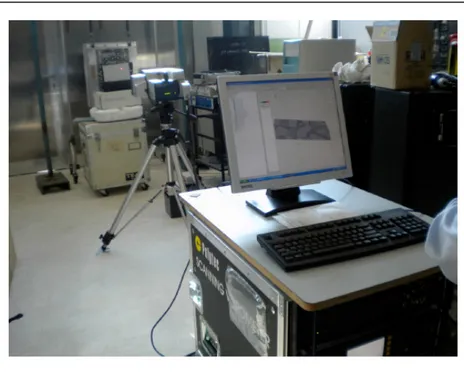
Fig. 3.1 - Laser Vibrometer used for the tests and for the data acquiring

system ... 54

Fig. 3.2 - Voltage amplifier and signal generator employed for piezoelectric

excitation... 54

Fig. 3.3 - Component under test... 55

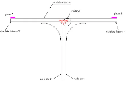
Fig. 3.4 - Section with a horizontal piano of the component under test, with

indication of the position of the actuators used for the tests, of the

nomenclature of the different subcomponents analyzed and of the area

subject to potential wrinkling... 55

Fig. 3.5 - Schematical description of the measurement setup utilized... 59

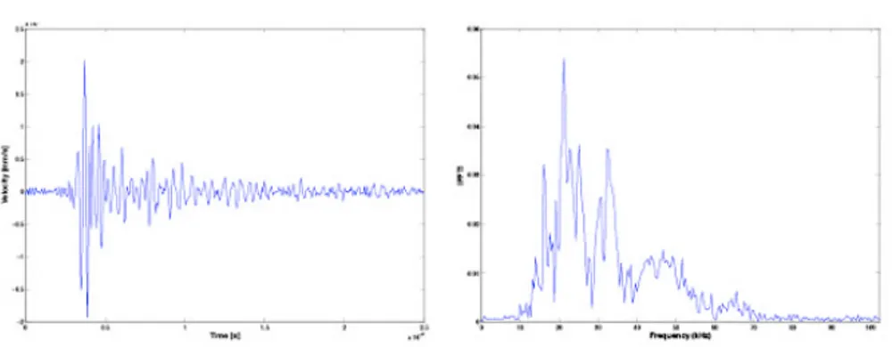
Fig. 3.6 - Impulse generated in entrance (left) and corresponding Fourier

Transform (right) ... 59

Fig. 3.7 - Signal recorded corresponding to a measure point of the laser

vibrometer (left) and corresponding Fourier Transform (right). ... 60

Fig. 3.8 - Pattern of the lamb waves excited in the component under test .. 61

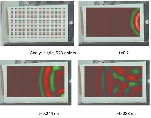
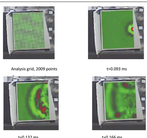
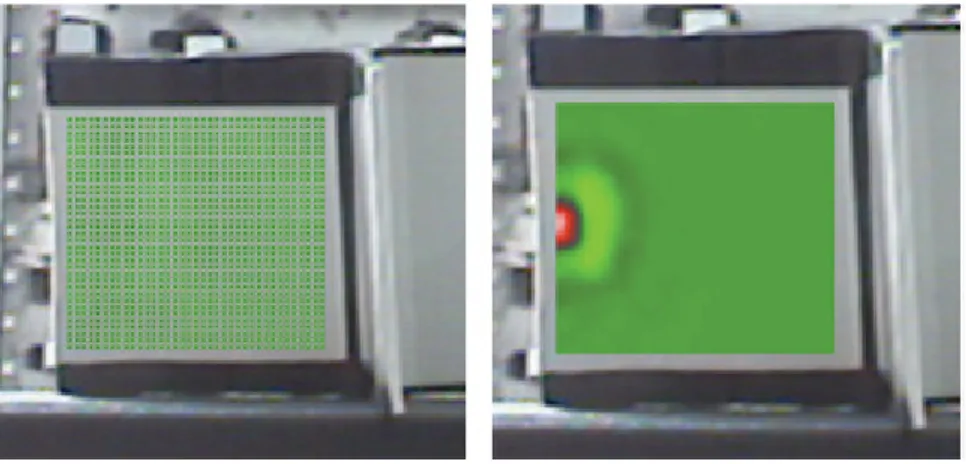
Fig. 3.10 - Sampling grid and snapshots of the wavefront at various instants

on the skin external side... 62

Fig. 3.11 - RMS map on the skin external side... 63

Fig. 3.12 - Sampling grid and snapshots of the wavefront at various instants

on the skin internal side 1 ... 64

Fig. 3.13 - RMS map on the skin internal side ... 65

Fig. 3.14- Detail of the area with reducing thickness partially responsible for

the energy concentration. ... 65

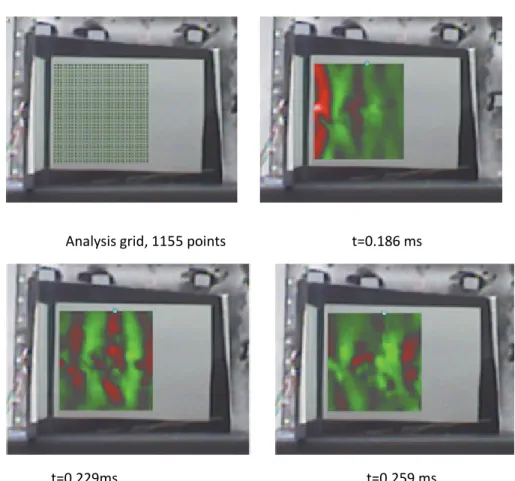
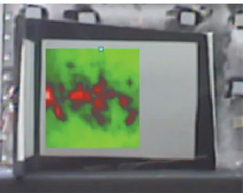
Fig. 3.15 - Sampling grid and snapshots of the wavefront at various instants

on the webside 1... 66

Fig. 3.16 - RMS map on the web side 1... 67

Fig. 3.17 - Detail of the area potentially concerned by high porosity ... 68

Fig. 3.18 - Sampling grid and snapshots of the wavefront at different

instants on the skin internal side 2 ... 69

Fig. 3.19 - RMS map on the skin internal side 2 ... 70

Fig. 3.20 - Sampling grid and snapshots of the wavefront at different

instants on the web side 2 ... 71

Fig. 3.21 - Map of the mean square recorded during the time of the

vibration velocities measured on web side 2 ... 72

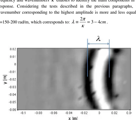
Fig. 3.22 - Wavelenght highlighted in a snapshot of the wavefront on the

skin... 73

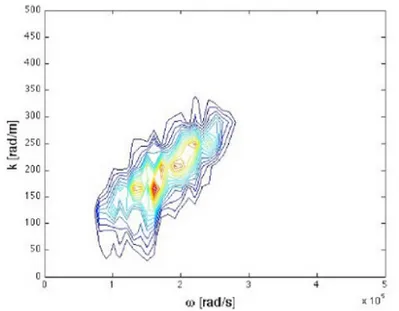
Fig. 3.23 - Representation of the response measured in the domain

wavenumber/frequency... 74

Fig. 3.24 - Photograms of the whole wave field (incident waves plus

reflected waves) on the external side of the skin at given time intervals. ... 77

Fig. 3.25 - Photograms of the field of reflected waves on the external side of

the skin at given time intervals. ... 78

Fig. 3.26 - RMS of the field of reflected waves on the external side of the

skin... 79

Fig. 3.27 - Photograms of the whole wave field (incident waves plus

reflected waves) on the internal side '1' of the skin at given time intervals. 80

Fig. 3.28 - Photograms of the field of reflected waves on the internal side '1'

of the skin at given time intervals. ... 81

Fig. 3.29 - RMS of the field of reflected waves on the internal side '1' of the

skin... 82

Fig. 3.30 - Photograms of the whole wave field (incident waves plus

reflected waves) on the internal side '2' of the skin at given time intervals. 83

Fig. 3.31 - Photograms of the field of reflected waves on the internal side '2'

of the skin at given time intervals. ... 84

Fig. 3.32 - : RMS of the field of reflected waves on the internal side '2' of

the skin. ... 85

Fig. 3.33 - Photograms of the whole wave field (incident waves plus

reflected waves) on the side '1' of the web at given time intervals ... 86

Fig. 3.34 - Photograms of the field of reflected waves on the side '1' of the

web at given time intervals ... 87

Fig. 3.35 - RMS of the field of waves reflected on side '1' of the web... 88

Fig. 3.36 - : Photograms of the whole wave field (incident waves plus

reflected waves) on the side '2' of the web at given time intervals... 89

Fig. 3.37 - Photograms of the field of waves reflected on side '2' of the web

at given time intervals ... 90

Fig. 3.38 - RMS of the field of waves reflected on side '2' of the web... 91

Fig. 3.39 - Analysis grid used on the side 1 of the web (WEB1) overlapped

to the RMS map of the whole travelling wave on the same side. ... 92

Fig. 3.40 - Analysis grid used on the side 2 of the web (WEB2) overlapped

to the RMS map of the whole wave travelling on the same side. ... 93

Fig. 3.41 - Diagrams velocity-time in correspondence to symmetrical points

of sides 1 and 2 of the web, properly vertically offset... 94

Fig. 3.42 - Fourier transform (FFT) of the signals shown in pic. 3.40,

properly vertically offset... 95

Fig. 3.43- Total energy versus positions graphs (WEB 1 and 2)... 96

Fig. 3.44 - Polytec test setup... 97

Fig. 3.45 - Impact locations. ... 98

Fig. 3.46 - Measurements of the delaminations... 99

Fig. 3.47 - Excitation signal in time representation. ... 100

Fig. 3.48 - Zoomed view of the excitation signal in time representation .. 100

Fig. 3.49 - Excitation signal in spectral representation... 100

Fig. 3.50 - Response of a stiffened plate at a 270 kHz excitation applied

through piezoelectric actuators on the bottom: vibrations in Z (a) directions

and vibrations in Y (b) directions. The locations of real damages have been

highlighted with black circle, while areas of incorrect damage indications

have been highlighted with red ones... 102

Fig. 3.51 - Photograms of the whole wave field (incident wave plus

reflected wave) at given time intervals ... 105

Fig. 3.52 - Photograms of the whole wave field (incident wave plus

reflected wave) at given time intervals ... 106

Fig. 3.53 - Damage index map with detailed indication of damaged zones

(yellow ovals)... 107

Fig. 4.2 - Explicit scheme diagram ... 112

Fig. 4.3 - Skin geometry ... 114

Fig. 4.4 - Item profile including skin and stringers... 115

Fig. 4.5 - Panel geometry (view from above) ... 115

Fig. 4.6 - Panel geometry (frontal view)... 115

Fig. 4.7 - Panel geometry (lateral view) ... 116

Fig. 4.8 - Cut-off of the total panel meshed ... 118

Fig. 4.9 - Enhancement of meshing. ... 118

Fig. 4.10 - Pure modes by excitation of the plate on both sides ... 120

Fig. 4.11 - Input excitation signal in time and frequency domain, 5.5 cycles

at 270 kHz ... 121

Fig. 4.12 - Loads and constrains on the model ... 122

Fig. 4.13 - Details of previous image... 122

Fig. 4.14 - Property set name scalar plot ... 123

Fig. 4.15 - Field output of the out of plane velocity

V

₁

for stiffened plate

with delamination, modeled with shell elements ... 125

Fig. 4.16 - Cut-off of the total panel meshed with hex8 elements... 126

Fig. 4.17 - Enhancement of meshing. ... 126

Fig. 4.18 - Field output of the out of plane velocity

V

₃

for stiffened plate

with delamination, modeled with solid elements... 129

Fig. 4.19 - Plot of the velocity recorded from the laser vibrometry at

different time instants. ... 130

ABSTRACT OF DISSERTATION

Aerospace industry is characterized by continuously growing safety cost requirements. This fact leads to the exponential increase in the use of composite materials. With such feature as high strength-to-weight and stiffness to weight ratios, these materials allow the manufacturing of lighter and more efficient structure, with respect to aluminum alloys, in order to increase the payload and to reduce the fuel consumption. However, composite structures are very vulnerable to structural damage, in particular to the delamination that can be introduced during manufacturing or service. The occurrence of delamination could potentially lead to a catastrophic failure of the whole structure, if it accumulates above a critical level. Cost saving must never be considered without safety. For this reason, in the last years researchers have been developing ever more sophisticated damage monitoring systems, which are able to evaluate the health of a structure in real-time. This branch of research is known as Structural Health monitoring (SHM).

This study investigates the use of Lamb waves and laser vibrometry for the identification and localization of damage/defects occurring within critical components of aircraft structure. In the present study, a SHM strategy based on dynamic structural analysis performed over a wide frequency range is presented. The frequency band of investigation spans from the lowest mode of the structure up to the low ultrasonic range, and so, potentially, it allows the detection of various sizes of defects. The tests are performed using a single actuator/sensor pair: piezoelectric discs are employed as actuators, while a Scanning Laser Doppler Vibrometer is used as a sensing device. The piezoceramic discs are inexpensive and easy to operate and the Scanning Laser Doppler Vibrometer measures the velocity of the structure at points on a user-defined grid, thus providing an unprecedented amount of information.

The aim is to obtain a comprehensive structural monitoring methodology able to overcome drawbacks and exploit advantages of various techniques. In the low-to-medium frequency range, modal parameters are normally less sensitive to localized defects, but generally provide indications regarding global changes as a result of damage. Such changes localize defects and potentially estimate their severity. In addition to modal monitoring, the Scanning Laser Doppler Vibrometer is used as an ultrasonic sensor. The two techniques are applied sequentially: vibration-based monitoring first provides indication of potential areas of damage, on which the scanning laser Doppler vibrometer then focuses to perform ultrasonic testing and to obtain detailed damage information. The technique is demonstrated experimentally on plate-like stringerized structures affected by artificial delaminations or by wrinkling caused by manufacturing process and, subsequentially, on numerical models of the previous tested components. The approach followed in this thesis is divided into five chapters.

The first one presents a description of the SHM, along with the state of the art on this technique. Moreover a brief introduction to the theory of waves in solid materials is provided. Then, in the second chapter the description of the two innovative SHM techniques (i.e. the signal filtering technique in wavenumber-frequency domain and the comprehensive damage index), developed by Ruzzene and on which this work relies on, is extensively described. The third chapter is centered on the innovative experimental analysis carried out at Alenia Aeronautica laboratories in Pomigliano. An explanation of the experimental setup is provided along with the obtained results. Then, the post-processing techniques, explained in the previous chapter, are applied and the obtained results are reported. In the fourth chapter the two adopted FE modeling techniques (with CQUAD4 elements and with HEX8 elements) are extensively described, focusing on the possibility of correctly modeling the wave propagation in composite strengthened plates through the use of the finite element method (there are no published works in this field, regarding strengthened panels). This is no trivial task because of the complex nature of wave propagation in plates, especially for the composite materials case. Then, the confrontation between experimental data and the numerical approach is reported. In the fifth chapter conclusions and future work are reported.

The most significant technological innovations achieved through this work are:

• The option key to excite the surface of a complex structure (in this case, the skin of a composite stringerized panel) and to derive the velocity profile on a surface which is orthogonal to the excited one (in our case the web of the stringer) has been checked. Obviously, in such a way, it is also automatically validated the opposite approach. This is crucial, since it would allow technicians to install fixed piezo elements on the stringers, to excite them (when the plane is in the hangar) and to read velocities of points over the entire surface of the skin, without disassembly. A configuration of great practical utility may be obtained permanently placing some actuators on the two opposite sides of the web and measuring the response on the external side of the skin, easily accessible.

• Up to now, only cases of standard solicitation (i.e. cases in which the velocities were acquired on the same surfaces excited) have been analyzed in literature.

• The Damage Index has been also applied to greatly complex geometries. Up to now, in literature only articles concerning tests on simple flat panels can be found.

• The FEM simulation has been carried out on stiffened panels. In literature, only works regarding simulations carried out on simple structural elements like flat panels without any stiffener can be found.

1.

INTRODUCTION

All civil, mechanical and aerospace structures are subject to damage as a result of fatigue, overloading conditions, material degradation through environmental effects and unanticipated discrete events such as impacts or seismic events. Damage compromises the ability of the structure to perform its primary functions. Therefore, to ensure performance standards, extend the operational lifespan and maintain life-safety, many structural systems undergo routine inspections and maintenance. Common non-destructive evaluation (NDE) methods for evaluating the integrity of a structural component include the use of Eddy currents, acoustic emission, ultrasonic inspection, radiography, thermography or just basic visual inspections [1]. Depending upon the structural system, the cost associated with systematic time-based NDE inspection and maintenance can be substantial relative to the total life-cycle costs of the system. For commercial and military aircraft, it is estimated that 27% of the average life cycle costs are related to inspection and repair [2]. In addition, there is a corresponding opportunity cost associated with the loss in operational availability during maintenance. Within the aircraft industry in particular, maintenance procedures are dependent upon the design methodology adopted for the vehicle components.

The two dominant design methodologies are safe-life and damage tolerant [1]. For safe-life design, the operational lifespan of structural components is estimated through a statistical analysis. Inspection is not necessary for this methodology, since the components are simply replaced prior to its specified design life. As a result, safe-life design is the least economical. Currently, many aircrafts are designed according to damage tolerant methodology. In this approach, models are used to predict the emergence of damage in various components under specified loading conditions. Based upon these models, NDE (Non Destructive Evaluation) inspection and preventive maintenance is performed at frequent time intervals to identify incipient damage and to prevent critical damage growth. An effort is currently being made to implement a newer condition based design methodology. In this case, maintenance is only performed when the system has undergone damage beyond a tolerable level.

Ideally, routinely scheduled inspection would be replaced by the integration of a built-in structural health monitoring (SHM) system that can perform continuous on-line diagnostics as well as prognostics. The objective for the diagnostics is to perform damage identification while the prognostics allows for an estimation of the remaining useful life of the system. Condition based maintenance, based upon a SHM philosophy, is the most economical option. Ideally, an SHM system will increase the operational availability, extend the lifespan of an aircraft, enhance life-safety and dramatically reduce life-cycle costs. It is estimated that a savings of 40% on inspection time and 20% on inspection/maintenance costs could result from the implementation of a properly designed SHM system [1].

The function of an SHM system is to collect periodically sampled dynamic response measurements of the structure using an integrated network of strategically placed transducers [3]. From these measurements, extracted damage sensitive features are then used to solve a forward or inverse problem with system models or applied in statistical pattern recognition algorithms in order to evaluate the structural condition of the system.

One of the primary objectives of an SHM system is damage identification. Damage identification can be organized into a hierarchical pattern as follows [4]:

Level 1 (Damage Detection): Recognition that damage exists within the structure

Level 2 (Damage Localization): identification of the geometric position of damage

Level 3 (Damage Classification): Classification of damage type when multiple damage scenarios exist

Level 4 (Damage Assessment): Quantification of damage extent

1.1.

GENERAL SHM PARADIGM

Damage identification in accordance with an SHM paradigm involves progressive stages. According to Sohn at al. [3] and Worden and Dulieu-Barton [4], this sequential process includes operational evaluation, data acquisition, signal processing, feature extraction and statistical pattern processing (Fig. 1.1).

Fig. 1.1 - Scheme of SHM based damage identification process.

The operational evaluation entails the appraisal of economic and life safety motives for the SHM system, definition of damage within the structure, determination of the operational and environmental conditions under which the structure is subjected and how this may affect the ability for data acquisition, which involves the collection of the dynamic response measurements in the system.

Signal processing, which includes data cleansing, denoising and data transformation, is paramount in the damage identification procedure. Common methods of data cleansing and de-noising include digital or analogical filters, signal averaging and more recently, the use of discrete wavelet transform and of multi-dimensional Fourier transforms.

Feature extraction consists of quantifying and collecting damage sensitive variables. For enhanced damage identification reliability, it is necessary to carefully select features that allow for maximum sensitivity to the particular damage of interest while also ensuring that their sensitivity to operational and environmental variability is minimal. Due to likely stringent memory and processing limitations of on-board applications, features should be dimensionally low and computationally simple.

1.2.

DEFINITION OF DAMAGE IN CFRP

COMPOSITE COMPONENTS

Damage can be defined as changes in the material, geometry or connectivity of the system that adversely affect its current or future performance. Although defects exist within any engineering material at the microscopic level, it is generally accounted for in the initial design of the structure, such as through the appropriate designation of material yield strength. As a result, the system can still perform according to the optimal design specifications. Contrarily, damage results in system performance below idealized conditions. Common damage sources include fatigue, overloading conditions, material degradation through environmental effects, and unanticipated discrete events such as impacts or seismic events. Carbon Fiber Reinforced Polymer (CFRP) composites are becoming widely used within the aerospace industry due to its very high specific strength and stiffness properties. However, FRP composites are also quite susceptible to various forms of damage. Common damage modes within FRP composites include matrix cracking, delamination, and fiber breakage [28].

For composite laminates, delamination is a major concern, since this can significantly reduce the load carrying capacity of the laminate. Unlike metallic structures, which are homogenous and have the ability to dissipate energy through yielding, composite structures are relatively brittle and exhibit weak interfacial strength between laminae. As a consequence, even low velocity impacts on FRP composites can introduce significant delamination that is not visible from the surface. In addition to the laminate damage described above,

damage mechanisms in composite panels include core-face sheet debonding and core crushing [29]. The debonding between core and face sheet is a more prominent damage source for the reason that it can be induced by transverse loading conditions, such as low-velocity impact. Although the damage mechanisms described above may be the primary concern for many applications, they do not necessarily constitute the most critical type of damage that can occur in a composite structure. For many structural systems, the connection joints of individual load bearing members are critical regions for maintaining overall structural integrity. In CFRP composite joints, the connection is often epoxy bonded as opposed to bolted to prevent the introduction of stress concentrations.

Damage, that can occur in adhesive bonded joints and in skin to stringer bonding, includes disbonds, porosity, poor bond adhesion and reduced cohesive strength of the adhesive. Disbonds have a more likelihood of occurring during service while porosity, poor adhesion, and reduced cohesive strength are, generally, a consequence of the manufacturing process. Disbonding due to overloading conditions is likely to result in a kissing bond scenario. For this disbond type, the surfaces are touching. Therefore, shear stress transfer is greatly reduced across the bond-line while normal stress continuity is maintained. The existence of disbonds in the wing skin-to-spar joint diminishes the torsional rigidity of the aircraft’s wing, compromising both performance and safety. In skin to stringer bonding, wrinkling is also a problem very relevant. Damage detection in CFRP composites presents more difficulty than metallic structures due to its mechanical anisotropy and heterogeneous composition. Damage, generally, occurs beneath the material surface and the brittle nature of high strength CFRP composites can lead to sudden failure mechanisms. Current NDE methods are often unreliable or impractical for inspection of large scale composite structures. Therefore, an SHM philosophy for damage identification is particularly well suited for aircraft comprised mainly of CFRP components.

1.3.

GLOBAL VERSUS LOCAL SHM

APPROACHES

The objective of a Structural Health Monitoring (SHM) system is to identify anomalies or damages such as cracks, delaminations and disbonds in structures. In this work in particular, attention is placed upon defects like delaminations and wrinkling. SHM diagnostic methods can be generally classified as either global or local. Global approaches are based upon relatively low frequency vibration measurements of the structure. Data acquisition can be done passively by relying upon the natural operational vibrations for source excitation or actively by forced vibration of the structure (as in this work). The structural response is measured at discrete locations in terms of acceleration through the use of accelerometers or strain by employing conventional foil gages, piezoelectric transducers, fiber Bragg gratings in some instances or velocity through the use of Laser Scanning Doppler Vibrometer, as in our case. Dynamics-based inspection techniques are typically classified as vibration-based methods (global methods) and wave-propagation methods (local methods). Vibration-based damage detection techniques, typically, monitor changes in measured flexibility coefficients, while wave propagation inspections look for reflections and mode conversion phenomena caused by the presence of damage.

All global methods consider low frequency excitation, generally less than 50 kHz. As a result, they are inherently only sensitive to fairly large levels of damage. To detect smaller levels of damage, local SHM diagnostic methods can be utilized. These methods consider high frequency excitations; typically, within the range of 10 kHz to 500 kHz. Consequently, local SHM methods are capable of measuring more localized response within the structure at the expense of requiring a more densely arranged sensing system. In this work, the detailed spatial information required is provided by the Scanning Laser Doppler Vibrometer (SLDV). A wide range of local damage identification methods exist. For active diagnostics, excitation of the system occurs through the use of an actuating source such as piezoelectric device. Conversely, passive diagnostics rely on excitation sources occurring from the quasi-static loading conditions or damage itself, i.e. impact or acoustic emission. Both methods of local system

diagnostics have associated advantages and disadvantages. The most common active techniques are based upon the measurement of the electro-mechanical impedance or the use of ultrasonic guided waves. With few exceptions, active methods require the measurement and storage of a vast amount of baseline information and, often, require a fairly dense array of transducers. However, active methods control the excitation characteristics within the system. Therefore, they possess the capability to customize the excitation in order to achieve greater sensitivity to specific defect types.

Local passive methods for damage identification can alleviate complications associated with the requirement of dense sensor arrays, large storage of baseline feature measurements, complex signal processing and statistical pattern process algorithms. The most common passive approaches use piezoelectric transducers to monitor impacts or acoustic emissions generated from internal material damage. These methods, thereby, rely on measurement of propagating waves within the structure. In this scenario, damage detection is straight forward. Measurements above a specified threshold are assumed to correspond to the onset of damage. Damage localization can be evaluated through the use of simple triangulation algorithms. Otherwise, higher levels of damage identification can be achieved by incorporating neural networks or dynamic models. A disadvantage of passive approaches is the requirement of continuous system monitoring, since it is generally not known when damage may occur. In addition, each of the passive methods discussed show difficulty in accurate damage identification for large scale complex structures.

1.4.

VIBRATION-BASED VS GUIDED

WAVES-BASED TECHNIQUES: OUR CHOICE

Many structural health monitoring techniques developed over the years are based on the detection of changes in the dynamic behaviour of the monitored components. Valuable review of the state-of-the-art in dynamics-based structural health monitoring can be found in [8, 9, 10]. Early studies evaluated the influence on the natural frequencies of localized stiffness reduction caused by

damage. These investigations have generally proven that natural frequencies are damage indicators which generally show low sensitivity and they do not allow the determination of the location of damage. More recent studies have investigated the effect of localized and distributed damage on mode shapes, operational deflection shapes (ODS) and corresponding curvatures. The detection of small changes in the deformed configuration of the structure can be used to localize damage and, potentially, estimate its severity. The existing techniques vary on the basis of the type of dynamic response signals used for the analysis and on the features or parameters considered as damage indicators. Such features or parameters must obviously be sensitive to damage and must vary monotonically with the extent of damage.

In particular, small variations from an undamaged state can be highlighted by successive spatial differentiations of the deflections, as typically required for estimating curvature modes and associated strain energy. These modal-based methods are very attractive as they provide information regarding the general state of health of the structure. However, they tend to have limited sensitivity and, generally, they are not accurate enough to provide detailed information regarding damage type and extent.

The lack in sensitivity and capability of discriminating damage from changes in the operating conditions of modal-based methods can be overcome by applying inspection techniques based on Guided Ultrasonic Waves (GUWs) propagation [5, 6, 7]. Guided waves, such as Lamb waves, show sensitivity to a variety of damage types and, as opposed to bulk waves used in traditional ultrasonic techniques, have the ability to travel relatively long distances within the structure under investigation. For this reason, GUWs are particularly suitable for SHM applications, which may employ a built-in sensor/actuator network to interrogate and assess the state of health of the structure. In most applications, GUWs are generated and received by piezoelectric transducers which can both excite the structure and record its response. In our case, the sensing device is the SLDV. The fundamentals of this type of operation consist in evaluating the characteristics of the propagation along the wave path between each transducer/receiver pair and detecting reflections associated with damage. The interpretation of the signals characteristics and the detection of reflections are,

however, complicated by the multi-modal and dispersive nature of GUW signals. For this reason, advanced signal processing techniques are being employed to highlight signal features which are sensitive to the presence of damage, which can be used for its classification and for the estimation of its extent. This work presents an attempt to integrate modal-based and guided waves inspections, in order to overcome the drawbacks of the two techniques, while combining their advantages. Most of the damage measurements assume the possibility of comparing current measurements with baseline information regarding the undamaged state of the structure. This is a significant drawback, as it assumes the availability of data on the component under test in its pristine state and the basic assumption that any measured change is due to damage only and not to environmental or boundary conditions changings applied to the component. The techniques presented below are examples of solutions proposed over the years, whose practicality can be significantly improved, if coupled with procedures aimed at generating data approximating the undamaged response of the structure. An example of such procedure, proposed in [8] and implemented through this work, is presented in the next chapter.

1.5.

VIBRATION-BASED DAMAGE MEASURES

1.5.1. FREQUENCY CHANGES

Modal parameters are global properties of a vibrating structure, so their change can indicate the presence of damage without performing direct measurements at or near the damage site. One of the typical effects of damage is a localized reduction of stiffness, which produces a corresponding change in modal frequencies. Analytical quantification of the change in modal frequencies related to loss of stiffness in simple beam and plate structures can be found in [9, 10, 11] where perturbation methods are applied to estimate modal properties in the presence of notch-type defects. It is nowadays quite accepted that simple monitoring of frequency changes is not a reliable and sensitive enough method for early damage detection and cannot easily provide location information. Noteworthy attempts include the work of Cawley and Adams [12] who investigated frequency shifts due to damage in composite materials. The ratio

between shifts at various modes ∆

ω

_i/∆

ω

_j is used to construct an error term which allows estimating the damage location. This technique, which does not account for multiple damage sites, was revised in [13, 30] using the sensitivity of modal frequency changes in terms of local stiffness and mass changes. The following error function for the i-th mode and p-th structural member was introduced:

∑

∑

− = j jp ip j j i ip F F z z e (1.1)

where z_i is the i-th term in the array of squared modal frequency changes, which is defined as:

{ }

z =

[ ]

F

{ }

a −

[ ]

G

{ }

β

(1.2)

where

[ ]

F and

[ ]

G , respectively denoting the changes in elemental stiffness and mass magnitudes. The member that minimizes the error in eq. (1.1) is determined to be the damaged one, again under the assumption of single defect. The estimation of the frequency change sensitivity is obviously based on the Finite Element (FE) model of the structure under consideration, which may be problematic in the case of complex structures. Hearn and Testa [14] employed the FE formulation to introduce a damage severity parameter for structural member n representing the element’s stiffness loss, i.e.:

[

∆kn

]

=

α

n

[ ]

kn (1.3)

which, under the assumption of single damage location, can be directly related to a frequency shift according to the following expression:

( )

{

}

[ ]

{

( )

}

{ }

[ ]

{ }

i T i i n n T i n n i M k

φ

φ

φ

ε

φ

ε

α

ω

= ∆ 2 (1.4)

where

{

ε

_n

( )

φ

_i

}

are the n-th member’s deformations computed on the basis of the undamaged mode shapes

φ

_i, while

[ ]

M and

[ ]

k_n describe the mass of the structure and the stiffness of the n-th member. This equation directly relates the effect of damage on a specific component n to the corresponding shift in frequency, under the assumption that the evaluation of this direct relation can be performed on the basis of pre-damage modal information. The hypothesis that damage only produces a change in stiffness

[ ]

δ

K is exploited in Richardson and Mannan [15], where the orthogonality properties of the damaged and undamaged structure is used to obtain the following sensitivity equation:

{ }

[ ]

{ }

(

( )

)

2

(

( )_u

)

2 i d i i T i

δ

K

φ

ω

ω

φ

= − (1.5) where it is again assumed that damage causes a negligible change in the mode shapes.

1.5.2. MODE SHAPE CHANGES

Mode shape changes are found to be quite sensitive to damage, especially when higher modes are considered and are able to directly provide damage location information. The problem associated with mode shape monitoring is clearly related to the need of sufficient spatial measurement resolution, which complicates the experimental procedure. The required measurement resolution can be easily achieved through the use of a Scanning Laser Doppler Vibrometer, which has become an important tool for dynamic testing. Alternatively, the number of measurement locations can be reduced if the FE model of the structure under investigation is available for its use in increasing the information on the structure’s behaviour and for interpolation purposes. Most of the early work, on mode shape analysis, considers the Modal Assurance Criterion (MAC) to compare measured or damaged modes with undamaged or numerical ones. For example, West [16] used the MAC to correlate the modes of an undamaged

Space Shuttle Orbiter body flap with those after the flap has been exposed to acoustic loading. Another technique presented in [17], considered a damage measure based on change in the mode shape and mode shape slope. Change were simulated for stiffness reductions in each structural member and compared to measured changes to determine the damage location.

Other techniques of various natures exploit comparisons through different types of modal correlation criteria. For example, Fox [18] proposed the concept of a MAC based on measurement points close to a node point for a particular mode (“Node line MAC”), Kim et al. [19] investigated the use of the Partial MAC (PMAC) to compare the MAC values of coordinate subsets of the modal vectors and Ko et al. [20] presented a method that uses a combination of MAC, COMAC and sensitivity analysis to detect damage in steel framed structures. Finally, a damage signature based on the mode shape normalized by the change in the modal frequency of another mode is proposed in [20], as a way to combine frequency shift and changes in mode shape as damage indicators.

More recent investigations apply the Wavelet Transform (WT) as a signal processing tool to highlight the presence of discontinuities in the modal deflections. The spatial information resulting from multi-point measurements are fed to wavelet algorithms to obtain information regarding anomalies related to damage in the deformed shapes. Plots obtained upon the wavelet analysis localize the damage and may be used, after proper calibration, to quantify the damage extent [21, 22, 23].

1.5.3. MODE SHAPE CURVATURE CHANGES

An alternative to using mode shapes to obtain spatial information about structural changes in using mode shape derivatives, such as curvature or strain energy distributions obtained from spatial integration of curvature modes. For example, in 1991 Pandey, Biswas and Samman [24] demonstrated the use of absolute changes in curvature as good indicators of damage for a beam-type structure. They used a central difference-based numerical differentiation technique to compute the curvature from numerically obtained mode shapes. Their results showed that absolute changes in curvature were localized around

the damaged region and that damage could be quantified by establishing a relationship between changes in curvature and damage extent. The evaluation of changes in the curvature of dynamic deflection shapes as a tool for damage detection and localization were also investigated in [10] and subsequently in [11]. In these studies, the dynamic behavior of beams with notch defects and delaminations was studied analytically and experimentally. Analytical models described the dynamic behavior and the curvature modes of cracked beams through perturbation of the modal parameters of the undamaged beams, so that approximated analytical expressions for the damaged modes were obtained. The analytical studies were supported by experimental investigations performed on simple beam structures. Their results show the potentials of the technique when applied to the first mode of the beam.

The limitation to a single mode was mainly dictated by the limited spatial resolution available in the accelerometers-based experiments. Ho and Ewins [24] formulated a damage index defined as the quotient squared of the corresponding modal curvatures of the undamaged and damaged structure. The damage index was found to be highly susceptible to noise, as measurement errors were amplified due to second derivative computations based on numerical techniques. They also demonstrated that spatially sparse measurements adversely affect the performance of the damage index. As an alternative Ho and Ewins [25] investigated the changes in the square of the slope of mode shapes of beams. Oscillations in the slope computations were reduced through polynomial fit of the measured mode shape as compared to the use of finite difference approximation. They also reported that higher derivatives can be more sensitive to damage, but are more subject to numerical errors. The same technique has then been extended to plate structures, where accelerometers are used to measure the detections to be interpolated for successive differentiation. The results presented in [30, 27], show the effectiveness of the technique, and are used as a basis for the developments presented in the present study.

1.6.

GUIDED WAVES-BASED DAMAGE

MEASURES

Guided waves are one of the most encouraging tools for SHM applications. In plates these waves can propagate for large distances, they are sensible even to small defects and they involve the whole material thickness, meaning that a defect can be identified also if it is in the middle of the plate. One distinction that can be done lies in the selection of the mode used for the investigation. The chosen mode should be able to offer a very low dispersion, low attenuation with the distance, high sensitivity to damages, easy excitability and good detectability. Some authors [30] consider the S₀ mode as the proper one, for its low dispersion, low attenuation in amplitude and its velocity of propagation. Other authors [31, 32] prefer the A₀ mode, because, even if it is more dispersive for low frequencies, it has lower wavelength than the S₀ mode, thus it can detect smaller defects.

Guided waves result from the constructive interference of bulk longitudinal and shear waves propagating within a confined geometry such as a railhead, wing skin, or pipeline. An illustration of the guided wave phenomenon, thought of as the superposition of bulk longitudinal and shear waves, is shown in figure 1.2. To satisfy the boundary conditions at each interface, mode conversion into to both longitudinal and shear waves occurs due to an incoming bulk wave. With enough propagation distance, the large number of mode converted bulk waves result in bulk wave resonances, otherwise known as guided waves.

Most structural elements of aerospace vehicles are natural waveguides, thereby lending themselves to ultrasonic guided wave based SHM methods. The guided wave method can be an effective diagnostic tool due to its capability of long-range inspection as well as its flexibility in selecting sensitive mode-frequency combinations. In addition, through the use of built-in actuators and sensors, the guided wave approach is complementary to the development of integrated systems for continuous on-line diagnostics as opposed to regularly scheduled NDE maintenance. The difficulties associated with the use of guided waves for SHM include their dispersive nature (wave velocity is frequency dependant) and the existence of multiple modes propagating simultaneously.

The objective is the extraction of relevant features from the recorded response, which may be related to damage. In the following chapter, the innovative filtering techniques, introduced by Ruzzene, followed in this work and applied to complex components for the first time, are presented. Since the argument of waves is widely discussed in this work, it is necessary to present an introduction to wave theory, dealing with the main aspects that will be treated. This introduction is presented in the following.

1.7.

THEORY OF WAVES IN ELASTIC MEDIA

In this section a brief description of the main aspects of the wave theory in solid media is presented. The approach adopted by the authors of two reference books [33, 34] is followed. Waves in a taut string are first investigated, because they require a simple mathematical approach and because nearly all the basic concepts of propagation, such as dispersion and group velocity, are introduced. Then the waves in plate, such as the Lamb waves, will be investigated.

1.7.1. WAVES IN TAUT STRING

The governing equation for a taut string is now developed. Since boundaries introduce complications, an infinite length string is considered. The differential string element under tension F of Fig 1.3 is considered. It is assumed that any variation in tension, due to string displacement, is negligible.

Fig. 1.3 - Differential element of taut string.

The mass density per unit length is ρ and the external loading is

q

( t

x

,

)

. The equation of motion in the vertical direction y is Eq.1.6.

2 2 sin sin t y ds qds x x F F ∂ ∂ = +       ∂ ∂ ∂ + + −

θ

θ

θ

ρ

(1.6)

The arc length dsis given by 1+ y'2dx. If small deflection are assumed dx

ds≈ , sin

θ

≈

θ

and

θ

≈∂y ∂x, the preceding equation becomes Eq. 1.7

2 2 2 2 t y q x y F ∂ ∂ = + ∂ ∂

ρ

(1.7)

Of particular interest is the form of the homogeneous equation obtained by setting q = 0, giving Eq 1.8 2 2 2 0 2 2 1 t y c x y ∂ ∂ = ∂ ∂

ρ

F c₀ = (1.8)

This equation is known as the wave equation and the term c₀ denotes the velocity of wave propagation.

Now, using the separation of variable approach, the propagation of a simple harmonic wave is investigated. The term y=Y(x)T(t) is substituted in Eq.1.8 giving Eq.1.9. 2 2 0 " " k T c T Y Y − = = (1.9)

The resulting solution for y( tx, ) is expressed in Eq.1.10

(

A kx A kx

)(

A t A t

)

y= ₁sin + ₂cos ₃sin

ω

+ ₄cos

ω

(1.10)

where the radial frequency is given as

ω

=kc₀. Regrouping and multiplying Eq.1.11 is obtained.

t kx A A t kx A A t kx A A t kx A A

y= _{1 4}sin cosω + _{2 3}cos sinω + _{2 4}cos cosω + _{1 3}sin cosω

(1.11)

Using trigonometric identities, as

sin

(

α

+

β

)

=

sin

α

cos

β

+

cos

α

sin

β

, the solution can be put in the form of Eq.1.12.

(

kx t

)

B

(

kx t

)

B

(

kx t

)

B

(

kx t

)

B

y= ₁sin +

ω

+ ₂sin −

ω

+ ₃cos +

ω

+ ₄cos −

ω

(1.12)

Any of the four terms of this equation, as the one in Eq.1.13, can show the wave propagation in the direction of positive x.

(

kx t

)

A k

(

x c t

)

A

Considering the argument of Eq.1.13 as the phase, which is defined in Eq.1.14, the wave can be visualized as in Fig.1.4.

(

x c t

)

k t kx− = − ₀ =

ω

φ

(1.14)

It can be noted that for increasing time, increasing values of x are required to maintain the phase constant. The shape of the deflections at successive instants of time should be represented as in Fig.1.4. The propagation velocity of the constant phase is c0 and it is defined as phase velocity. Constancy of phase for increasing time requires x=c₀t. Referring to Fig.1.4, the distance between two successive points of constant phase is called wavelength and indicated by the symbol λ. The wavelength is related to the parameter k by Eq.1.15.

λ

π

2 =

k (1.15)

The parameter k is called wavenumber. It is inversely proportional to the wavelength and it represents the number of waves in the unit length. Having considered the characteristics of a typical harmonic wave, it is seen that the remaining terms of Eq.1.12 are similar in nature. The major point of difference is that terms having the argument

(

kx+

ω

t

)

are propagating in the negative x direction.

Another solution to the wave equation is given by D’Alembert and it is reported in Eq.1.16.

( )

x t f

(

x c t

)

g

(

x c t

)

y , = − ₀ + + ₀ (1.16)

This equation satisfies Eq.1.8 for any arbitrary function f and g, as long as the initial and boundary conditions can eventually be satisfied. The functions f and g represent propagating disturbance. Whatever the initial shape of the disturbances, that shape is maintained during the propagation, so the waves propagate without distortion, as represented in Fig.1.5. The undistorted nature of wave propagation represents a fundamental characteristic of the one-dimensional wave equation.

Fig. 1.5 - Undistorted propagation of wave envelope

1.7.2. STRING ON AN ELASTIC BASE – DISPERSION

The wave equation Eq.1.8 considered up to this point is simple. Moreover, in the system described by this equation, the pulses propagate without distortions. Now, a more complicated situation, in which the string rests on an elastic foundation, is considered. This situation is represented in Fig.1.6.

Fig. 1.6 - Differential element of a string on an elastic base

The external load may be interpreted as due to the elastic foundation, as expressed by Eq.1.17 ) , ( ) , (x t Ky x t q =− (1.17)

where K is the elastic modulus of the foundation. The resulting governing equation, in the absence of other external forces, is given by Eq.1.18.

2 2 2 0 2 2 ₁ t y c y F K x y ∂ ∂ = − ∂ ∂

ρ

F c0 = (1.18)

This equation is no longer of simple wave equation form. Thus, a solution of the form f

(

x±c₀t

)

may not satisfy it. Since the major characteristic of such a solution is undistorted wave pulse propagation, it is now logical to expect a distortion. This phenomenon is known as dispersion. Now, the necessary conditions for the propagation of harmonic waves are determined. Assuming the solution Eq.1.19

( )

i(kx t) Ae t x y , = −ω (1.19)

and substituting it in Eq.1.18, it gives the expression Eq.1.20, which is called characteristic equation or dispersion equation.

( ) ₀ 2 0 2 2 =       + − − ikx− t e c F K k

ω

ω (1.20)

This equation must fulfill Eq.1.21 in order to admit non-trivial solutions

      + = F K k c₀2 2 2

ω

ω

=

ω

( )

k (1.21)

or, alternatively, Eq.1.22.

F K c k = ₂ − 0 2 2

ω

k

=

k

( )

ω

(1.22)

Here the phase velocity,c_p, is different from the c₀ of the taut string. Indeed, substituting

ω

=kc_p in Eq.1.21 or Eq.1.22, the result of Eq.1.23 is obtained.

      + = 2 ₂ 0 2 1 Fk K c c_p c_p =c_p

( )

k (1.23) Alternatively, one can obtain the results in Eq.1.24.

(

2 ₀2

)

1 2 − = c c F K k p k =k

( )

c_p (1.24)

Another set of relations can be obtained by eliminating k from Eq.1.22 or ω from Eq.1.24, to give Eq.1.25

(

2 ₀2

)

1 2 2 − = c c Fc K p p

ω

ω

=

ω

( )

c_p (1.25) and Eq. 1.26

(

kc F

)

c k ₂ 0 2 2 0 2 2 − =

ω

ω

k =k

( )

ω

(1.26)

The results show that a harmonic wave of frequency

ω

can propagate only at a specific velocity, c_p, as it is indicated by the relation

ω

=

ω

( )

c_p . Considering a pulse shape at a given time t =t₀ as a Fourier superposition of harmonic waves, as the time advance, each Fourier component of the original pulse will propagate with its own individual velocity. The various components will become increasingly out-of-phase relative to their original position, so that the original pulse shape will became increasingly distorted, as shown in Fig.1.7. In the taut string, where K=0, this phenomenon is not present. Another important result comes from the analysis of the roots of Eq.1.22,

Fig. 1.7 - Distorted propagation of a wave envelope

which are reported in Eq.1.27.

F K c k=± ₂ − 0 2

ω

(1.27)

The roots are real if c2 > K F 0

2

ω

, thus the propagation is possible to the right or left, depending on which sign is selected, as expressed by Eq.1.28.

( kx t)

i Ae

On the other hand, if c2 <K F 0

2

ω

, then the wavenumber k is imaginary. Defining k2 =−k2, the motion of the string is given by Eq.1.29.

t i x k e Ae y= ± −ω (1.29)

This corresponds to a spatially varying, but non-propagating disturbance. Since the interest is on the conditions under which a harmonic wave can exist, the results for imaginary wavenumbers are not considered in the study of propagating waves, since they are non-propagating. Finally, the case

F K c2 =

0 2

ω

represents the transition from propagation to non-propagation. Defining

ω

_c =c₀ K F , the string motion is the one reported in Eq.1.30.

t

i c

Ae

y = −ω (1.30)

The frequency

ω

_c is called cut-off frequency of the propagating mode. There is no spatial variation in the motion, so the string is vibrating as a simple spring-mass system. The basic factors governing propagation in a string on an elastic foundation have been presented. Now, these results are displayed in graphical form. Typically, two types of displays are used: the plot of frequency versus wavenumber, which is called frequency spectrum of the system and the plot of phase velocity versus wavenumber, which is called dispersion curve of the system. To plot the frequency spectrum, the Eq.1.27 should be considered. Assuming the frequency as real and positive, it is possible to get both real and imaginary wavenumbers, if

ω

<

ω

_c and

ω

>

ω

_c, respectively. The results are shown in Fig.1.8. The curves on the real plane are hyperbolas, while the imaginary curves are ellipses. The line K =0is the non-dispersive result for the taut string. It is possible to extract the phase velocity from the frequency spectrum by the relation

ω

=c_pk.

Fig. 1.8 - Frequency spectrum for a string on an elastic foundation

Graphically, taking a point on the real curve of the spectrum, the slope of the chord between the point and the origin is the phase velocity c_p =

ω

k. This relation is shown in Fig.1.9. In this figure an alternative way to represent the frequency spectrum is also shown.

Fig. 1.9 - Two-dimensional representation of the frequency spectrum showing relation between chord slope and phase velocity

Since the spectrum is usually symmetric with respect the

Re

( )

k =

0

and the

( )

0