POLITECNICO DI MILANO
Scuola di Ingegneria Industriale e dell’Informazione Dipartimento di Elettronica, Informazione e Bioingegneria
A GAUSSIAN REGRESSION BASED EXPLORATION STRATEGY FOR GAS SOURCE LOCALIZATION
Relatore: Prof. Francesco AMIGONI Correlatore: Dr. Erik SCHAFFERNICHT
Tesi di Laurea Magistrale di: Mikel VUKA matr. 817609
Contents
List of Figures
VII
List of Tables
IX
List of Listings
XI
Abstract
XIII
Sommario
XV
Acknowledgements
XVII
1.
Introduction
1
2.
State of the art
3
2.1.
Bio-inspired algorithms . . . . 3
2.1.1. Surge-cast . . . 4
2.1.2. Surge-spiraling . . . 5
2.1.3. Zig-zag . . . 5
2.1.4. Pseudo-gradient . . . . 5
2.1.5. Source declaration . . . 6
2.2.
Probabilistic approach . . . 6
2.3.
Other approaches . . . 8
3.
Problem definition
9
4.
Solution approach
11
4.1.
Algorithm overview . . . 11
4.2.
Source distance estimation . . . 12
4.4.
Selection of the next position . . . 21
5.
Experimental results
25
5.1.
Bout detection results in simulation . . . 25
5.2.
Bout detection results in real world experiments . . . 28
5.3.
Exploration results . . . 34
5.4.
Parameter tuning . . . 39
5.5.
Discussion about the results . . . 40
6.
Conclusions and Future Works
43
6.1.
Conclusions . . . 43
6.2.
Future Works . . . 44
Bibliography
45
A ROS Architecture
51
A.1 Navigation . . . .
51
A.2 Mapping . . . 52
A.3 Localization . . . 53
List of Figures
2.1: Illustration of the surge-cast algorithm. The stars indicate the positions where the wind direction is measured, whereas the gas concentration is measured continuously. The plume is traced by the gray solid lines and the source is indicated by the red dot. The red arrow illustrates the main wind direction. The figure was adopted from Neumann's dissertation [8] . . . 4 2.2: lllustration of the zigzag algorithm introduced by Ishida et al. [15]. The plume
is traced by the gray solid lines and the source is indicated by the red dot. The red arrow illustrates the main wind direction. The stars indicate the positions where the wind direction is measured, whereas the gas concentration is measured continuously. The figure was adopted from Neumann's dissertation [8] . . . 5
4.1: Algorithm flowchart . . . 12 4.2: Example of a recorded gas concentration signal at a 3m distance from the
source and 0.1m/s wind speed . . . 13 4.3: The smoothed signal after applying the low-pass filter . . . 14 4.4: The signal after applying the differential convolution . . . 14 4.5: The signal after applying the Exponentially-Weighted Moving Average filter 16 4.6: Influence of the wind speed and direction on the shape of the kernel . . . 19 4.7: Influence of the wind in the shape of the kernel, distinguishing upwind and
downwind directions . . . . . . 21 5.1: First environment (11x6) where the bout count was tested in simulation . . . . 26 5.2: First results of the bout count in cells around the source in the environment
presented in Fig 5.1. The green filled cell indicates the location of the source. The blue arrow represents the wind flow direction . . . 26 5.3: Results of the bout count in cells around the source in the environment
presented in Fig 5.1. The green filled cell indicates the location of the source. The blue arrow represents the wind flow direction . . . 27 5.4: Second environment (41x16) where the bout count was tested in simulation. 28 5.5: Results of the bout count in some cells around the source in the 29
environment presented in Fig 5.4. The green filled cell indicates the location of the source. The blue arrow represents the wind flow direction . . . . 5.6: Plot of the bout count results from the first experiment with 0.1m/s wind
speed . . . 30 5.7: Plot of the bout count results from the second experiment with 0.1m/s wind
speed . . . 30 5.8: Plot of the bout count results from the first experiment with 0.3m/s wind
speed . . . . . . 30 5.9: Plot of the bout count results from the second experiment with 0.3m/s wind
speed . . . 30 5.10: Plot of the bout amplitude results of the first experiment with 0.1m/s wind
speed . . . 31 5.11: Plot of the bout amplitude results from the second experiment with 0.1m/s
wind speed . . . 32 5.12: Plot of the bout amplitude results from the first experiment with 0.3m/s wind
speed . . . 32 5.13: Plot of the bout amplitude results from the second experiment with 0.3m/s
wind speed . . . 33 5.14: Husky A200 (Clearpath Robotics) equipped with a Windsonic sensor, MOX
sensors and the LIDAR scanner . . . 34 5.15: Teknikhuset corridor at the Örebro University where the experiments were
held . . . 35 5.16: Sketch indicating the map layout, position of the source and starting point of
the robot . . . 35 5.17: Results from the first experiment. Wind flows towards the south-east
direction. Sensing time is 135 seconds a) the mean map: light blue regions indicate a high mean value. b) the variance map: yellow regions indicate low variance c) the red circle indicates the final position of the robot . . . 36 5.18: Mean and variance map of the second experiment. Wind flows towards the
south-east direction. Sensing time is 67 seconds. a) the mean map: light blue regions indicate a high mean value. b) the variance map: yellow regions indicate low variance c) the red circle indicates the final position . . . 37 5.19: Mean map of the third experiment. Wind flows towards the south-west
direction. Sensing time is 135 seconds . . . 38 5.20: Mean map of the third experiment.Wind flows towards the south-west
direction. Sensing time is 135 seconds . . . 38
List of Tables
5.1: Respective resistor loads of the MOX sensors . . . 21
B.1: Respective resistor loads of the MOX sensors . . . . 50
B.2: Bout count results of the first experiment with 0.1m/s wind speed . . . 50
B.3: Bout count results of the second experiment with 0.1m/s wind speed . . . 51
B.4: Bout count results of the first experiment with 0.3m/s wind speed . . . 51
B.5: Bout count results of the second experiment with 0.3m/s wind speed . . . 51
B.6: Bout amplitude results of the first experiment with 0.1m/s wind speed . . . 52
B.7: Bout amplitude results of the second experiment with 0.1m/s wind speed . . 52
B.8: Bout amplitude results of the first experiment with 0.3m/s wind speed . . . 52
List of Listings
4.1: Pseudo-code to compute the convolution of the signal . . . 8
4.2: Pseudo-code of the EWMA filter computation . . . 9
4.3: Pseudo-code for the stretching of the Gaussian kernel . . . 15
4.4: Computation of the covariance between two points x and x' . . . 16
A.1: Example of a YAML file . . . 46
A.2: Initialization of the occupancy grid from published by ‘/move_base/global_costmap/costmap’ . . . 47
A.3: Message type of 'nav_msgs/Odometry' . . . 48
A.4: Getting the position and orientation when localizing the robot . . . 48
Abstract
In industrial accidents there can be gas leaks. Among various mobile robotics olfaction applications, gas source localization is of important value, especially in cases when the gas of interest is poisonous or dangerous to human lives. The purpose of this thesis is the development of an exploration strategy with the intention of localizing the gas source by a mobile robot equipped with in-situ gas concentration sensors. By using additional information about wind flows in the environment it is possible to estimate the distance to the gas source and explore accordingly.
Sommario
In alcuni incidenti industriali ci possono essere perdite di gas. Tra i vari problemi di rilevamento di gas tramite robot mobili, la localizzazione della sorgente del gas è di fondamentale importanza, specialmente in casi in cui il gas di interesse è velenoso o pericoloso per le vite dei lavoratori. Lo scopo di questa tesi è lo sviluppo di una strategia di esplorazione con l'intenzione di localizzare la sorgente del gas da un robot mobile dotato da sensori in-situ di concentrazione del gas. Utilizzando ulteriori informazioni sui flussi eolici nell'ambiente è possibile stimare la distanza dalla sorgente del gas ed esplorare appropriatamente.
Acknowledgements
I would like to express my most sincere gratitude to Dr. Erik Schaffernicht and Prof. Francesco Amigoni for assisting me in my Master Thesis Project.
I am very grateful to Prof. Achim J. Lilienthal for giving me the opportunity to join his research team in the Mobile Robotics and Olfaction laboratory at the University of Örebro.
Throughout the stress and efforts I put in my work, I received great support from my friends: Chitt, Elsa, Han, Malcolm, Ravi, Maike. I had a great time and a lot of fun working alongside them. I would also like to thank Hali for encouraging whenever I needed it.
Special thanks go to my parents and my brother for moral support throughout my entire University studies. They were always there for me whenever I felt down and discouraged.
Chapter 1
Introduction
Recent research activities in mobile robotics have been showing good results in using autonomous robots to aid human workers, especially in dangerous or difficult tasks. Among the vast applications of mobile robotics we can distinguish exploration of unknown environments, search and rescue missions in disaster situations, monitoring and surveillance. In order to introduce autonomy in performing these tasks, issues such as localization of the robot, methods of navigation and sensing of surrounding events have been studied. The definition of appropriate exploration strategies is among the many challenging aspects of these problems that is of interest in many applications. The robots need to be able to autonomously take navigation decisions in order to complete the exploration tasks in a most efficient manner.
The mobile robotic olfaction field of research was established as the combination of navigation strategies in mobile robotics with gas sensing techniques in order to autonomously perform tasks related to environments where certain gases are present. This application finds great interest in cases where the types of gases are poisonous or dangerous to human lives. In many industrial environments or landfill sites, gases such as methane can be present. Although methane is not considered a toxic gas, it is extremely flammable even in low concentrations. Because methane displaces oxygen it is classified as an asphyxiant and is considered dangerous. In many cases the gases of interest are odorless and colorless, so it is important that in case of industrial accidents where there are gas leaks to localize them as soon as possible.
The purpose of this thesis is the development of an exploration strategy with the intention of localizing the gas source by a single mobile robot equipped with in-situ gas concentration sensors. By using additional information about wind flows in the environment it is possible to estimate the distance to the gas source and explore accordingly. The goal is to explore the environment trying to identify areas near the source of the gas leak and pointing out the nearest reachable point to it.
Recently there have been some promising results in robotic olfaction on estimating the distance to the gas source in the presence of a wind flow. It is possible to use in-situ gas concentration sensors to compute this estimation in a wind tunnel. We introduce an
exploration method that tries to minimize this estimation of the distance to the gas source. In order to solve the problem at hand as efficiently as possible, the exploration method needs to include a model of the wind flows in the environment and how it affects gas distribution.
In more detail, after the robot takes measures of gas concentration, wind speed and direction, it estimates the distance to the gas source and identifies the direction to follow in order to approach it. The direction to follow is chosen based on a trade-off between two criteria: exploration of unknown areas in the environment and minimization of the gas source distance. In the beginning of the execution the robot prefers exploration and tries to go towards unknown areas. After each step that the robot performs, the preference leans slightly towards exploitation, aiming to send the robot towards areas near the estimated gas source by the end of the execution.
For the purpose of the exploration method with which we approached the problem, we hypothesized that the location of the gas source could be estimated in open environments and long distances by using the method devised to work in a wind tunnel with short distances. Simulation and real world experiments have shown that the method is not suitable for this scenario, therefore it was adapted to the needs of this problem.
From the experiments that were held it was concluded that the approach is able to identify the reachable areas near the gas source in the upwind direction whenever wind conditions allow the distance estimation to give realistic results. Successful experiments have identified the closest reachable point to the gas source as the final position. By properly tuning the parameters it is possible to use this algorithm in environments of different sizes.
The thesis is structured as follows: a presentation of the current state of the art describing different gas source localization approaches, their benefits and limitations in Chapter 2, the problem formalization in Chapter 3, the solution proposal in Chapter 4. After a thorough description of the technical aspects of the system architecture in Chapter 5 follows a presentation of the experimental setup and a discussion on the results in Chapter 6. A summary of some important concepts and benefits, along with possible future improvements concludes the thesis in Chapter 7.
Chapter 2
State of the art
The problem of gas source localization has been researched in the past two decades and there are several methods to approach it. The algorithms have been categorized in different ways: Kowadlo and Russell [10] present a classification of more than 25 algorithms in a Venn diagram, Lochmatter [9] categorizes them in ten categories. Interesting approaches can be seen in algorithms that feature multiple robots [22, 28, 31, 32, 33] although not discussed further in this thesis which is intended to present a single robot method.
In general, algorithms make use of wind flows (anemotaxis) and/or gas concentration (chemotaxis) to find a direction for the robot to follow. Chemotaxis refers to an approach in which the robot moves are defined by the gas distribution, usually gas concentration gradient. Anemotaxis refers to mechanisms in which the robot determines the movement according to the airflow.
A broad group of algorithms can be classified together considering the fact that they try to mimic odor source localization by insects in nature [13, 14]. These algorithms are very simplistic and usually make use of both anemotactic and chemotactic principles.
Some more complex algorithms model the location of the gas source with a probability distribution and then try to reduce its entropy [19, 20].
2.1 Bio-inspired algorithms
This set of algorithms are inspired from the behaviour of insects such as dung beetles and moths [13, 14] in tracking the odor plume to the source. Usually the tracking algorithms are based on the well-studied behaviour of silkworm moths in following pheromones [14] to find the partner. This behaviour mainly consists of: acquiring the gas plume, upwind surge (moving upwind when in the plume), casting (swinging from
side to side increasing the step size trying to acquire the plume if lost), spiraling (circular motion if the plume cannot be found) [10].
In order to acquire the plume a simple systematic algorithm called sweeping is executed which consists in the following steps: collect gas concentration and wind direction samples and average them over the measurement time. If the gas concentration average is above a certain threshold then it is assumed that the robot has acquired the plume. Otherwise, the robot makes a step towards the orthogonal direction with respect to the wind.
After the gas plume has been acquired, the plume tracking part of the problem can be approached in different ways:
2.1.1
Surge-cast
This behavior is inspired from the silkworm moth and was presented by Lochmatter and Martinoli [16]. The robot measures the wind direction and moves upwind while it is in the gas plume. It can be assumed that the robot loses contact with the plume either when it moves for a certain distance d_lost out of the plume or immediately when the gas concentration measurement goes below a certain threshold. After it loses contact with the gas plume it tries to reacquire the plume by measuring the wind direction and performing a cross-wind movement for a distance d_cast [8].
Fig 2.1: Illustration of the surge-cast algorithm. The stars indicate the positions where the wind direction is measured, whereas the gas concentration is measured continuously. The plume is traced by the gray solid lines and the source is indicated by the red dot. The red arrow illustrates the main wind direction.
2.1.2
Surge-spiraling
Plume finding is performed by an initial outward spiral search pattern [28]. Plume traversal is performed using a type of surge algorithm. When an odor packet is encountered during spiraling, the robot samples the wind direction and moves upwind for a set distance. If during the surge another odor packet is encountered, the robot resets the surge distance but does not resample the wind direction. After the surge distance has been reached, the robot begins a spiral casting behavior, looking for another plume hit.
2.1.3
Zig-zag
This behavior is typical of the dung beetle [15]. The robot performs a wind measurement and follows the upwind direction at an angle alpha until it loses the gas plume. After the plume is lost (at the edge of the plume), then the robot performs a movement at an angle -alpha with respect to the upwind direction [8].
2.1.4
Pseudo-Gradient
This algorithm requires two gas concentration sensors placed in each side of the robot. The idea is to rotate the robot according to the gradient direction of the two sensors and in proportion to the concentration difference [34]. Because it is a purely chemotactic Fig 2.2: Illustration of the zigzag algorithm introduced by Ishida et al. [15]. The plume is traced by the gray
solid lines and the source is indicated by the red dot. The red arrow illustrates the main wind direction. The stars indicate the positions where the wind direction is measured, whereas the gas concentration is
approach, the robot cannot distinguish whether it is approaching the source or moving away from it. In order to mitigate this problem, a good idea is to rotate the robot in proportion to the concentration gradient in dependence of the upwind direction. The algorithm is straightforward: The robot turns clockwise in the event of a positive concentration difference and counterclockwise otherwise. The magnitude of the turn is fixed. Afterwards it makes a step forwards and repeats from the beginning [8].
2.1.5
Source declaration
In the bio-inspired algorithms, very often the source declaration problem has been neglected. Usually a human observer would visually establish whether the robot has reached a pre-defined proximity to the gas source. Among the first approaches that didn't involve a human observer we can distinguish Li's approach [38] to send the robot in cloverleaf trajectories in order to estimate the location of the source. His method uses six most recent detection points to calculate a bounding box using three of the six most upstream locations [8]. When the diameter of the box becomes small enough, the source is assumed to have been found and the location is estimated at the center of the box. However the results were accurate of a few dozen meters, mainly because of a poor navigation system. A more accurate source declaration is presented can be done using a particle filter-based gas source localization described in section 2.2.
In Lochmatter [9], the surge-cast algorithm slightly outperforms the surge-spiraling algorithm. In the pure casting algorithm, by increasing alpha the robot has to turn more and the performance decreases. From a comparison between Lochmatter and Neumann the surge-cast algorithm performs better than pure-cast with alpha 75 degrees [8]. However, pure-casting is more robust. The pseudo-gradient tends to be at least as efficient as the surge-cast algorithm.
2.2 Probabilistic approach
In many outdoor experiments, it is difficult to intercept the odor because of the rapidly changing gas plume. The robot needs to respond immediately after having acquired the plume, but often the MOX gas sensors have long response and recovery times. Having a fixed gas concentration threshold to indicate the presence of the plume can cause events of non-detection [5]. If the threshold is too high, the plume could not be detected because of the lag in response time of the sensor. If the threshold is too low, there can be events of invalid detection. Therefore in [4] an adaptive threshold is introduced:
¯
c=λ ¯ct−1+(1−λ)ct if t≥1
¯
ct=ct if t=0 (2.1)
where ct is the measured odor concentration at time step t and λ ∈[0,1] . The
larger the value of λ , the slower ¯ct adapts to ct .
Li et al. used algorithms similar to the bio-inspired ones, namely the plume finding strategy in [21] and the spiral-surge plume tracking algorithm in [22] in order to collect measures more efficiently in the Particle Filter algorithm introduced in [5]. The Particle Filter (PF), also known as Sequential Monte Carlo Method [8], is used to represent the location of the gas source. The basic concept is that any probability density function (pdf) can be represented by a set of N random state samples (particles) drawn from this pdf to approximate the target's true world state (in this case the location of the gas source) [8]. In [5], while the robot explores, the location of the gas source is estimated iteratively. The distribution of the gas source is represented by a particle set
{Lk i
, i=1 ... Ns} , each particle is accompanied by a weight wk
i at each time step k .
The weight wki represents the posterior density of the source location at the L k i at
the time step k . If the particles converge in a small area, the location of the source can be estimated as:
Pk=
∑
i=1 Ns
wki Lki (2.2)
The convergence of the particles is determined by:
σk≤Rconv (2.3) where σ2k =
∑
i=1 Ns [|Lki −Pk|2wki] and Rconv is the convergence radius.
The algorithm generates particles after the first odor-detection event happens. The weights are updated in each iteration: the particles with small weights are deleted according to a Russian roulette and new ones are generated around particles with high weights. An observation window is defined as the area composed of all possible locations at which the particle is likely being observed at a probability density above a given threshold. If there are no particles in the current observation window, then new particles are generated and spread out in the observation window as new hypotheses of the gas source. The algorithm terminates when the particles and the estimated locations
of the gas source converge. The experiments were evaluated using three criteria: the localization error defined as the distance between the declared position of the source by the algorithm and the actual position, the success rate defined as the ratio of the successful localizations to the total number of experiments, and the convergence steps. The successful trials had mean values of 79% success rate, 40 convergence steps and 0.290m localization error[5].
2.3 Other approaches
Recently different approaches were confronted that aim to determine the distance from the sensor to the gas source. The source distance or an estimate of it is very useful in order to treat the problem of gas source localization as an optimization problem. Lilienthal et al. [23] discovered that a good indicator of the source location was the variance of the measured samples. The variance was significantly high at the source location. Schmucker et al. [7] introduced a novel approach to estimate the distance from the sensor to the gas source in a wind tunnel by computing the number of bouts in the pre-processed gas concentration signal.
Other approaches include Lilienthal and Duckett [17] that proposed a novel method where the robot evades local concentration maximums, exploring areas with low concentration. By leaving out the high concentration areas, this helps to infer the location of the source by considering that the robot explores all areas except for the source location.
In [24], an approach that combines vision, olfaction and airflow maps for gas source localization is presented.
From the analysis of the state of the art, it was concluded that the majority of the algorithms work by taking into consideration the gas concentration and/or the wind flows in the environment. To our knowledge there are no approaches that face the problem of gas source localization by considering a method to estimate the source distance. In [7] it is suggested to combine the proposed bout count feature with robotic navigation as an interesting remit for future studies.
Results show that the problem of gas source localization is still an open problem of great interest.
Chapter 3
Problem definition
In this chapter, we address the problem of localizing the gas source by a mobile robot. The robot estimates the distance to the gas source from samples of gas concentration and uses information on the wind flows of the environment to perform this task.
It is assumed that the environment is known a priori and it is not subject of changes in the shape and/or presence of obstacles. The environment is represented as a Cartesian grid, thus obtaining a set X of N cells of identical size: X ={x1,... , xN} . The
set of all cells M is partitioned into subsets O and F, where O includes all the cells which contain an obstacle and therefore are not traversable by the robot. F includes all the cells which do not contain obstacles and are therefore traversable by the robot.
The robot is equipped with in-situ gas concentration sensors and a wind sensor. Metal-Oxide sensors are the most common gas concentration sensors in robotic olfaction. These sensors are available commercially, have a relatively low cost compared to other sensor types and a life span of three to five years. The response and recovery times are very acceptable which makes them very efficient for most applications. The MOX sensor type belongs to the in-situ type of sensors, which means that they need to be in direct contact with the gas in order to measure the concentration. Usually these sensors consist of a heating element inside a ceramic tube coated with a semiconductor. When the sensor is in direct contact with the gas molecules, the semiconductor’s resistance drops. As the gas concentration is reduced, the resistance increases. The relationship between the gas concentration and the sensor’s resistance is nonlinear and can be approximated like this:
RS≃KC−α
(3.1)
where RS is the resistance of the sensor, K is a scaling constant, C is the
The changes of the resistance value are manifested in the voltage signal which increases when the gas concentration is high and decreases when it is low.
The robot is equipped with an array of six SGX Metal-Oxide sensors. The sensor heater temperature can be configured by setting the voltage. In all tests the voltage was set to the maximum (5V). The sensors were configured differently in order to have different responses for the gas concentration. More specifically, it is possible to manually set the resistor load on each sensor.
The gas in question moves in the environment according to the wind flows. In order to obtain information about the wind flow in the environment, the robot has been equipped with a WindSonic sensor manufactured by Gill Instruments Ltd. This sensor gives in output the direction of the wind and its speed.
Among the available output formats, the polar representation was used. The wind speed is measured in meters per second. The speed range of the sensor goes from 0 to 60 m/s with a resolution of 0.01 m/s and an accuracy of 2%. The direction is represented according to the sensor’s reference frame in degrees from 0 to 359 o in
downwind format.
The wind sensor samples at a frequency of 4 Hz. This frequency is fixed and cannot be configured. During the measurement operation of the robot, wind information samples are recorded also. Then the average is computed to have a speed and direction. In order to use the wind direction information from the sensor, first a proper frame transformation needs to be performed. Because the robot is continuously moving and rotating, the frame of the sensor cannot be used. Besides the angle value of the wind direction increases in clock-wise direction which is contrary to the robot’s orientation. Therefore in order to have the proper wind direction, the value calculated from the sensor should be converted in radians and subtracted from the robot’s orientation.
The robot records samples of the gas concentration, wind speed and direction from the sensors for a certain amount of sampling time. After processing the gas concentration signal, the source distance estimation is derived. We define a function
f : X → R+ to indicate the distance estimation computed in a cell x∈M .
In this scenario, it is important to move the robot in order to have an optimal coverage of the environment according to this sensory function. The function f is unknown a priori and is built from noisy measurements. Therefore it is expressed as noisy data:
y=f (x )+ϵ where ϵ∼N (0, σn
2
) (3.2)
The coverage and the estimation should be performed simultaneously, that is the robot has to estimate values of the function in unknown areas of the environment from
Chapter 4
Solution approach
This chapter describes how to approach the problem of gas source localization by considering the average bout amplitude as a sensory function and using Gaussian Regression to optimally cover the environment. After a representation of the algorithm by means of a flow chart, each step is described in detail. In particular, the source distance estimation and how to model the problem with Gaussian Regression is described in more detail.
4.1 Algorithm overview
The goal of this algorithm is to explore the environment trying to identify areas near the source of the gas leak and pointing out the nearest reachable point to it.
The approach discussed here broadly consists in the repetition of the following steps: make a measurement operation which consists in recording gas concentration and wind samples, compute the source distance estimation, average wind speed and direction, estimate the source distance function in nearby positions, and finally move the robot to the next position.
It is possible to estimate the distance from the robot to the gas source by appropriately processing the gas concentration signal to compute. By using MOX sensors, it is possible to extract rapidly fluctuating features of gas plumes that strongly correlate to the distance to the source [7]. After applying a series of filters to the signal, it is possible to estimate the source distance by analyzing the rising portions of it. The portions where the amplitude of the filtered signal of the MOX sensor was consistently rising are defined as “bouts”. The extraction of the signal bouts is crucial to the algorithm.
In order to estimate the source distance simultaneously while making measurements, the problem is approached by the Gaussian Regression technique. By properly defining the kernel function between positions in the environment it is possible to include in the model information about the wind flows and make an informed coverage.
The algorithm is defined as follows:
1. Record samples of gas concentration, wind speed and direction 2. Compute bouts from the gas concentration signal
3. Define the kernel function based on the wind speed and direction 4. Estimate the mean and variance in nearby cells
5. Move the robot to the next measuring position
4.2
Source distance estimation
One of the crucial steps of the algorithm is the detection of the bouts of the signal, i.e. portions of the filtered signal where the amplitude was rising. In [7] it was discovered that the number of bouts in a signal is related to the source distance: the higher the bout count, the closer the sensor is to the gas source. The method that was presented to compute the bouts was designed to work inside a wind tunnel. It was tested on different wind speeds and it was seen that reliable results lied in the range of 0.1 m/s to 0.34 m/s and on distances from 0.25 m to 1.45 m. However, in the gas source localization problems, the wind tunnel conditions are ideal and not realistic in the real world. Usually wind flows are too chaotic and can change direction often over time.
showed to be a good indicator of the distance to the gas source: the higher the amplitude, the closer the sensor is to the gas source. Therefore we used the bout amplitude to estimate the source distance. To detect the bouts it is necessary to use a cascaded filtering approach to enhance fast transients in the signal.
A low-pass filter is first used on the signal in order to smooth it. This is done by applying a Gaussian convolution with σsmooth=0.3 s to remove high-frequency noise. In
the implementation this basically means that if the sampling frequency of the sensor board is f then the standard deviation of the Gaussian should be such that
σ=f ∗σsmooth .
y (n)=
∑
m
x (m)G(n−m) (4.1)
where x (m) the initial signal, y (n) is the filtered signal, and G(i) is the convolution kernel
G(i)=exp {(i−k−1)
2
σsmooth2 } (4.2)
On the smoothed signal, a differential convolution is applied by using the kernel [−1 1] . This convolution shows the differences among pairs of samples, so it is possible to see where the amplitude rises and where it decreases.
Fig 4.3: The smoothed signal after applying the low-pass filter
signal := signal to be convoluted SIGNAL_LEN := length of the signal kernel := convolution kernel
kernelLen := length of the convolution kernel procedure convolute(signal, kernel, kernelLen) halfKernelLen := kernelLen / 2 n := 0 while (n < SIGNAL_LEN) result[n] := 0 if (n < halfKernelLen) then k_min := 0 else k_min := n – halfKernelLen if (n < SIGNAL_LEN – halfKernelLen) then k_max := n + halfKernelLen else k_max := SIGNAL_LEN k := k_min while (k < k_max)
result[n] := result[n] + signal[k] * kernel[halfKernelLen – n + k] k := k + 1
n := n + 1 return result
Listing 4.1: Pseudo-code to compute the convolution of the signal
Finally the signal undergoes an exponentially weighted moving average filter (EWMA) with half life τhalf=0.4 s . The operation that yields the filtered time series yt
from the low-pass filtered xt can be expressed like in the following equation:
yt=(1−α)∗yt −1+ α∗xt (4.3)
where α=1−explog(0.5)
signal := signal to be convoluted SIGNAL_LEN := length of the signal
HALF_LIFE := half life of the EWMA filter DELTA_TIME := time step of the filtered series y_t_old := 0
x_t := 0
alpha := 1 – exp(log(0.5) / HALF_LIFE * DELTA_TIME)) procedure ewma(signal)
i := 0
while (i < SIGNAL_LEN) x_t := signal[i]
result[i] := (1 – alpha) * y_t_old + alpha * x_t y_t_old := result[i]
i := i + 1
Listing 4.2: Pseudo-code of the EWMA filter computation
On the filtered signal, bouts of rising amplitude can be looked up on the differential of the signal yt . Apply the differential convolution again:
The presence of a bout is characterized by y 't being equal to or greater than
zero. Let’s define a boolean variable bt=1 if a bout is present at time t, and 0
otherwise.
bt=1 if y 't≥0
bt=0 otherwise (4.5)
The bout starts when bt flips from 0 to 1, and it last until it flips back to 0 again.
The bout amplitude is defined as:
about=yt2−yt1 (4.6)
where t1 is the starting time of the bout and t2 is the ending time.
In this scenario, bouts were considered as such if the amplitude is greater than zero and no threshold was provided for the duration of the bout. It is assumed that bouts of very short duration are filtered out by the low-pass filter.
4.3
Exploration approach
The problem can be approached by the Gaussian Regression technique. We model the average bout amplitude function f (x) as a Gaussian Process with covariance function K : X× X→ R .
Express the covariance function as cov ( yp, yq)=k (xp, xq)+ σn
2
δpq where δpq=1
if and only if p=q and 0 otherwise. The covariance between the outputs is expressed as a function of the inputs.
Intuitively, the covariance function is an indicator of how two cells of the environment are related to each other. If the covariance between two different positions is close to 1, it means that those two positions are very similar to each other and the average bout amplitude will be similar. If the covariance is low, then the bout amplitude value will be very different which means that the two positions are not related to each other.
The data collected from measurements is considered as training data and it provides knowledge about the function. Based on this training data, and the covariance function, it is possible to estimate the value of the function in unknown positions. The covariance function should model the behavior of the function in the scenario by indicating how different positions are related to each other, and the training data gives information about the values of the function in the measured positions.
The joint distribution of the observed values and the function values in test (unknown) positions can be written under the prior as:
[
yf*
]
=N (0,[
K ( X , X )+σn2I K (X , X *)
K (X*, X ) K (X*, X*)
]
) (4.7)The posterior can be written as:
f*∣X , y , X*∼N (f*, cov (f*)) (4.8) Where: ¯ f*=E[f*∣X , y , X*]=K ( X*, X )[ K ( X , X )+σn 2 I ]−1y cov (f*)=K (X*, X*)−K (X*, X )[ K (X , X )+σn 2 I]−1y (4.9)
However, in this scenario, the robot will evaluate each unknown cell individually to estimate the value of the function. So instead of a vector of test positions, only one position is considered. By denoting k*=K (x*, X ) and K=K ( X , X ) the mean and
variance equations can then be simplified for the one test point scenario like this:
¯ f*= ⃗k* T (K +σn 2 I)−1⃗y V [f*]=k (x*, x*)−k* T (K +σn 2 I )−1k* (4.10)
The mean ¯f* represents the expected value of the function in the position x* .
The variance V [f*] represents the level of uncertainty in the position x* . When the
variance is close to 1, then the position x* is considered unknown and the level of
uncertainty is high. This means that the position x* would be interesting to explore
and make a measurement there. On the other hand, if the variance is close to 0, it means that the position x* is considered relatively known and the value of the
order for the estimation of the sensory function to be as realistic as possible. This is done by properly defining the kernel function.
The kernel function describes how different positions are related to each other. In general, positions that are near each other are more likely to have the same sensory function value and therefore are highly related. After the robot performs a measurement operation, it is likely that in the near vicinity of the measuring position, the value of the sensory function is similar to the measurement value. Therefore the estimations in positions near the measuring position are very reliable. On the other hand, a pair of positions that are far away from each other are not related to each other in this case.
This simple kernel function, that is dependent on the distance between points only, is called a radial kernel. However it is not very informative as it doesn’t give information about the wind flow. The released gas spreads in accordance with the wind flows in the environment. It is intuitive that the gas source would be located somewhere in the upwind direction. Most of the state of the art anemotaxis algorithms make use of this phenomenon. Therefore, the kernel function needs to model this preference of exploring in the upwind direction, rather than making the robot go downwind. In order to include the wind information, the radial kernel should be stretched according to the wind speed and rotated according to the wind direction.
Denote with σ the spatial scale and with γ the wind scale. Then if we denote with a the semimajor axis and with b the semiminor axis:
π σ2=πa b
a=σ+γ u
b= σ
1+γ|σu|
(4.11)
where u is the wind vector.
In this way, the axes of the stretched ellipse are computed by keeping the same area of the radial kernel.
Use the two axes in the 2D covariance matrix of the Gaussian:
Σ0=
(
a 00 b
)
(4.12)Rotate the covariance matrix so that the semimajor axis is aligned with the wind direction :
ΣR=R(α)Σ0R(α)−1 (4.13)
where
R(α)=
(
cosα −sin αsin α cosα
)
(4.14)ΣR is the covariance matrix of the stretched ellipse shaped Gaussian kernel. This kernel introduces the influence of wind speed and direction in the Gaussian Regression, but it doesn’t distinguish between upwind and downwind directions. In order to best model the wind influence on the problem at hand, the ellipse shaped kernel should be stretched in the upwind direction and squeezed in the downwind direction. In this way, the kernel represents the fact that positions in the upwind direction are highly related to the measurement point. These positions are also interesting in order to follow the gas plume. The same cannot be said for positions in the downwind direction. For this purpose, let’s introduce two separate kernel functions, one for each direction.
In the upwind direction, stretch the semimajor axis by multiplying it by a constant n:
Σ0 upwind=
(
n∗a 0 0 b)
ΣR=R(α )Σ0 upwindR (α)−1
where is the angle between the vector and the direction of the wind. In the downwind direction, shrink the semimajor axis accordingly:
Σ0 downwind=
(
a n 0 0 b)
ΣR=R(α )Σ0 downwindR(α) −1kdownwind(x , x ')=exp−
√
(x −x ')TΣ−1R (x−x ') if 3 π/2≤β≤π/2 and 0 otherwise(4.16)
The final kernel function can be obtained by summing up the two partial kernels:
k (x , x ')=kupwind(x , x ')+kdownwind(x , x ' ) (4.17)
4.4
Selection of the next position
After computing the estimates and variances of unknown positions in the vicinity of the measuring position of the robot according to the equations in (4.10), the robot chooses the next position to go to before repeating the loop.
Although it is very likely that the gas source is located in the upwind direction, it is not wise to send the robot in that direction consistently, especially when the gas plume has not been acquired yet. So in this algorithm the best direction for the robot to follow is computed from a trade-off between exploration of unknown areas in the environment and exploitation of the best estimated positions according to the sensory function.
windSpeed := speed of the wind in m/s
windDirection := direction of the wind in radians S_SCALE := spatial scale parameter
W_SCALE := wind scale parameter N := stretching parameter
procedure computeKernelFunction(windSpeed, windDirection) semiMajorAxis := S_SCALE + W_SCALE * windSpeed
semiMinorAxis := S_SCALE / (1 + (W_SCALE) * windSpeed)) / S_SCALE) cos_alpha := cos(windDirection) sin_alpha := sin(windDirection) rotMatrix[0][0] := cos_alpha rotMatrix[0][1] := -sin_alpha rotMatrix[1][0] := sin_alpha rotMatrix[1][1] := cos_alpha sigma0Upwind[0][0] := semiMajorAxis * N sigma0Upwind[0][1] := 0 sigma0Upwind[1][0] := 0 sigma0Upwind[1][1] := semiMinorAxis sigma0Downwind[0][0] := semiMajorAxis / N sigma0Downwind[0][1] := 0 sigma0Downwind[1][0] := 0 sigma0Downwind[1][1] := semiMinorAxis
sigmaUpwind := rotMatrix * sigma0Upwind * rotMatrix.inverse() sigmaDownwind := rotMatrix * sigma0Downwind * rotMatrix.inverse()
Listing 4.3: Pseudo-code for the stretching of the Gaussian kernel
The robot updates its position xk by adding uk according to the following
equations:
xk+1=xk+uk uk=ρej θ
(4.18)
The size step ρ can be a fixed parameter. The direction θ is decided based on two contributions: the direction to the highest mean estimate and the variance gradient. The direction to follow is chosen according to the trade-off parameter a(k ) that is updated at every step k . This parameter will take into consideration both
iteration the trade-off parameter will decrease, slightly leaning more towards exploitation at each step, until the a posteriori variance is low enough.
x, x_prime, y, y_prime := coordinates of the two points windDirection := direction of the wind
procedure getK(x, y, x_prime, y_prime) diff_x := x – x_prime
diff_y := y – y_prime diff_v := [diff_x, diff_y] if (isUpwind(diff_x, diff_y)) then
k := exp(-sqrt(diff_v.transpose() * sigmaUpwind.inverse() * diff_v)) else
k := exp(-sqrt(diff_v.transpose() * sigmaDownwind.inverse() * diff_v)) procedure isUpwind(diff_x, diff_y)
angle := atan(diff_y / diff_x) – windDirection return !(angle < M_PI / 2 && angle > -M_PI / 2)
Listing 4.4: Computation of the covariance between two points x and x'
In order to choose whether to follow the direction of the highest mean estimate or the variance gradient we can sample from a Bernoulli distribution where we assign the probability of success according to the trade-off parameter.
By sampling from this distribution we can determine the main direction to follow θm . We give a more probabilistic nature to the final direction by sampling from a Gaussian distribution, centered in θm .
p(θ)=exp{−(θ−θm(k))
2
σm } (4.19)
Finally, after computing the direction to follow, the robot moves along it making a step sized according to the ρ parameter. After completing the motion, the robot repeats the loop of the algorithm from the beginning.
When the a posteriori variance is low enough (i.e. the trade-off parameter goes under a certain threshold) the algorithm terminates by declaring the position where the highest bout amplitude estimate was found as the final one.
Chapter 5
Experimental results
This chapter describes the results obtained by testing the bout detection algorithm in different distances from the sensor in simulation and in the real world. Afterwards, the results from the execution of the exploration algorithm follow, showing examples in different scenarios of wind flows and concluding with a discussion on how the parameters influence the execution.
5.1 Bout detection results in simulation
To test the bout detection algorithm, a gas dispersion simulator was used. The simulator is a filament-based algorithm: the concentration of the gas is determined by a number of filaments released from the gas source. Gas dispersion is determined by a series of files that are used to describe the spatio-temporal changes of the wind flow in the environment. The wind flow pattern is generated by OpenFOAM [40], which is an external tool. Given a predefined environment and the corresponding files that describe the wind flow information , the gas dispersion simulator allows the user to simulate the dispersion process of the filaments released from the source. As the filaments are distributed in the environment according to the wind flow and gravity, the gas concentration in the environment changes [39].
The bout detection algorithm was tested in environments of different size in order to evaluate whether the number of bouts is related to the distance to the source. The number of bouts is a good estimator of the source distance in wind tunnel applications [7]. It was tested on different wind speeds and it was seen that reliable results lied in the range of 0.1 m/s to 0.34 m/s and on distances from 0.25 m to 1.45 m. It is interesting to see whether the bout count is related to the distance to the source in open environments, higher wind speeds and longer distances. Wind tunnel conditions are not very realistic in the real world because wind flows are too chaotic and can change
direction often over time. Therefore the algorithm needs to perform well in open environments in order to be useful for mobile robotic olfaction applications.
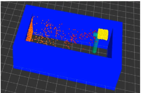
The first experiment was run in a rectangle shaped environment, discretized in voxels of 1 m each. The environment had an area of 11mx6m and was 5m high (see Fig 5.1). The gas source was placed at the position (2,2) and 3m high. The generated wind files simulated a wind flow along the U direction that ranged from 1.7m/s to 2m/s. The simulator ran for 300 snapshots, therefore 300 gas concentration samples were available for the execution of the bout detection.
Fig 5.1: First environment (11x6) where the bout count was tested in simulation. 5 5 6 9 9 4 4 8 8 9 5 6 8 8 9 5 4 8 5 5 1 20 3 21 20 32 1 30 19 22 2 1 21 22 5 31 28 25 22 2 0 32 27 29 18
By defining α=1−2∗τ 1
half∗Δt in the EWMA filter step of the bout detection
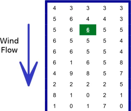
(equation 4.3) and computing the bouts in each cell it was seen that, contrary to expectations, the bout count doesn’t decrease with distance but rather increases (see Fig 5.2). 4 3 3 3 3 5 6 4 4 3 5 6 6 5 5 6 5 5 5 4 6 6 5 5 4 6 1 6 5 8 4 9 8 5 7 2 2 2 2 5 8 1 0 2 1 1 0 1 7 0
Fig 5.3: Results of the bout count in cells around the source in the environment presented in Fig 5.1. The green filled cell indicates the location of the source. The blue arrow represents the wind flow direction.
On the other hand by defining α=1−exp {log(0.5)
τhalf∗Δt} and using it in the EWMA
filter (equation 4.3), the bout count increased slightly for up to 4 meters from the source (see Fig 5.3). However, the changes in the number of bouts are almost negligible. The bout detection algorithm was designed to work on low wind speeds in the range of 0.1-0.3m/s, so the high wind speed could be a factor for not detecting any notable changes.
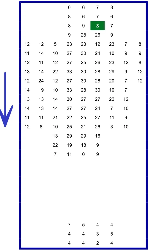
In the second simulation experiment a bigger environment (see Fig 5.4) was used (41mx16m). Because of the very long computation time, the concentration signal was built out of 150 simulation snapshots. The wind flows according to the U axis direction. The gas source was placed at the position (8, 10) and 3 meters above the ground.
Fig 5.4: Second environment (41x16) where the bout count was tested in simulation.
The wider area of the environment allows this experiment to show a more complete pattern of the number of bouts with respect to the distance from the source. It can be noticed that the bout count increases when moving away from the source for up to 6-7 meters before decreasing again gradually. After 12-13 meters the effect of the gas plume on the bout count seems to vanish.
5.2 Bout detection results in real world experiments
Several experiments were held in real world environments. The robot was equipped with six SGX MOX sensors (described in Chapter 3) configured with the respective approximate resistor loads:S1 S2 S3 S4 S5 S6
R (kOhm) 10 1 1 4 12 1
6 6 7 8 8 6 7 6 8 9 8 7 9 28 26 9 12 12 5 23 23 12 23 7 8 11 14 10 27 30 24 10 9 9 12 11 12 27 25 26 23 12 8 13 14 22 33 30 28 29 9 12 12 24 12 27 30 28 20 7 12 14 19 10 33 28 30 10 7 13 13 14 30 27 27 22 12 14 13 14 27 27 24 7 10 11 11 21 22 25 27 11 9 12 8 10 25 21 26 3 10 13 29 29 16 22 19 18 9 7 11 0 9 7 5 4 4 4 4 3 5 4 4 2 4
Fig 5.5: Results of the bout count in some cells around the source in the environment presented in Fig 5.4. The green filled cell indicates the location of the source. The blue arrow represents the wind flow
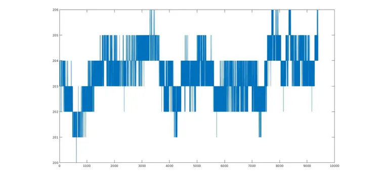
The gas plume was generated through evaporation of propanol from a small container. In order to generate the wind flow a fan was used that blew towards the robot. The bout detection was tested on low wind speeds (0.1m/s and 0.3m/s). The container was placed in between the robot and the fan in different distances from the robot in the range from 2 to 4 meters. The sampling rate of the sensors was set to 74 Hz and the sensing time of the robot was 135 seconds, obtaining gas concentration signal with a total of 10000 samples for the bout detection algorithm. The bout count was computed individually for each sensor.
Fig 5.8: Plot of the bout count results from the first experiment with 0.3m/s wind
Fig 5.6: Plot of the bout count results from the first experiment with 0.1m/s wind speed
Fig 5.7: Plot of the bout count results from the second experiment with 0.1m/s wind speed
Fig 5.9: Plot of the bout count results from the second experiment with 0.3m/s wind
From the different experiments that were held, in simulation and in the real world it can be said that the bout count gives mixed results in open environments. In some cases (such as from the signal of the S5 sensor in the first test at 0.1m/s wind), instead of decreasing as we would expect, the bout count increases with distance. In other cases, the bout count changes isn't related to the distance at all, giving mixed results that would make it useless for the purpose of estimating the location of the gas source. This can be typically seen in the response of the S2 and S3 sensors at 0.3m/s wind conditions. Detailed results are presented in Appendix B.
From the analysis of the gas concentration signal, however, it could be noted that there is another pattern in the bout detection that can potentially be used for estimating the gas source distance. In general, the amplitude of the bouts tends to decrease with distance, making it possible to estimate the distance to the source more accurately. In the experiments in the real world, the bout amplitude was computed for each sensor as the mean value of the amplitudes of all the bouts.
Fig 5.10: Plot of the bout amplitude results of the first experiment with 0.1m/s wind speed
Fig 5.11: Plot of the bout amplitude results from the second experiment with 0.1m/s wind speed
From the results it can be seen that, although not very robustly, the average bout amplitude is a good indicator of the distance to the gas source. We can see that the sensors with lowest resistor loads are more sensible to the distance than the other ones. The average bout amplitude is not very accurate in estimating the source distance within the range of 0.5m, meaning that in some sensors responses, when moving away from the source the amplitude sometimes slightly increases. However in most cases, the average bout amplitude decreases when moving away from the source for more than 1m. This makes it useful to mobile robotic olfaction applications in open environments.
The bout detection algorithm was tested in outdoor environments also, but with no promising results. The wind flow conditions are not stable in outdoor environments which results in the wind changing direction very often. Moreover, the wind speed is in general much higher than in indoor environments. In the experiment that was held the wind speed was in the range of 1 m/s which makes the bout detection algorithm useless. The average bout amplitude was very low and practically indistinguishable from the blank case.
Fig 5.13: Plot of the bout amplitude results from the second experiment with 0.3m/s wind speed
5.3 Exploration results
The exploration algorithm was tested on the Husky A200 physical platform, produced by Clearpath Robotics. Besides the six SGX MOX sensors on an Arduino board, the robot was equipped with a Windsonic sensor produced by Gill Instruments Ltd. In order to build the map of the environment and determine the obstacles' distance from the robot a Light Detection and Ranging (LIDAR) sensor was mounted on the base platform.
The environment on which the robot performed the exploration was setup on the Teknikhuset corridor at the Örebro University. The environment used was about 22 meters long and 4 meters wide.
To simulate gas leaks, a container filled with propanol was placed on a table and the gas plume was created through evaporation. The fan placed on the table near the gas source is used to simulate a wind flow. Different experiments were held by positioning the fan in order to generate wind flows with different directions and different wind speeds.
Fig 5.14: Husky A200 (Clearpath Robotics) equipped with a Windsonic sensor, MOX sensors and the LIDAR scanner
Fig 5.15: Teknikhuset corridor at the Örebro University where the experiments were held
In all experiments, the robot was placed on the start position on the west point as indicated in the environment map. The obstacles introduced in the map represent the location of the table where the gas source is placed and the presence of stairs in the corridor. Although these obstacles are clearly marked in an occupancy grid, in order to properly avoid them the robot keeps a certain distance from them. This is achieved by inflating these obstacles in the occupancy grid according to the robot's size.
The sensory function for Gaussian Regression was derived from the bout amplitudes of the signals of each sensor. As it can be seen from the results of the source distance estimation, the bout amplitude indicator is not very robust. The estimation of the source distance wouldn't always be accurate if it were to be derived from a single sensor, especially in high wind speeds. The low resistance sensors are highly sensitive and not very reliable. The bout amplitude from the high resistance
sensors, on the other hand, shows slight changes with distance. Therefore, the distance was estimated by a contribution of each sensor. More specifically, for each sensing operation, the average bout amplitude for each sensor was calculated first and then the six values are averaged together to have the final value. In this way, the effect of the very sensitive sensors is attenuated by the others in order to give a good estimation. The map for navigation purposes was discretized in cells of one meter per side because of the robot’s size. On the other hand, the mean estimation and variance maps computed from Gaussian Regression are discretized in cells of ten centimeters per side each in order to have a finer grid of values.
a)
In Fig 5.17, the mean estimation and variance maps computed by Gaussian Regression at the end of execution are represented, considering the average bout amplitude as the sensory function. In this scenario, the fan placed on the table was oriented towards the stairs in order to have a southeast direction for the wind. The robot’s sensing time was set to 135 seconds, which correspond to 10000 samples of gas concentration. In the mean map, the dark blue regions represent low values of the
b)
c)
Fig 5.17: Results from the first experiment. Wind flows towards the south-east direction. Sensing time is 135 seconds a) the mean map: light blue regions indicate a high mean value. b) the variance map: yellow
the origin, then the final chosen position was in coordinates (9, 0) which is located immediately south of the table. If we consider also the inflation of the obstacles for navigation purposes, then this final position that was chosen is actually the closest reachable position to the gas source. It is noteworthy to mention that at the beginning of the execution, the robot made a broad exploration of the environment (on the west side). By the end of the execution, the robot instead of exploring further in the east side, it chose positions near the table, which are located in the upwind direction. As expected, the robot tends to prefer exploration in the beginning of the execution and slightly move towards exploitation by the end of it.
In Fig 5.18, the mean and variance maps represent the results of another experiment in which the fan was oriented towards the starting position of the robot and so the wind was flowing towards the south-west direction. In this experiment, the robot’s sensing time was set to 67 seconds which correspond to 5000 samples of gas concentration. The area in the west side of the map, where the gas was flowing, is marked in light blue to indicate high bout amplitude values. Although the overall light blue area is not very accurate in indicating the positions near the source, in the end the
Fig 5.18: Mean and variance map of the second experiment. Wind flows towards the south-east direction. Sensing time is 67 seconds. a) the mean map: light blue regions indicate a high mean value.
b) the variance map: yellow regions indicate low variance c) the red circle indicates the final position a)
b)
robot chose the position (5, 1) as the nearest one to the source. This position is located in fact immediately in the south-west direction of the source and is the location where the highest bout amplitude was measured. By analyzing the variance map it can be seen that the robot after making a broad exploration in the west side, by the end of the algorithm decided to just go upwind (in the east direction).
In Fig 5.19, the mean map of the same scenario as in Fig 5.18 is represented, but doubling the sensing time. With a longer sensing time, the robot was able to identify the more accurately the areas near the gas source. However, in both cases, the robot in the end chose the same cell as the final position nearest to the source.
Fig 5.19: Mean map of the third experiment. Wind flows towards the south-west direction. Sensing time is 135 seconds.
In Fig 5.20, an experiment with higher wind speed is represented. In this scenario, the wind speed was about 1 m/s. The wind was flowing towards the south-west direction. Unfortunately, the bout detection algorithm is not reliable in high wind speeds. The maximum speed of operation is in the range 0.3-0.4 m/s. As a result, although the robot went near the source during the exploration, the highest bout amplitude was measured near the starting position, thus failing to find the gas source.