An evaluation of feature matching strategies for visual tracking

(1)

POLITECNICO DI MILANO Facolta di Ingegneria dell'Informazione

POLO REGIONALE DI COMO

Corso di Laurea Specialistica in Ingegneria Informatica

AN EVALUATION OF FEATURE

MATCHING STRATEGIES FOR

VISUAL TRACKING

Supervisor: Prof. Matteo MATTEUCCI Master Thesis of: Arash MANSOURI Matriculation: 735043

(2)

An Evaluation of Feature Matching Strategies for Visual Tracking

2

3

7.1.5 5th Test - ROI group points ... 68

7.2 Set B ... 70

7.2.1 6th Test – Total Point to Point-2frames ... 71

7.2.2 7th Test - ROI Points 2frames ... 76

7.3 Set C ... 80

8 Discussion, Conclusion and Future Development ... 81

(4)

4

(5)

5

(6)

6 3 Feature Detection and Detectors

3.1 Introduction

In this chapter, the definition and algorithm of detectors which are used in this work will be explained. First an introduction to the definition of feature is given and then ―Kanade-Lucas-Tomasi‖ detector, ―Harris detector‖ and ―Fast-Hessian‖ detector which are used in this work will be simply presented.

3.2 Definition of a Feature

Let’s say that there is not a certain and exact definition for what constitutes a feature. This definition is strongly related to the problem and type of the image application. But generally it could be defined that a feature illustrates ―interesting‖ part of an image and they are used as a starting point for many computer vision algorithms. Feature detection is a low-level image processing operation and they are used as the starting point and main primitives for subsequent algorithms so it shows how much this starting part could be essential for overall algorithm. Many computer vision algorithms use feature detection as the initial step, so as a result, a very large number of feature detectors have been developed. These vary widely in the kinds of feature detected, the computational complexity and the repeatability.

A local feature is an image pattern which differs from its immediate neighborhood. It is usually associated with a change of an image property or several properties simultaneously, although it is not necessarily localized exactly on this change. The image properties commonly considered are intensity, color, and texture. Figure below shows some examples of local features in a contour image (left) as well as in a gray value image (right). Local features can be points, but also edgels or small image patches. Typically, some measurements are taken from a region centered on a local feature and converted into descriptors. The descriptors can then be used for various applications.

(7)

7

Figure. Importance of corners and junctions in visual recognition and an image example with interest points provided by a corner detector

3.2.1 Image Feature Types

We could sort some type of image feature as following: Edges

Edges are points where there is a boundary (or an edge) between two image regions. In general, an edge can be of almost arbitrary shape, and may include junctions. In practice, edges are usually defined as sets of points in the image which have a strong gradient magnitude.

Corners

The terms corners and interest points are used somewhat interchangeably and refer to point-like features in an image, which have a local two dimensional structure. The name "Corner" arose since early algorithms first performed edge detection, and then analyzed the edges to find rapid changes in direction (corners). These algorithms were then developed so that explicit edge detection was no longer required, for instance by looking for high levels of curvature in the image gradient. It was then noticed that the

(8)

8

so-called corners were also being detected on parts of the image which were not corners in the traditional sense (for instance a small bright spot on a dark background may be detected). These points are frequently known as interest points, but the term "corner" is used by tradition.

Blobs / regions of interest or interest points

Blobs provide a complementary description of image structures in terms of regions, as opposed to corners that are more point-like. Nevertheless, blob descriptors often contain a preferred point (a local maximum of an operator response or a center of gravity) which means that many blob detectors may also be regarded as interest point operators. Blob detectors can detect areas in an image which are too smooth to be detected by a corner detector.

3.2.2 Feature detector categorization base on their application

In the following, we distinguish three broad categories of feature detectors based on their possible usage. It is not exhaustive or the only way of categorizing the detectors but it emphasizes different properties required by the usage scenarios:

1. One might be interested in a specific type of local features, as they may have a specific semantic interpretation in the limited context of a certain application. For instance, edges detected in aerial images often correspond to roads; blob detection can be used to identify impurities in some inspection task; etc. These were the first applications for which local feature detectors have been proposed. 2. One might be interested in local features since they provide a limited set of well

localized and individually identifiable anchor points. What the features actually represent is not really relevant, as long as their location can be determined accurately and in a stable manner over time. This is for instance the situation in most matching or tracking applications, and especially for camera calibration or 3D reconstruction.

(9)

9

3. A set of local features can be used as a robust image representation that allows recognizing objects or scenes without the need for segmentation. Here again, it does not really matter what the features actually represent. They do not even have to be localized precisely, since the goal is not to match them on an individual basis, but rather to analyze their statistics.

So as it was mentioned, each of the above three categories imposes its own constraints, and a good feature for one application may be useless in the context of a different problem.

Notice: Interest Point and Local Feature

In a way, the ideal local feature would be a point as defined in geometry: having a location in space but no spatial extent. In practice however, images are discrete with the smallest spatial unit being a pixel and discretization effects playing an important role. To localize features in images, a local neighborhood of pixels needs to be analyzed, giving all local features some implicit spatial extent. For some applications (e.g., camera calibration or 3D reconstruction) this spatial extent is completely ignored in further processing, and only the location derived from the feature extraction process is used (with the location sometimes determined up to sub-pixel accuracy). In those cases, one typically uses the term interest point.

3.2.3 Properties of a Ideal Local Feature

Followings are some properties of a Local Feature:

 Repeatability: Given two images of the same object or scene, taken under

different viewing conditions, a high percentage of the features detected on the scene part visible in both images should be found in both images.

 Distinctiveness/in formativeness: The intensity patterns underlying the

detected features should show a lot of variation, such that features can be distinguished and matched.

(10)

10

 Locality: The features should be local, so as to reduce the probability of

occlusion and to allow simple model approximations of the geometric and photometric deformations between two images taken under different viewing conditions (e.g., based on a local planarity assumption).

 Quantity: The number of detected features should be sufficiently large, such

that a reasonable number of features are detected even on small objects. However, the optimal number of features depends on the application. Ideally, the number of detected features should be adaptable over a large range by a simple and intuitive threshold. The density of features should reflect the information content of the image to provide a compact image representation.

 Accuracy: The detected features should be accurately localized, both in

image location, as with respect to scale and possibly shape.

 Efficiency: Preferably, the detection of features in a new image should allow

for time-critical applications.

Repeatability, arguably the most important property of all, can be achieved in two different ways: either by invariance or by robustness.

 Invariance: When large deformations are to be expected, the preferred

approach is to model these mathematically if possible, and then develop methods for feature detection that are unaffected by these mathematical transformations.

 Robustness: In case of relatively small deformations, it often suffices to

make feature detection methods less sensitive to such deformations, i.e., the accuracy of the detection may decrease, but not drastically so. Typical deformations that are tackled using robustness are image noise, discretization effects, compression artifacts, blur, etc. Also geometric and photometric deviations from the mathematical model used to obtain invariance are often overcome by including more robustness.

(11)

11

Clearly, the importance of these different properties depends on the actual application and settings, and compromises need to be made.

Repeatability is required in all application scenarios and it directly depends on the other properties like invariance, robustness, quantity etc. Depending on the application increasing or decreasing them may result in higher repeatability.

Distinctiveness and locality are competing properties and cannot be fulfilled simultaneously: the more local a feature, the less information is available in the underlying intensity pattern and the harder it becomes to match it correctly, especially in database applications where there are many candidate features to match to. On the other hand, in case of planar objects and/or purely rotating cameras, images are related by a global homography, and there are no problems with occlusions or depth discontinuities. Under these conditions, the size of the local features can be increased without problems, resulting in a higher distinctiveness.

Similarly, an increased level of invariance typically leads to a reduced distinctiveness, as some of the image measurements are used to lift the degrees of freedom of the transformation. A similar rule holds for robustness versus distinctiveness, as typically some information is disregarded (considered as noise) in order to achieve robustness. As a result, it is important to have a clear idea on the required level of invariance or robustness for a given application. It is hard to achieve high invariance and robustness at the same time and invariance, which is not adapted to the application, may have a negative impact on the results.

Accuracy is especially important in wide baseline matching, registration, and structure from motion applications, where precise correspondences are needed to, e.g., estimate the epipolar geometry or to calibrate the camera setup.

Quantity is particularly useful in some class-level object or scene recognition methods, where it is vital to densely cover the object of interest. On the other hand, a high number of features have in most cases a negative impact on the computation time and it should be kept within limits. Also robustness is essential for object class recognition, as it is impossible to model the intra-class variations mathematically, so full invariance is impossible. For these applications, an accurate localization is less important. The effect of inaccurate localization of a feature detector can be countered, up to some point, by

(12)

12

having an extra robust descriptor, which yields a feature vector that is not affected by small localization errors.

3.3 Harris Detector

The Harris detector, proposed by Harris and Stephens, is based on the second moment matrix, also called the auto-correlation matrix, which is often used for feature detection and for describing local image structures. This matrix describes the gradient distribution in a local neighborhood of a point:

With

The local image derivatives are computed with Gaussian kernels of scale (the differentiation scale). The derivatives are then averaged in the neighborhood of the point by smoothing with a Gaussian window of scale (the integration scale). The eigen values of this matrix represent the principal signal changes in two orthogonal directions in a neighborhood around the point defined by . Based on this property, corners can be found as locations in the image for which the image signal varies significantly in both directions, or in other words, for which both eigen values are large. In practice, Harris proposed to use the following measure for cornerness, which combines the two eigen values in a single measure and is computationally less expensive:

(13)

13

with the determinant and the trace of the matrix . A typical value for λ is 0.04. Since the determinant of a matrix is equal to the product of its eigen values and the trace corresponds to the sum, it is clear that high values of the cornerness measure correspond to both eigenvalues being large. Adding the second term with the trace reduces the response of the operator on strong straight contours.

Subsequent stages of the corner extraction process are illustrated in Figure :

Fig. Illustration of the components of the second moment matrix and Harris cornerness measure.

Figure ?? shows the corners detected with this measure for two example images related by a rotation. Note that the features found correspond to locations in the image showing two dimensional variations in the intensity pattern. These may correspond to real ―corners‖, but the detector also fires on other structures, such as T-junctions, points with high curvature and etc.

(14)

14

Fig. Harris corners detected on rotated image examples.

As can be seen in the figure, many but not all of the features detected in the original image (left) have also been found in the rotated version (right). In other words, the repeatability of the Harris detector under rotations is high. Additionally, features are typically found at locations which are informative, i.e., with a high variability in the intensity pattern. This makes them more discriminative and easier to bring into correspondence.

3.4 Hessian Detector

The second matrix issued from the Taylor expansion of the image intensity function is the Hessian matrix:

with etc. second-order Gaussian smoothed image derivatives. These encode the shape information by describing how the normal to an isosurface changes. As such, they capture important properties of local image structure. Particularly interesting are the filters based on the determinant and the trace of this matrix. The latter is often referred to as the Laplacian. Local maxima of both measures can be used to detect blob-like structures in an image The Laplacian is a separable linear filter and can be approximated efficiently with a Difference of Gaussians (DoG) filter. The Laplacian filters have one

(15)

15

major drawback in the context of blob extraction though. Local maxima are often found near contours or straight edges, where the signal change is only in one direction.

These maxima are less stable because their localization is more sensitive to noise or small changes in neighboring texture. This is mostly an issue in the context of finding correspondences for recovering image transformations. A more sophisticated approach, solving this problem, is to select a location and scale for which the trace and the determinant of the Hessian matrix simultaneously assume a local extremum.

This gives rise to points, for which the second order derivatives detect signal changes in two orthogonal directions. A similar idea is explored in the Harris detector, albeit for first-order derivatives only.

The feature detection process based on the Hessian matrix is illustrated in Figure ????. Given the original image (upper left), one first computes the second-order Gaussian smoothed image derivatives (lower part), which are then combined into the determinant of the Hessian (upper right).

Fig. Illustration of the components of the Hessian matrix and Hessian determinant.

The interest points detected with the determinant of the Hessian for an example image pair are displayed in Figure ????. The second-order derivatives are symmetric filters,

(16)

16

thus they give weak responses exactly in the point where the signal change is most significant. Therefore, the maxima are localized at ridges and blobs for which the size of the Gaussian kernel matches by the size of the blob structure.

Fig. Output of the Hessian detector applied at a given scale to example images with rotation (subset).

3.5 Kanade-Lucas-Tomasi Detector

The KLT algorithm is one of the selected detectors which are used in this work. In this section the definition of KLT feature detector is explained in detail but briefly, good features are located by examining the minimum eigenvalue of each 2 by 2 gradient matrix. In this method, it was shown how to monitor the quality of image features by using a measure of feature dissimilarity that quantifies the change of appearance of a feature between the first and the current frame. The idea is straightforward: dissimilarity is the feature’s rms residue between the first and the current frame and when dissimilarity grows too large the feature should be abandoned.

Basic requirements for KLT

As the camera moves, the patterns of image intensities change in a complex way. These changes can often be described as image motion:

(17)

17

Thus,a later image taken at time can be obtained by moving every point in the current image, taken at time , by a suitable amount. The amount of motion is called the displacement of the point at .

An affine motion field is a better representation: Where

is a deformation matrix, and is the translation of the feature window’s center.The image coordinates are measured with respect to the window’s center. Then,a point in the first image moves to point in the second image J,where and 1 is the identity matrix:

Because of image noise and as the affine motion model is not perfect, above equation is in general not satisfied exactly. The problem of determining the motion parameters is then that of finding the and that minimize the dissimilarity:

Where is the given feature window and is a weighting function. To minimize the residual of above equation we should differentiate it with respect to the unknown entries of the deformation matrix and the displacement vector and set the result to zero. We then linearize the resulting system by the truncated Taylor expansion:

This yields the following linear system:

Where collects the entries of the deformation

(18)

18

can be written as :

Z would be vital for our next calculation in good feature detection of KLT. For further information on and please refer to the reference paper.

In the KLT algorithm, they propose a more principled definition of feature quality. For selecting the reliable feature the symmetric matrix Z of the system must be both above the image noise level and well-conditioned.

The noise requirement implies that both eigen values of Z must be large, while the conditioning requirement means that they cannot differ by several orders of magnitude. Two small eigen values mean a roughly constant intensity profile within a window. A large and a small eigen value correspond to a unidirectional texture pattern. Two large eigen values can represent corners, salt-and-pepper textures, or any other pattern that can be tracked reliably.

In practice, when the smaller eigen value is sufficiently large to meet the noise criterion, the matrix Z is usually also well conditioned. In fact, the intensity variations in a window are bounded by the maximum allowable pixel value. so that the greater eigenvalue cannot be arbitrarily large. In conclusion, if the two eigenvalues of Z are

and ,we accept a window if

where is a predefined threshold.

It would be nice if we notice that a feature with a high texture content, as defined in the above equation, can still be a bad feature to track.For instance,in an image of a tree, a horizontal twig in the foreground can intersect a vertical twig in the background. This intersection occurs only in the image- not in the world- since the two twigs are at different depths. Any selection criterion would pick the intersection as a good feature to

(19)

19

track, and yet there is no real world feature there to speak of. The measure of dissimilarity defined in equation can often indicate that something is going wrong. Because of the potentially large number of frames through which a given feature can be tracked, the dissimilarity measure would not work well with a pure translation model.

(20)

20 4 Descriptors

4.1 Introduction

Interesting points on the object can be extracted to provide a "feature description" of the object. This description, extracted from a training image, can then be used to identify the object when attempting to locate the object in a test image containing many other objects. Image matching is a fundamental aspect of many problems in computer vision, including object or scene recognition, solving for 3D structure from multiple images, stereo correspondence, and motion tracking. A ―Descriptor‖ describes image features that have many properties that make them suitable for matching differing images of an object or scene. That features could be invariant to image scaling and rotation, and partially invariant to change in illumination and 3D camera viewpoint. To perform reliable recognition, it is important that the features extracted from the training image are detectable even under changes in image scale, noise and illumination. Such points usually lie on high-contrast regions of the image, such as object edges. More than above, relative positions between them in the original scene shouldn't change from one image to another. For example, if only the four corners of a door were used as features, they would work regardless of the door's position; but if points in the frame were also used, the recognition would fail if the door is opened or closed. Similarly, features located in articulated or flexible objects would typically not work if any change in their internal geometry happens between two images in the set being processed.

The following section will introduce two powerful descriptors - Scale-invariant feature transform and speed up robust features- in detail. The speed up robust features (SURF) is one which is implemented and used in this work as a descriptor.

4.2 SIFT: Scale-invariant feature transform

According to David Lowe, Following are the major stages of computation used to generate the set of image features:

1. Scale-space extrema detection: The first stage of computation searches over all scales and image locations. It is implemented efficiently by using a

(21)

difference-An Evaluation of Feature Matching Strategies for Visual Tracking

21

of-Gaussian function to identify potential interest points that are invariant to scale and orientation.

2. Keypoint localization: At each candidate location, a detailed model is fit to determine location and scale. Keypoints are selected based on measures of their stability.

3. Orientation assignment: One or more orientations are assigned to each keypoint location based on local image gradient directions. All future operations are performed on image data that has been transformed relative to the assigned orientation, scale, and location for each feature, thereby providing invariance to these transformations.

4. Keypoint descriptor: The local image gradients are measured at the selected scale in the region around each keypoint. These are transformed into a representation that allows for significant levels of local shape distortion and change in illumination.

This approach has been named the Scale Invariant Feature Transform (SIFT), as it transforms image data into scale-invariant coordinates relative to local features.

Detection of scale-space extrema

The first stage of keypoint detection is to identify locations and scales that can be assigned in a repeatable manner under differing views of the same object. The scale space of an image is defined as a function , that is produced from the convolution of a variable-scale Gaussian, , with an input image, :

where * is the convolution operation in and , and

Using scale-space extrema in the difference-of-Gaussian function convolved with the image, :

(22)

22

From above equation we could reach to following approximation (the proof is described in the reference [Distinctive Image Features from Scale-Invariant Keypoints,by david Lowe]) :

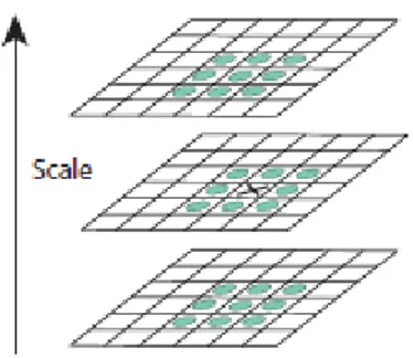
Where is scale-normalized Laplacian of Gaussian. This shows that when the difference-of-Gaussian function has scales differing by a constant factor it already incorporates the scale normalization required for the scale-invariant Laplacian. The factor in the equation is a constant over all scales and therefore does not influence extrema location. An efficient approach to construction of is shown in Figure ???. The initial image is incrementally convolved with Gaussians to produce images separated by a constant factor k in scale space, shown stacked in the left column.

Figure ????: For each octave of scale space, the initial image is repeatedly convolved with Gaussians to produce the set of scale space images shown on the left. Adjacent Gaussian images are subtracted to produce the difference-of-Gaussian images on the right. After each octave, the Gaussian image is

(23)

23

Local extrema detection

In order to detect the local maxima and minima of , each sample point is compared to its eight neighbors in the current image and nine neighbors in the scale above and below. It is selected only if it is larger than all of these neighbors or smaller than all of them. The cost of this check is reasonably low due to the fact that most sample points will be eliminated following the first few checks. (see figure 2???)

An important issue is to determine the frequency of sampling in the image and scale a domain that is needed to reliably detect the extrema. Unfortunately, it turns out that there is no minimum spacing of samples that will detect all extrema, as the extrema can be arbitrarily close together. Therefore, we must settle for a solution that trades off efficiency with completeness.

Figure 2: Maxima and minima of the difference-of-Gaussian images are detected by comparing a pixel (marked with X) to its 26 neighbors in 3x3 regions at the current and adjacent scales (marked with

circles).

Accurate keypoint localization

Once a keypoint candidate has been found by comparing a pixel to its neighbors, the next step is to perform a detailed fit to the nearby data for location, scale, and ratio of principal curvatures. This information allows points to be rejected that have low contrast (and are therefore sensitive to noise) or are poorly localized along an edge. Implementing of the above approach leads to

(24)

24

where and its derivatives are evaluated at the sample point and is the offset from this point. The location of the extremum, , is determined by taking the derivative of this function with respect to and setting it to zero, giving

The function value at the extremum, , is useful for rejecting unstable extrema with low contrast. This can be obtained by substituting two above, giving

Eliminating edge responses

For stability, it is not sufficient to reject keypoints with low contrast. The difference-of- Gaussian function will have a strong response along edges, even if the location along the edge is poorly determined and therefore unstable to small amounts of noise.

The first step here, is computing The principal curvatures from a 2x2 Hessian matrix, , computed at the location and scale of the keypoint:

The derivatives are estimated by taking differences of neighboring sample points. Now, Let be the eigenvalue with the largest magnitude and be the smaller one. Then, we can compute the sum of the eigenvalues from the trace of H and their product from the determinant:

Now, Let be the ratio between the largest magnitude eigenvalue and the smaller one, so that Then by some calculation we could reach to:

So it shows that this quantity is at a minimum when the two eigenvalues are equal and it increases with .

(25)

25

Orientation assignment

By assigning a consistent orientation to each keypoint based on local image properties, the keypoint descriptor can be represented relative to this orientation and therefore achieve invariance to image rotation. This approach contrasts with the orientation invariant descriptors of Schmid andMohr (1997), in which each image property is based on a rotationally invariant measure. The disadvantage of that approach is that it limits the descriptors that can be used and discards image information by not requiring all measures to be based on a consistent rotation.

Following experimentation with a number of approaches to assigning a local orientation, the following approach was found to give the most stable results. The scale of the keypoint is used to select the Gaussian smoothed image, , with the closest scale, so that all computations are performed in a scale-invariant manner. For each image sample at this scale, the gradient magnitude, , and orientation, , is pre-computed using pixel differences:

The local image descriptor

The previous operations have assigned an image location, scale, and orientation to each keypoint. These parameters impose a repeatable local 2D coordinate system in which to describe the local image region, and therefore provide invariance to these parameters. The next step is to compute a descriptor for the local image region that is highly distinctive yet is as invariant as possible to remaining variations, such as change in illumination or 3D viewpoint. One obvious approach would be to sample the local image intensities around the keypoint at the appropriate scale, and to match these using a normalized correlation measure. However, simple correlation of image patches is highly sensitive to changes that cause misregistration of samples, such as affine or 3D viewpoint change or non-rigid deformations. A better approach has been demonstrated by Edelman, Intrator, and Poggio (1997). Their proposed representation was based upon

(26)

26

a model of biological vision, in particular of complex neurons in primary visual cortex. These complex neurons respond to a gradient at a particular orientation and spatial frequency, but the location of the gradient on the retina is allowed to shift over a small receptive field rather than being precisely localized. Edelman et al. hypothesized that the function of these complex neurons was to allow for matching and recognition of 3D objects from a range of viewpoints. They have performed detailed experiments using 3D computer models of object and animal shapes which show that matching gradients while allowing for shifts in their position results in much better classification under 3D rotation.

Descriptor representation

First the image gradient magnitudes and orientations are sampled around the keypoint location, using the scale of the keypoint to select the level of Gaussian blur for the image. In order to achieve orientation invariance, the coordinates of the descriptor and the gradient orientations are rotated relative to the keypoint orientation. A Gaussian weighting function with equal to one half the width of the descriptor window is used to assign a weight to the magnitude of each sample point. The purpose of this Gaussian window is to avoid sudden changes in the descriptor with small changes in the position of the window, and to give less emphasis to gradients that are far from the center of the descriptor, as these are most affected by misregistration errors.

The keypoint descriptor allows for significant shift in gradient positions by creating orientation histograms over 4x4 sample regions. It is important to avoid all boundary affects in which the descriptor abruptly changes as a sample shifts smoothly from being within one histogram to another or from one orientation to another. Therefore, trilinear interpolation is used to distribute the value of each gradient sample into adjacent histogram bins. In other words, each entry into a bin is multiplied by a weight of for each dimension, where is the distance of the sample from the central value of the bin as measured in units of the histogram bin spacing.

The descriptor is formed from a vector containing the values of all the orientation histogram entries, corresponding to the lengths of the arrows.

Finally, the feature vector is modified to reduce the effects of illumination change. First, the vector is normalized to unit length. A change in image contrast in which each pixel

(27)

27

value is multiplied by a constant will multiply gradients by the same constant, so this contrast change will be canceled by vector normalization. A brightness change in which a constant is added to each image pixel will not affect the gradient values, as they are computed from pixel differences. Therefore, the descriptor is invariant to affine changes in illumination. However, non-linear illumination changes can also occur due to camera saturation or due to illumination changes that affect 3D surfaces with differing orientations by different amounts. These effects can cause a large change in relative magnitudes for some gradients, but are less likely to affect the gradient orientations. You can find all the above explanation in figure ???:

Figure ???: A keypoint descriptor is created by first computing the gradient magnitude and orientation at each image sample point in a region around the keypoint location, as shown on the left. These are weighted by a Gaussian window, indicated by the overlaid circle. These samples are then accumulated into orientation histograms summarizing the contents over 4x4 subregions, as shown on the right, with the

length of each arrow corresponding to the sum of the gradientmagnitudes near that direction within the region. This figure shows a 2x2 descriptor array computed from an 8x8 set of samples, whereas the

(28)

28

(29)

29 5 Evaluation and Statistics Definitions

5.1 Epipolar Geometry and the Fundamental Matrix

According to Richard Hartley in ―Multiple view geometry in computer vision‖ chapter 9, the epipolar geometry is the intrinsic projective geometry between two views.

It is independent of scene structure, and only depends on the cameras internal parameters and relative pose. Suppose a point in 3-space is imaged in two views, at in the first, and in the second. As shown in figure ???? the image points and , space point X, and camera centers C are coplanar and lie on a plane π, called the epipolar plane. Moreover we may define the baseline as the line joining the two camera centers and the epipole as the point of intersection of the line joining the camera centers (the baseline) with the image plane. Equivalently, the epipole is the image in one view of the camera center of the other view.

Figure???: The two cameras are indicated by their centers and and image planes. The camera centers, 3-space point , and its images and lie in a common plane π. An image point x back-projects to a ray in 3-space defined by the first camera center, , and . This ray is imaged as a line in the second view. The 3-space point which projects to must lie on this ray, so the image of in the second view must

(30)

30

Supposing now that we know only , we may ask how the corresponding point in the second view is constrained. See figure ????above: the epipolar plane is determined by the baseline and the ray defined by . From above we know that the ray corresponding to the (unknown) point lies in π, hence the point lies on the line of intersection of π with the second image plane.

This line is the image in the second view of the ray back-projected from . It is the epipolar line corresponding to . Thus there is a mapping to that can be represented in a 3x3 matrix F such that:

As we are dealing with geometric entities that are expressed in homogeneous coordinates. This representation permits to write a simple equation to determine if a point lies on a line , that is

From above we have that the point in the first view correspond to in the second view, and must lie on the epipolar line . So we can write:

Using in the last equation leads to the most basic properties of the fundamental matrix F that is:

This is true, because if points and correspond, then lies on the epipolar line corresponding to the point . In other words . Conversely, if image points satisfy the relation then the rays defined by these points are coplanar. This is a necessary condition for points to correspond. Note that, geometrically, represents a mapping from the 2-dimensional projective plane of the first image to the pencil of epipolar lines through the epipole on the second image. Thus it represents a mapping from a 2-dimensional onto a 1-dimensional projective space, and hence must have rank 2. Moreover, we emphasize the fact that the fundamental matrix is an homogeneous quantity, so it is defined up to a scale factor.

(31)

31

Now, Given sufficiently point correspondences (more than 7 points), this equation can be used to compute the unknown matrix . To explain this, we write , and

If we explicit the product in for a point correspondence we end up with this equation:

If we denote by f the 9-vector made up of the entries of in row-major order then above equation can be expressed as a scalar product:

From a set of points correspondences, we obtain a set of linear equations of the form:

This is a homogeneous set of equations and can only be determined up to scale. Now, for a solution to exist, matrix must have rank at most 8, and if the rank is exactly 8, then the solution is unique (up to scale). Please note that a solution for homogeneous linear system of the form is a vector in the so called nullspace of . The rank-nullity theorem states that the dimensions of the rank and the nullspace add up to the number of columns of . Matrix in above matrix has 9 columns so when its rank is 8 the nullspace is composed by only one vector , that is the unique solution.

Obviously the data correspondences will not be exact because of noise and the rank of may be greater or lower than 8. In the former case the nullspace is empty, so the only solution one can find is a least-squares solution. A method to obtain this

(32)

32

particular solution for , is to select the singular vector corresponding to the smallest singular value of .

The solution vector f is then the last column of in the .

As one can see, the matrix depends only on the points correspondences . Thus, its rank also will be conditioned by the point matches. There are cases in which these correspondences can lead to a matrix with rank less than 8, thus avoiding the existence of a unique solution (for instance when all the probing sources lie on a common plane, or a common line). In this case infact the nullspace of has dimension greater than 1, so a solution for above matrix is a linear combination of all the vectors in the nullspace For instance, when all the probing sources lie on a common plane, or a common line. Hence, it is important to choose the positions of the probing signals as random as possible within the field of view of the two acoustic cameras, in order to well condition the problem and avoid low rank problems.

5.2 Planar Homographies

Any two images of the same planar surface in space are related by a homography (assuming a pinhole camera model). This has many practical applications, such as image rectification, image registration, or computation of camera motion—rotation and translation—between two images. Once camera rotation and translation have been extracted from an estimated homography matrix, this information may be used for navigation, or to insert models of 3D objects into an image or video, so that they are rendered with the correct perspective and appear to have been part of the original scene. If the camera motion between two images is pure rotation, with no translation, then the two images are related by a homography (assuming a pinhole camera model).

(33)

33

Fig.

Consider a 3D coordinate frame and two arbitrary planes, The first plane is defined by the point and two linearly independent vectors , contained in the plane. Now, consider a point in this plane. Since the vectors and form a basis in this plane, we can express as:

Where defines the plane and defines the 2D coordinates of with respect to the basis

The similar identification is valid for the second plane

Where defines the plane while defines the 2D coordinates of with respect to the basis

By imposing the constraint that point maps to point under perspective projection, centered at the origin = , so

Where is a scalar that depends on , and consequently on . Combining the equation above with the constraint that each of the two points must be situated in its

(34)

34

corresponding plane, one obtains the relationship between the 2D coordinates of these points:

Note that the matrix A is invertible because are linearly independent and nonzero (the two planes do not pass through origin). Also note that the two vectors and above have a unit third coordinate. Hence the role of is simply to scale the term _{such that its third coordinate is 1. But, we can get rid of this}

nonlinearity by moving to homogeneous coordinates:

Where h h are homogeneous 3D vectors. _{is called a homography matrix}

and has 8 degrees of freedom, because it is defined up to a scaling factor ( where is any arbitrary scalar).

Applications of Homographies

Here are some computer vision and graphics applications that employ homographies:

 mosaics (image processing):

Involves computing homographies between pairs of input images Employs image-image mappings

 removing perspective distortion (computer vision)

Requires computing homographies between an image and scene surfaces Employs image-scene mappings

 rendering textures (computer graphics)

Requires applying homographies between a planar scene surface and the image plane, having the camera as the center of projection

Employs scene-image mappings

 computing planar shadows (computer graphics)

Requires applying homographies between two surfaces inside a 3D scene, having the light source as the center of projection

(35)

35

Now, under homography, we can write the transformation of points in 3D from two cameras (camera 1 to camera 2) as:

In the image planes, using homogeneous coordinates, we have

This means that is equal to up to a scale (due to universal scale ambiguity). Note that is a direct mapping between points in the image planes. If it is known that some points all lie in a plane in the first image, the image can be rectified directly without needing to recover and manipulate 3D coordinates.

Homography Estimation

To estimate , we start from the equation . Written element by element, in homogenous coordinates we get the following constraint:

In inhomogeneous coordinates :

In this work, we set the ,actually without loss of generality:

(36)

36 5.3 Generalized Extreme Value Distributions

Extreme value theory is a separate branch of statistics that deals with extreme events. This theory is based on the extremal types theorem, also called the three types theorem, stating that there are only three types of distributions that are needed to model the maximum or minimum of the collection of random observations from the same distribution.

According to Samuel Kotz and S. Nadarajah, Extreme value distributions are usually considered to comprise the following three families:

Type 1, (Gumbel-type distribution):

Type 2, (F'rCchet-type distribution):

Type 3, (Weibull-type distribution):

The generalized extreme value (GEV) distribution was first introduced by Jenkinson (1955).The cumulative distribution function of the generalized extreme value distributions is given by

(37)

37

It has also the following PDF:

where , and k, , are the shape, scale, and location parameters respectively. The scale must be positive ( ), the shape and location can take on any real value. The range of definition of the GEV distribution depends on k:

Various values of the shape parameter yield the extreme value type I, II, and III distributions. Specifically, the three cases k=0, k>0, and k<0 correspond to the Gumbel, Fréchet, and "reversed" Weibull distributions. The reversed Weibull distribution is a quite rarely used model bounded on the upper side. For example, for k=−0.5, the GEV PDF graph has the form:

(38)

38

When fitting the GEV distribution to sample data, the sign of the shape parameter k will usually indicate which one of the three models best describes the random process we are dealing with.

5.4 Goodness of Fit Test

The goodness of fit (GOF) tests measures the compatibility of a random sample with a theoretical probability distribution function. In other words, these tests show how well the selected distribution fits to the data and our test condition and hypothesis will be described.

Anderson-Darling test

The Anderson-Darling procedure is a general test to compare the fit of an observed cumulative distribution function to an expected cumulative distribution function. This test gives more weight to the tails. In this section, the definition of this test is explained in detail.

Anderson and Darling (1952, 1954) introduced the goodness-of-fit statistic

to test the hypothesis that a random sample , with empirical distribution , comes from a continuous population with completely specified distribution function .Here is defined as the proportion of the sample that is not greater than . The corresponding two-sample version

was proposed by Darling (1957) and studied in detail by Pettitt (1976). Here is the empirical distribution function of the second (independent) sample obtained from a continuous population with distribution function , and , with , is the empirical distribution

(39)

39

function of the pooled sample. The above integrand is appropriately defined to be zero whenever .

The k-sample Anderson-Darling test is a rank test and thus makes no restrictive parametric model assumptions. The need for a k-sample version is twofold. It can either be used to establish differences in several sampled populations with particular sensitivity toward the tails of the pooled sample or it may be used to judge whether several samples are sufficiently similar so that they may be pooled for further analysis. According to F. W. Scholz and M. A. Stephens (Sep.1987); Let be the th observation in the th sample ). All observations are independent. Suppose that the th sample has continuous distribution function . We wish to test the hypothesis

without specifying the common distribution . Denote the empirical distribution function of the th sample by and that of the pooled sample of all

observations by . The k-sample Anderson-Darling test statistic is then defined as:

where . Under the continuity assumption on the the probability of ties is zero. Hence the pooled ordered sample is , and a straightforward evaluation of above equation yields the following computational formula for : kN _N _n i NMij jni j N j N j k i

where M_ij is the number of observations in the ith sample that are not greater than _j. In our test in this work, The Anderson-Darling statistic ( ) is simply defined as:

(40)

40

Hypothesis Testing

The null and the alternative hypotheses are:

 : the data follow the specified distribution;

 : the data do not follow the specified distribution.

The hypothesis regarding the distributional form is rejected at the chosen significance level ( ) if the test statistic, , is greater than the critical. The fixed values of (0.01, 0.05 etc.) are generally used to evaluate the null hypothesis ( ) at various significance levels. In general, critical values of the Anderson-Darling test statistic depend on the specific distribution being tested but the value of 0.05 is used for most tests.

The Anderson-Darling test implemented in this work uses the same critical values for all distributions. These values are calculated using the approximation formula, and depend on the sample size only. This kind of test (compared to the "original" A-D test) is less likely to reject the good fit, and can be successfully used to compare the goodness of fit of several fitted distributions.

(41)

41 6 Proposed Methods

6.1 Tracking Methods

Total Comparison Point to Point Method

In this method, we start with the first frame at time ( ). The detection algorithm is run on the whole frame and all the features are detected in the first frame . Then all these extracted features are passed to the descriptor with the needed parameters and so the descriptor is ready to describe each extracted point based on information on detector. It means that the features of frame are now completely detected and described in all related parameters such as scale, distance, laplacian parameters and descriptor array.

After the previous stage, the same procedure is done for the second frame ( ) and all the features in that frame is extract and described for frame .

For matching step, in this method, each interest point in the frame will be compare with whole interest points from previous frame ‖Point to Point‖. The method is shown in the figure ???.

Fig.the left image is the frame and the green dots shows the interest points (note that in real algorithm these interest points are much more than above image). The right image is related to frame and the red line shows the

comparison method

In this method it is expected that we face to higher match points with higher calculation time which leads to lower frame per second value (fps).

(42)

42

Region of Interest (ROI) Point to Point Method

In this method, the procedure of loading and detecting the interest points are same. It means that the detecting algorithm is run on the whole starting frame and so the interest features are detected. Then the whole algorithm will be run on the second frame

and every interest points in this frame (current frame) will be described as well. On this method -as it arises from the name – a region will be defined around each interest point in . This region could be in different pixel size such as , or even . The region will be mapped accordingly from frame to and the size of the region will be strictly maintained. Then each interest points in frame will be compared with the corresponded features in the defined ROI on frame . This comparison will be point to point in the selected ROI. The figure ??? shows this method.

Fig. the left image shows the IPs in frame while the red square is mapped ROI from frame . The green dots are the IPs in both frames.

In this method it is expected that we face to lower match points in compare with previous method with lower calculation time which leads to higher frame per second value (fps).

(43)

43

Region of Interest (ROI) Group Centroid Comparison Method

As previous, the detection algorithm will be run on the whole frame in and all the features are detected in that frames, then the same algorithm will be run on the second frame and the interest points are described as well on that frame. Till this step it would be exactly same as the two previous methods.

Then the region of interest is defined around each IP in frame with the arbitrary size of , or . For comparison method, the selected ROI will be mapped accordingly in the frame with same size. In this step, we have a selected ROI with interest points inside the region on frame . In this method the centroid of these interest points are calculated from their descriptor parameters by simply making the average from each parameter. Then an virtual interest point will be created as well with new parameters from all IPs in selected ROI. The comparison will be done between the interest point in frame and the Centroid in frame . So the comparison will be just done between two points instead of . It means that in this procedure we will have comparison instead of . the figure ??? shows this method.

Fig. the left image shows the mapped ROI and its IPs. The orange dot shows the centroid of IPs in selected ROI.

In this method it is expected that we face to more match points in compare with previous method with more or less the same calculation time. So the matched points will be increased in this method.

(44)

44

Total Comparison Point to Point Method with Two Frames

In this method the whole algorithm is run on the frame and the interest points are detected and described. Then the whole algorithm for detecting and describing is run on the second frame as well but unlike the three previous methods, this is not the point of comparison. The detecting and describing algorithm is run for third frame and all the interest points are extracted and describe. This would be the step of comparison between interest points. The procedure is as following; at first each interest points in frame (which is called as current frame) will be compared to all described interest points in previous frame , if the algorithm find any matching between the interest point of current frame and the previous frame so the point will be flagged as matched, otherwise, the current interest point in frame will be evaluated against all interest points in two-previous frame searching for any matches. If the point finds its match in whole interest points in two-previous frame it will be flagged as match as well. The interest point is called as not match if during these two frame it could not find any point that satisfy the threshold condition.

The figure ???? shows this algorithm. the left frame is frame , the middle and right frames are frames and respectively. The two detected IPs in frame illustrate the algorithm of matching in previous frame and two-previous frame. The continues black lines show matching in previous frame while the dash red lines shows not matching in previous frame and so the algorithm referral in two-previos frame for finding matches.

(45)

45

Region of Interest (ROI) Point to Point Method with Two Frames

In this algorithm, the procedure of running detection algorithm is same as previous method, it means the detection algorithm is run on the whole first frame and all the IPs are detected. The same procedure of detection IPs is run for the second and third frames as well ( ). Now the comparison stage is start. In this step, a region of interest (ROI) is drawn around each interest point in current frame . The size of this ROI could be selected from , or . After detecting this window, the algorithm maps exact size ROI on the two previous frames as well and the potential match points will be search in these ROI. The detail is as following; at first the algorithm search to find the match interest point in previous frame ROI. This matching search will be Point to Point in the selected ROI. It means the current frame IP will be evaluated against all IPs inside the previous ROI frame ( ) in terms of descriptors. If any IP in the ROI passed from matching threshold , the IP in current frame is flagged as match, otherwise, the two-previous frame will be evaluated in exactly mapped ROI. If the current frame IP is matched with any IP in frame , the current IP will be flagged as match and if there are not any interest points passed the matching threshold condition even in two-frame previous, then the current IP in frame

will be flagged as not matched.

The figure ??? shows the Region of Interest (ROI) Point to Point Method with Two Frames algorithm. The left frame is frame (the first frame), the middle and right frames are second and third frames ( ) respectively. The current two IPs in frame (right frame) will matched with previous and two-previous frames in black lines and red dash lines respectively.

(46)

46

Fig. Region of Interest (ROI) Point to Point Method with Two Frames algorithm

Region of Interest (ROI) Group Centroid Comparison Method with Two Frames In this method, the detection algorithm is run for first three frames separately and all the features are detected in each frame respectively. Note that this procedure is the same as above method in first step and it is not run simultaneously on three frames but frame by frame. After detecting IPs in each frame, the ROI will be selected around each feature in current frame which is in our example. Then the correspondence ROI will be mapped in previous frame and two-previous frame (frames respectively).

The difference of this method in compares with ―Region of Interest (ROI) Point to Point Method with Two Frames ―is based on their comparison method. In this method, the average of descriptor parameter will be calculated for all the IPs in mapped ROI in frames , and the virtual Centroid of these IPs will be compare with the current frame IP. It means that we will have comparison instead of . If the Centroid of group IP in selected ROI is matched with the current frame IP, so its flag will be changed to ―Matched‖ otherwise, the current frame IP must be evaluated with the Centroid of correspondence ROI in two-previous frame . If the comparison between this group Centroid in frame and the current frame IP in passed the threshold condition then the current frame IP flag will be change to matched and if non of the above condition were satisfied , then the Current frame IP will not be matched with any previous frames IP.

The figure??? Shows the algorithm. The left, middle and right frames are respectively. As it is shown, the orange points are the Centroid of group IP in selected ROI. If the Centroid satisfies the threshold condition in middle frame (the black line),