Analysis of urban metabolism and policy assessment : building a nested multiregional input-output model

(1)

1

POLITECNICO DI MILANO

Scuola di Ingegneria Industriale e dell’Informazione

Dipartimento di Energia

Master of Science in Energy Engineering

Analysis of urban metabolism and policy assessment:

building a Nested Multiregional Input-Output model

Supervisor:

Matteo Vincenzo Rocco

Thesis of: Alberto Brambilla di Civesio ID number 875699

Davide Buratti ID number 876521

(2)

2

List of figures

Figure 1 – Share of urban and rural population by region 1950-2050 ... Error!

Bookmark not defined.9

Figure 2 – Metric tons of CO2 emissions per capita and share of urban

population ... 10

Figure 3 – Global temperature anomaly 1920-2018 and future trend ... 11

Figure 4 – CO2 emissions trends in different policy scenarios ... 12

Figure 5 – Relative difference between CBA and PBA for 79 C40 cities ... 15

Figure 6 – Percentages of the main world economiess studied in the publications about urban and/or regional pollution ... 20

Figure 7 – Percentages of the frameworks utilized in the cited publications ... 22

Figure 8 – Percentages of the analysis methods utilizeed in the cited publications ... 23

Figure 9 – Percentages of the accounting methods used in the cited papers ... 24

Figure 10 – Pecentages of the types of indicators used in the literature ... 25

Figure 11 – Framework-Indicator Sankey diagram ... 26

Figure 12 – Basic structure of Leontief Input-Output model ... 31

Figure 13 – Basic Multiregional Input-Output framework ... 35

Figure 14 – Basic Nested Multiregional Input-Output model ... 44

Figure 15 – Resource/waste model for a generic production system ... 45

Figure 16 – Basic Environmental-Extended Input-Output table ... 47

Figure 17 – Estimation of intra- and interregional flows ... 55

Figure 18 – Parameters for the allocation of interregional flows ... 55

Figure 19 – Functional layout of the Python script ... 60

Figure 20 – Comparison between regional direct CO2 emissions obtained by model B and the ones of th Istat database ... 62

Figure 21 – Comparison between regional direct CO2 emissions obtained by model A and the ones of th Istat database ... 62

Figure 22 – Comparison of Mton of CO 2 emissions embodied in the flows of products for 6 regions for the four possible configurations of model B ... 63

Figure 23 – Comparison of Mton of CO 2 emissions embodied in the flows of products for 20 regions for the five possible configurations of model A ... 64

Figure 24 – Comparison of Mton of CO 2 emissions embodied in the flows of products for Milan for the five possible configurations of model A ... 65

Figure 25 – Comparison of Mton of CO 2 emissions embodied in the flows of products for Milan for the five possible configurations of model A ... 66

(5)

5

Figure 27 – Heat-map of intra- and interreginal carbon flow for model A ... 67

Figure 28 – Specific embodied CO2 emissions of region for model A ... 70

Figure 29 – Specific embodied CO2 emissions of region for model A ... 70

Figure 30 – Specific embodied CO2 emissions of region for model B ... 71

Figure 31 – Specific embodied CO2 emissions of region for model B ... 71

Figure 32 – Sectoral CO2 embodied emissions of Northern for model B ... 72

Figure 33 – Percentage of specific embodied sectoral emissions for ten pollutants for region Lombardy in model A ... 73

Figure 34 – Percentage of total embodied sectoral emissions for ten pollutants for region Lombardy in model A ... 74

Figure 35 – Carbon Footprint of Milan ... 75

Figure 36 – Total sectoral embodied carbon emission of Milan for model C ... 76

Figure 37 – Total sectoral embodied carbon emission of Milan for model B . Error! Bookmark not defined.7 Figure 38 – Specific sectoral embodied carbon emission of Milan for model C ... Error! Bookmark not defined. Figure 39 – Specific sectoral embodied carbon emission of Milan for model B .... 78

Figure 40 – Variation of sectoral value added of Milan ... 83

Figure 41 – Variation of sectoral Carbon Footprint of Milan ... 83

Figure 41 – Variation of specific sectoral Carbon Footprint of Milan ... 84

List of tables

Table 1 – Net CO2 importers and exporters in Italian context for model B... 67

Table 2 – Net CO2 importers and exporters in the international context for model B ... 68

Table 3 – Net CO2 importers and exporters in Italian context for model A ... 69

Table 4 – Sectoral distribution of specific and total costs associated to the application of the policy ... 80

Table 5 – Possible regional distribution of the costs associated to the application of the policy ... 81

Table 6 – Total production and carbon flow variations in case 1, 2 and 3 ... 82

Nomenclature

Notation

(6)

6 𝑎̂ Diagonalization of vector 𝑎

𝑎𝑇, 𝐴𝑇 Transposed vectors and matrices 𝐴−1 Inverse matrices

𝐼 Identity matrices

Acronyms

CBA Consumption-Based Accounting

EE-IOA Environmental-Extended Input-Output Analysis EET Emissions Embodied in Trade

GDP Gross Domestic Product

GHG Greenhouse Gasses

GPC Global Protocol for Community-Scale GHG emission Inventories GRP Gross Regional Product

ICLEI International Council for Local Environmental Initiatives IEA International Energy Agency

IO Input-Output

IOA Input-Output Analysis

IPCC Intergovernmental Panel on Climate Change LCA Life Cycle Assessment

MFA Material Flow Analysis

MIOT Monetary Input-Output Table MRIO Multiregional Input-Output

OECD Organization for Economic Cooperation and Development PBA Production-Based Accounting

SRIO Single Region Input-Output RoW Rest of the World

WRI World Resources Institute

Symbols

𝑥 Total production vector

𝑋 Total gross output

𝑓 Final demand vector

𝑍 Intermediate transactions matrix

𝐴, 𝑎𝑖𝑗 Technical coefficients matrix and technical coefficients 𝐿 Leontief inverse matrix

𝑅 Exogenous resources/wastes matrix

𝐵, 𝑏_𝑖𝑗 Input coefficients matrix and input coefficients 𝑒𝑒 Specific embodied exogenous resources matrix 𝐸𝐸 Embodied exogenous resources matrix

𝑉𝑎 Value added vector

𝑣 Value added coefficients vector

(7)

7

𝑒 Exports vector

Sommario

In accordo con le proiezioni dell’Intergovernmental Panel on Climate Change (IPCC), la limitazione del riscaldamento globale sotto 1.5 °C rispetto al livello preindustriale è strettamente collegata alla riduzione di emissioni di gas serra. Ad oggi più di metà della popolazione mondiale vive in zone urbane e le città contribuiscono circa al 75% delle emissioni di gas serra. Considerando che è previsto il raggiungimento del 68% di popolazione urbana entro il 2050, le città assumono un ruolo chiave nella lotta al cambiamento climatico. Infatti, in accordo con l’International Energy Agency (IEA), le aree urbane rappresentano due terzi del potenziale per ridurre efficientemente le emissioni globali di carbone in termini di costi. Alla base della lotta al cambiamento climatico, le città devono calcolare le loro emissioni di CO2 in modo efficace e completo. Il tradizionale Production-Based Accounting deve essere integrato con il Consumption-Based Accounting per valutare la “responsabilità” delle emissioni di CO2. I responsabili delle politiche devono essere informati tramite precise e specifiche analisi che sottolineino le connessioni intersettoriali all’interno e all’esterno dei confini cittadini. L’obiettivo di questo lavoro è lo sviluppo di un modello ambientale multiregionale Input-Output a tre livelli spaziali applicato all’Italia, alle sue regioni e all’area metropolitana di Milano. Il sistema è stato modellato a partire dai database Exiobase 3 e Istat, applicando metodologie tradizionali e revisionate di regionalizzazione e urbanizzazione dei dati. Il modello permette di calcolare, secondo una logica CBA, l’impronta di carbonio e i flussi di carbonio associati a 17 settori produttivi dell’economia italiana, regionale e dell’area metropolitana di Milano per analizzare come tali settori interagiscano l’uno con l’altro. I risultati ottenuti mostrano come il duplice scaling dei dati (da nazione a regione e da regione a città) dia una rappresentazione più realistica del sistema urbano rispetto a quella che si otterrebbe scalando i dati direttamente dalla dimensione nazionale a quella cittadina. In aggiunta all’analisi attributiva, è stato realizzata un’analisi consequenziale per una prima valutazione di impatto ambientale ed economico della politica sui tetti verdi contenuta nel nuovo Piano di Governo del Territorio di Milano (PGT).

(8)

8 Keywords: Analisi ambientale e multiregionale di Input-Output, Impronta di Carbonio, Flussi di Carbonio, Emissioni di CO2 “embodied", Metabolismo Urbano.

(9)

9

Abstract

According with the projections of the Intergovernmental Panel on Climate Change (IPCC), the limitation of global warming below 1.5 °C above pre-industrial level is strictly related to the reduction of GHG emissions. Nowadays, more than half of the world’s population lives in urban areas and cities contribute approximately to 75% of world’s GHG emissions. Considering that the share urban population is forecasted to reach 68% by 2050, cities will play a key role in the fight for climate change. Indeed, according to the International Energy Agency (IEA), urban areas account for up to two-thirds of the potential to cost-effectively reduce global carbon emissions. As a basis for action on climate change, cities should report their CO2 emissions in an effective and complete way. The traditional Production-Based Accounting should be integrated with the Consumption-Based Accounting to assess the “responsibility” of CO2 emissions. The policy-makers should be informed through precise and specific analysis highlighting the inter-sectoral connections arising inside and outside the city boundaries. The objective of this work is to develop a Nested Environmental-Extended Multiregional Input-Output (Nested EE-MRIO) model with three spatial levels, applied to Italy, Italian regions and the metropolitan area of Milan. The framework has been modeled through Exiobase 3 and Istat databases, applying traditional and modified methodologies of downscaling of data at regional and urban dimensions. The model estimates, according to a CBA logic, the Carbon Footprint and the carbon flows associated to 17 production sectors of Italy, of the Italian regions and of the metropolitan area of Milan, in order to analyse how these sectors interact with each other. The results show that the double scaling of data (from nation to region and then from region to city) gives a more realistic representation of the urban system than the one obtained by scaling directly national data to the urban dimension. The attributional analysis has been followed by a consequential analysis to give a first environmental and economic assessment of the green roofs policy that is included in the new Piano di Governo del Territorio (PGT) of Milan.

Keywords: Environmental-Extended Multiregional Input-Output Analysis, Carbon Footprint, Carbon Flows, Embodied CO2 emissions, Urban metabolism.

(10)

10

1. Introduction

1.1 Urbanization phenomenon and environmental pollution

of cities

The post-industrial society has been characterized by a steady shift from rural to urban living. Nowadays 55% of the world’s population lives in urban areas and, according to the World Urbanization Prospect published by the United Nations, this percentage is expected to reach a share of 68% by 2050 [1]. The OECD countries have shown this tendency since the half of the twentieth century, increasing their urban percentage from 56% to 80 % in the last seventy years. Despite this, a further increase of that share in developed countries is forecasted. Developing countries have subsequently followed the same path and nowadays their urbanization rate is faster compared to historical trends of OECD countries [1].

(11)

11 Metropolis are the poles of the process of centralisation, hosting a quarter of the world’s population. Generally, metropolitan areas tend to outperform in economic terms other areas of the same nation, showing a GRP (Gross Regional Product) above the national average [3]. A higher GRP is related with higher average income for people working in the region. Higher wages, better education and services the city can offer, attract people from other areas and foster the progressive transformation of rural areas into peripheral urban districts. In the years to come, metropolis will further expand and smaller cities will become metropolis as well. The massive demographic density, registered in the cities’ environment, goes hand in hand with a great resource consumption, both for public administration and for private use. Energy, regardless of the source, is the engine of all the activities of cities. It is needed for transport, buildings, infrastructures, industrial and commercial activities, water and food distribution. Cities account for about 70% of the world energy demand [4].

It is straightforward that a great consumption of energy and resources is related with high polluting emissions: economic growth and Greenhouse Gasses (GHG) emissions move in tandem. Urban residents and activities contribute approximately to 75% of global GHG emissions. There is a direct correlation between the level of urbanization and the metric tons of CO2 emissions per capita (Figure 2). According to the World Bank data, the higher is the percentage of urban residents on the total population, the higher are the CO2 emissions per capita.

Figure 2. Metric tons of CO2 emissions per capita and share of urban population [5]. Source:

(12)

12 In forecast of a worldwide increase of the share of urban population, a crucial target for policymakers is to reverse or at least stem this dangerous trend. Since most of the GHG emissions are concentrated in urban areas, cities have a key role in climate change. The fight for climate change has been one of the main global topics in the last years and it is going to play a central role in the national and international politics of the next decades. According to the Special Report [6] of 2018, carried out by the Intergovernmental Panel on Climate Change (IPCC), human activities are estimated to have caused 1.0°C of global warming above pre-industrial level. If current warming rate continues, the world would reach human-induced global warming of 1.5°C around 2040, causing impacts on human and natural systems. Adopting the Paris Agreement in 2015, for the first time governments from all over the world agreed to “hold the increase in the global average temperature well below 2 °C above pre-industrial levels and to pursue efforts to limit the temperature increase to 1.5 °C above pre-industrial levels, recognizing that this would significantly reduce the risks and impacts of climate change” [7].

Figure 3. Global temperature anomaly 1920-2018 and trend [8]. Source: Berkeley Earth.

The challenge that national governments are facing is pushing cities to play a dominant role in sustainable development and in climate change mitigation, because they have the potential to initiate low-carbon infrastructure pathways and influence changes in lifestyle. Indeed, according to the International Energy Agency

(13)

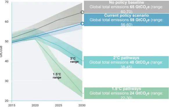
13 (IEA), urban areas account for up to two-thirds of the potential to cost-effectively reduce global carbon emissions. Building cities that are green, inclusive and sustainable should be the foundation of any local and national climate change agenda, because sustainable development can be built only upon sustainable cities. The world is urbanizing quickly and under the Current Policies Scenario (CPS), GHG emissions will keep increasing dramatically [9]. In contrast, global GHG emissions in 2030 need to be approximately 25 percent and 55 percent lower than in 2017 to put the world on a least-cost pathway to limiting global warming to 2 °C and 1,5 °C respectively.

Figure 4. CO2 emissions trends in different policy scenarios. Source: IPCC.

Cities are usually first-responders in a crisis; they are the first to experience trends, because of their proximity to the public and their commitment on providing day-to-day services. Cities governments tend to be more pragmatic than national ones. The target for the next years is to address global warming mitigation policies towards urban dimension instead of national dimension, in order to capture the variation of characteristics among different cities of the same country. The sustainability goals and the decarbonisation process should include all the metropolis, with a particular focus on the metropolis of developing countries, on the dominant world metropolis and on the metropolis of developed countries that

(14)

14 are experiencing a significant demographic and economic growth. These are the cities that are mostly able to make a difference by becoming an example and influencing the behaviour of the other cities. The infrastructure of 2050 is being built today, yet the world of 2050 will be very different from today.

1.2 Pollution as a multi-perspective issue

The last century has seen the spreading of another phenomenon besides the urbanization: the globalization. The whole of the world is increasingly behaving as it were a part of a single market, with interdependent production, consumption and demand of similar products and responding to the same impulses. Globalization is manifested in a huge amount of material goods traded by every country all over the world. According to the World Bank data, during the 20th century the ratio of world imports to gross world product has grown from 7% in 1938 to 13% in 1970 to over 20% at the end of the century. The percentage has reached a kind of plateau in the 21st_{century, settling in a range from 25% to 28%} [10]. The massive monetary flows associated with international trades are related with equally large GHG emissions embodied in the traded goods. With GHG embodied emissions of a product are indicated all the accumulated emissions emitted in the production and distribution of that product.

The “pollution heaven hypothesis” [11], which argues that developed countries are likely to transfer the polluting industry to developing countries that have lower environmental regulations, further justifies the embodied carbon’s crucial role in international carbon allocation.

As a basis for action on climate change, countries should quantify and report their GHG emissions. It is important that the accounting of GHGs emissions of nations is accurate, comparable and complete.

Typically, emissions statistics are compiled according to production‐based accounting (PBA), also defined as territorial-based accounting or sector-based accounting: it measures emissions occurring within sovereign borders. However, these estimates do not reflect production chains which extend across borders and, although this is the traditional accounting method, it is not effective in describing the real emissions attributable to a country.

A more holistic way of analysing the responsibility for GHG emissions is to compile statistics according to consumption-based accounting (CBA), which considers both direct and indirect emissions, the latter of which refers to the GHG that is embodied in the intermediate products and material that are passed on to other sectors until

(15)

15 they reach the final consumer. In simple terms, PBA allocates emissions to the local producers, while CBA allocates emissions to the final consumer rather than the producer.

The consideration of emissions embodied in trade (EET) may have a significant impact on participation in and effectiveness of global climate policies, particularly for three aspects. First, a direct analysis of EET provides a better understanding of the separation between domestic consumption and domestic production,

assessing the “responsibility” of pollution. Second, an analysis of carbon leakages reveals if pollution is shifted rather than abated. Third, trade-adjusted GHG emission inventories attempt to exploit trade to mitigate emissions.

Analysing the interconnections between countries could fill the lack of detailed knowledge about induced emissions occurring outside the country’s boundaries, but this is not sufficient for a comprehensive description of the system. Indeed, the analysis of spatial linkages should be followed by the unravelling of inter-sectoral linkages, in order to describe the complexity of interconnections between industries and regions located upstream or downstream the supply chain.

As said previously, more than half of the world’s population lives in cities, but cities’ surface is just the 3% of the earth’s surface [5]. Therefore, EET are even more impactful for cities than countries, because cities source a major part of their resource demand from their local, national and global hinterland, causing emissions across the whole global supply chain.

Several studies demonstrate that transboundary energy use in key infrastructures serving cities can usually be as large, or larger than the direct energy use and GHGs emissions within city boundaries [12].

To promote growth and also mitigate climate change, cities have to act on different aspects at the same time, without leaving none of them behind. Fiscal policy reform can create strong incentives for low-carbon investments and reducing GHG emissions. The use of carbon pricing is only emerging in many countries and generally not applied at a sufficient level to facilitate a shift towards low-carbon environments. Emission reduction potential from non-state and subnational action could be significant, allowing countries to achieve their targets, but the impact of pledged commitments are limited and poorly documented. Combining innovation in the use of existing technologies and in behaviour with the promotion of investment in new technologies and market creation has the potential to transform societies and reduce their GHG emissions. At the basis of these multi-perspective actions, cities as well as countries must quantify and report their GHG emissions. A

(16)

16 city consumption-based GHG inventory can be defined as the emissions arising within city’s boundaries, minus those emissions associated with the production of goods and services exported outside the city, plus emissions generated in the supply chains for goods and services produced outside the city but imported to meet the final demand of its residents. On the contrary, a city production-based GHG inventory can be defined as the emissions arising within city’s boundaries, plus those emissions associated with the production of goods and services exported outside the city. A positive difference between CBA and PBA values indicates that the city is a net importer of GHG emissions. Vice versa, a negative difference between CBA and PBA values indicates that the city is net exporter of GHG emissions.

Figure 5. Differences between consumption-based GHG inventories and production-based GHG inventories for 79 C40 cities [13]. Source: C40 Cities.

An accurate assessment of urban GHG emissions should take into account both methodologies of accounting. The reasons why current urban climate change

(17)

17 mitigation initiatives overwhelmingly focus on territorial emissions are both pragmatic and political. Local decision makers are often unaware of the relevance of upstream emissions. The literature on upstream urban emissions is sparse and comparisons among cities are hampered by differences in methods, classifications and terminology [14].

However, since ICLEI published in 2009 the first version of the Local Government GHG Analysis Protocol [15], several other guidelines and standards have been published to assist cities to account for their GHG emissions. The most advanced and recent standards to date are the PAS 2070 specification for the assessment of GHG emissions of a city, which has been developed by the World Resources Institute (WRI), C40 Cities Climate Leadership Group, and ICLEI–Local Governments for Sustainability. The Global Protocol for Community-Scale Greenhouse Gas Emission Inventories (GPC) distinguishes three scopes [16]. The scopes are the most used and standardized definition for classifying the direct and indirect emissions:

• Scope 1: direct GHG emissions from sources located inside the city boundary (direct emissions).

• Scope 2: direct GHG emissions caused by the use of grid-supplied electricity, heating and cooling inside the city boundary.

• Scope 3: GHG emissions occurring outside the city boundary for activities occurring inside the city boundary (other indirect emissions).

In this context, the understanding and the representation of the urban system complexity is the first key point to implement a specific and effective set of measures. The modeling of the urban structure should be capable of representing the specificities and the identity of the city. In this direction, it is fundamental to take into account strengths and weaknesses of its economic sectors, as well as the behaviour of its residents and the characteristics of the macro-region to which the city belongs. Nowadays, there is not a unified and standardized procedure of analysis of urban environmental impact, although the topic has been widely discussed and studied. Several analytical frameworks have been adopted to assess urban metabolism and these have be further discussed in the literature review (Chapter 2). Most of these analyses are carried out through proprietary software and not open datasets, making it difficult to understand the hypothesis at the base of the model and its building path. The absence of this information hampers the effectiveness of the comparison of results obtained with different models and the possibility to apply the same model to different systems.

(18)

18

1.3 Work objectives

The aim of this work is to develop a model that is able to achieve a comprehensive and deep analysis of the inter-sectoral and spatial linkages at urban, regional and national level. The model is applied to Italy and, since it utilizes public and free datasets, it is designed to be applicable to other nations by making few appropriate modifications. The urban analysis is carried out considering the metropolitan area of Milan, since it has a remarkable role in the Italian context and it is experiencing a rapid demographic and economic growth. The further development of the model is facilitated through the creation of an open-source Python script, which also permits a quick calculation of the results.

Spatial and sectoral interconnections are evaluated in a multidimensional way by considering both environmental and economic terms. It is crucial to characterize simultaneously the material and the monetary flows entering/exiting into regional and urban areas: how they are transformed by specific sectoral activities and how they impact on the environment through their consumption of resources and generation of wastes. The model is able to identify sectors and areas that need to be targeted in future interventions towards urban and regional decarbonisation, without hampering the economic dimension.

For what concerns the accounting methodology, the model can evaluate both consumption-based and production-based CO2 emissions, deepening results at multi-spatial and multi-sectoral levels. Considering both CBA and PBA perspective, it is possible for policy-makers to study in detail sectoral and spatial carbon flows and implement proper and effective policies to reduce the carbon emissions of cities.

The innovative aspect of this work is the combination of a multi-level analysis at spatial scale, which considers three dimensions in the scaling process (nation, region and metropolitan area). In this way, with the application of a dynamic analysis, it is possible to obtain two-ways results: how an urban policy may affect urban, regional and national spheres, and how a national policy can influence national, regional and urban contexts.

To reach the targets of the study, several publications have been selected and analysed to deepen into the topic and to select the proper model to be developed. The findings of the literature review are discussed in chapter 2. The basic analytical structure of the model is illustrated in chapter 3, while the practical application of

(19)

19 the model to our case is described in chapter 4. The results of the attributional and consequential analysis and the verification of the model are discussed in chapter 5.

(20)

20

2. Literature Review

The late 20th_{century and the beginning of the 21}st_{century have marked a turning} point in the awareness of how human activities affect local and global environment. Consequently, in the last years several studies have tried to evaluate the ecological role of cities, regions and nations and to estimate the scale of their impact. A critical review of scientific literature has been conducted, in order to understand in which direction the scientific community is moving towards. Articles regarding analytical frameworks and analysis adopted to deal with urban pollution and urban planning strategies were the main topics of research.

Papers, reports and web articles published from 2007 to 2019 have been collected from online catalogues (Scopus, Elsevier, etc.) and classified according to the following categories: • Year of publication • Title • Author • Journal of publication • Framework • Analysis method • Topic • Accounting system • Data source • Type of indicator • Boundaries of analysis

All the catalogued publications and the associated categories are listed in the table in the Appendix B.

In the section 2.1 the most interesting categories are examined in detail and in the section 2.2 are reported the conclusions regarding the critical analysis of the papers.

(21)

21

2.1 Critical analysis of the papers

2.1.1 Boundaries of analysis

Building a model for the study of regional and urban behaviour is strictly possible if there is a sufficient availability of detailed data. The collection of a great amount of data is a very expensive and complex operation. For this reason, almost the entire literature is focused on the most developed countries.

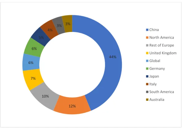
China, that is the largest GHG emitter in the world with nearly 10 billion tons of CO2 emissions (28% of global emissions in 2015) [17], has attracted the interest of researchers, being the subject of 44% of the considered publications.

The other world powers, such as the North America and the major European countries, are splitting the remaining share (39%) of the analysed papers, leaving a slight percentage to Japan (5%) and Australia (3%).

There are also other publications, defined with “Global” (6%) that analyse the relationships between all countries with a multi-regional model, without focusing on a particular country.

Figure 6. Percentages of the main world economies studied in the publications about urban and/or regional pollution.

44% 12% 10% 7% 6% 6% 5% 4% 3% 3% China North America Rest of Europe United Kingdom Global Germany Japan Italy South America Australia

(22)

22

2.1.2 Framework

Framework is defined as the analytical structure of the tool used to analyse the system. National, regional and urban environmental assessments are multidimensional and complex, therefore currently there is not a consensual method adopted. The authors choose the most suitable framework according to the target of the study and the availability of data.

Input-Output Framework

The Input-Output framework (IO) is a quantitative economic model that represents a national or regional economy by linking the different sectors of that particular economy. It shows the interdependencies between different sector, depicting how output from one sector becomes an input to another one and vice versa.

In a system with n sectors, the inter-industry matrix (n x n) is composed by column values and row values. Typically, column values represent input from the all sectors to a particular sector, while row values represent outputs from a given sector to the all other sectors.

When the framework is built for a single region, it is defined as Single Region Input-Output model (SRIO). IO models for different regions can be aggregated to investigate spatial linkages within countries besides sectoral linkages: the resulting system is called Multi-regional Input-Output model (MRIO).

Life Cycle Assessment

Life Cycle Assessment (LCA) is a technique used to evaluate environmental impacts related to the whole life of a product. This framework is generally built with a bottom-up approach, differently from the IO model, that usually makes use of a top-down approach.

The LCA model considers all the steps of the product’s life, starting from raw material extraction, passing through material processing, manufacture, distribution, use, repair and ending with disposal or recycling.

This structure is very efficient for a critical analysis of a specific product or sector, but it results too detailed and difficult to implement for the study of all the sectors of a country’s economy.

Material Flow Analysis

Material Flow Analysis (MFA) is an analytical framework used to quantify stocks of materials or substances and flows across different industrial sectors or within

(23)

23 ecosystems. It is a tool to study the biophysical aspects of human activity on different spatial and temporal scales. MFA can be applied, depending on the purpose of the study, to a specific industrial installation or to a wider system as long as it is well defined.

Network Model

The network model is a quantitative framework used to predict a number of interesting urban or regional phenomena. It can be useful to explain the importance of particular junctions in transportation networks, the flow of traffic on city streets, the distribution of industry, services and retail establishments in urban or regional environments.

Most spatial network studies use to represent networks with two types of network elements: nodes and edges. Edges typically represent territorial segments, and nodes the junctions where two or more edges intersect. The analysis results illustrate the degree to which an edge or node is spatially connected to the surrounding path network.

Hybrid Frameworks

In the literature, hybrid models are defined as frameworks that are built by making use of two or more different types of framework. In our critical review, we found that the 8% of the publications rely on a hybrid IO-LCA model, which is developed by combining an IO structure with data derived with an LCA approach.

Figure 7. Percentages of the frameworks utilized in the cited publications.

46% 24% 8% 5% 6% 5% 6% MRIO SRIO Hybrid IO-LCA MFA LCA Others Network Model

(24)

24

2.1.3 Analysis Method

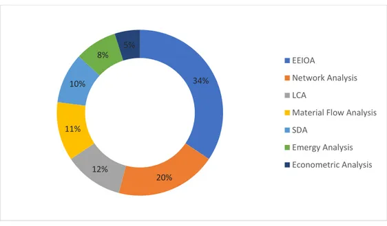
Once the framework is built, the model can be used to perform a deep analysis of the considered system. Several types of analysis follow different methodologies and give coherent results for the identified targets of the study. Most of those methods require very detailed data and are suitable for a focus on a specific industry, process or supply-chain.

When the willing of the publication is to investigate a wider and more complex system, like the entire economy of a region or a city and its interconnection with other economies, the most used techniques of analysis are the Environmental Extended Input-Output Analysis (34%) and the Emergy Analysis (8%).

The Environmental Extended Input-Output Analysis (EE-IOA) is performed by adding additional vectors to the traditional IO framework. Those vectors contain the quantitative amounts of resources/wastes that are directly absorbed/produced by all the sectors.

The Emergy Analysis evaluates all the work given by the environment to sustain a system and produce a certain level of output. Each form of energy in a system is translated into its solar energy equivalent, by multiplying its inputs and outputs for their respective solar transformities, which assess the energy’s qualitative value. Once calculated the amounts of each element of the system, those can be compared by means of emergy related ratios and indices, revealing the characteristics of the system in terms of efficiency and sustainability.

Figure 8. Percentages of analysis methods utilized in the cited publications.

34% 20% 12% 11% 10% 8% 5% EEIOA Network Analysis LCA

Material Flow Analysis SDA

Emergy Analysis Econometric Analysis

(25)

25

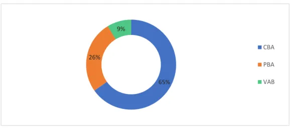
2.1.4 Accounting system

To support effective climate action planning, GHG accounting frameworks should: • Include both direct and indirect GHG emissions

• Provide sufficient detail to identify those sectors, processes and supply chains that have the largest potential for emission reductions

• Clearly identify the origin (location and industry or activity) of emissions • Allow for consistent benchmarking and comparisons

• Apply internationally recognized environmental and economic accounting principles

Despite the traditional accounting principle is the Production-Based Accounting (PBA), only the 26% of the considered publications actually use it. This is due to the large amount of imports that play an important role in almost all the economies of the world, especially for cities.

In order to evaluate carbon leakages, Consumption-Based Accounting (CBA), which is used in the 65% of the considered publications, fully counterbalances the unilateral responsibility of the producer for the pollution inherent to the production of a good that is consumed elsewhere.

The third accounting method found in the analysed literature is the Value-added Based Accounting (VBA). As the CBA it takes account of the carbon leakage, considering the emissions hidden in the value-added gained by the producers through the supply chain. Due to very detailed data needed for the VBA method, it is very complex to calculate and it has been adopted only in the 9% of the considered publications.

Figure 9. Percentages of accounting methods utilized in the cited papers

65% 26% 9% CBA PBA VAB

(26)

26

2.1.5 Indicators

Once the framework is built and the analysis is performed, the results have to be pointed out through appropriate and significative indicators, in order to obtain a successful description of the system.

We found in the literature that the 54% of the indicators in the considered papers are just environmental, while the 43% of them takes into account more than one dimension, in particular the 26% are environmental-economic indicators and the 17% are environmental-energy indicators.

Figure 10. Percentages of the types of indicator used in the literature.

Using multidimensional indicators, gives a more complete and detailed analysis of a system, but it is not always possible to have a multidimensional result, because it depends on the framework and the analysis method. Therefore, we built a Sankey diagram to visualize which frameworks are the most appropriate to provide multidimensional indicators.

The Sankey diagram shows that MRIO and SRIO models are those that present the larger use of multidimensional indicators, due to its structure that permits a direct link between monetary flows and GHG emissions’ flows. A multidimensional indicator can pinpoint crucial sectors that need to be targeted in future investments towards decarbonisation to minimise emissions and to maximise positive economic effects for urban and regional economies.

54% 26% 17% 3% Environmental Environmental-Economic Environmental-Energy Energy

(27)

27 Figure 11. On the left side of the Sankey diagram are reported the frameworks utilized in the considered publications, while on the right side are reported the mono- and multi-dimensional indicators used in the same papers. The width of the flows connecting the left nodes with the right

ones is proportional to the number of frameworks that provide the related indicator.

2.2 Results of the literature review

After an accurate and deep review of the literature, the most important conclusion is that the great amount of studies applies environmentally extended IO analysis to estimate environmental and economic indicators, due to the comprehensiveness of the model.

The 24% of the authors used the SRIO framework. It combines a good description of inter-industry linkages with a not excessive analytic complexity, but it assumes that imported goods and services are produced with the same technology of the domestic sector. Since the MRIO framework considers regional differences in production efficiency and tracks the supply chain, it has increasingly been adopted (46%) for global, national and sub-national studies, despite its more complex analytic structure.

We have identified that the type of model to implement, in order to obtain a sectoral and spatial analysis of Italy with a zoom on the city of Milan, is the Multi-Regional Input-Output model, because of its capability in capturing the linkages between sectors and regions. MRIO framework does not depend on defining system boundaries, thus it avoids truncation errors [18]. Moreover, with the

(28)

28 Environmental-Extended Input-Output Analysis, it is possible to provide multidimensional indicators that give environmental and economic measures. In the end, this framework allows us to account the GHG emissions with both the traditional Production-Based approach and the Consumption-Based approach. The double possibility of accounting is important in order to assess if a country, a region or a city, are net importers or exporters of GHG emissions.

(29)

(30)

30

3. Methods and models

The large production of goods and services by industrial and human activities is sustained by a flow of resources that may be coming from the environment, as raw materials, or from other processes, as intermediate products. Therefore, the assessment of resources and wastes consumed or rejected by a process, strongly depends on the behaviour of other processes belonging to the same system. In order to analyse a system, it is crucial to understand how its partitions interact with each other.

Once defined the kind of resources and wastes to be accounted for, time span and sectoral boundaries have to be established, according to the purpose of the analysis. Inputs and outputs of every sub-level of the system have to be reported using the same unit of measure, allowing for coherent comparisons and significant evaluations.

In the following paragraph 3.1, it is described in detail the basic analytic structure of a Regional Input-Output framework, the assumptions behind it and its multiregional developments. In paragraph 3.2 are depicted the procedures and techniques used to build a Multiregional Input-Output Table. Paragraphs 3.3 and 3.4 concern the merging of urban-level data in the structure and the rationale of the environmental extension of the system.

3.1 Input-Output Analysis: the basic framework

In 1973 Professor Wassily Leontief received the Nobel Prize in Economic Science in recognition of the development, in the late 1930s, of an analytic framework that took the name of Input-Output analysis. Nowadays the ideas behind the work of Leontief are key concepts of many system-analysis and, indeed, Input-Output is one of the most applied analysis methods. Born as a purely economic tool, IO analysis has developed and its applications have been extended to employment and social accounting metrics associated with industrial production, as well as to the energy consumption and environmental pollution accounting related with international and interregional inter-industry activities.

Generally, an Input-Output model is constructed using observed data of monetary transactions in a defined time span for a specific region of interest (nation, state, county, province, etc.). It is preferable to use monetary terms instead of physical

(31)

31 terms, because measurement problems could arise for industries that actually sell different types of goods.

The economic activity in the region is disaggregated in an arbitrary number of sectors. The level of the sector disaggregation depends on the availability of detailed data and the objectives that the model is expected to achieve. Considering a region with 𝑛 sectors, the associated IO table is depicted in Figure 12.

The part of the table coloured in yellow is the Intermediate transaction matrix 𝑍, wherein are reported the monetary transaction flows from each sector, considered as a producer, to each of the sectors, itself and the others, considered as consumers.

The first column of matrix 𝑍 is filled with the monetary flows associated to the physical input of intermediate products needed by sector 1 to produce its output and purchased from all the other sectors. Conversely, the upper row of matrix Z is filled with the monetary flows associated to the physical input of intermediate products needed by all the sectors to produce their outputs and purchased from sector 1. The diagonal elements of the matrix 𝑍 are the monetary flows associated to the physical amounts of intermediate products that are produced and consumed by the sectors themselves to produce their own outputs and are called intra-industry transactions.

The blue matrix is the Value-Added Matrix 𝑉𝑎 and accounts for the other inputs to production, such as non-industrial inputs (labour, depreciation of capital, taxes) and inputs coming from other regions, labelled as Imports.

The green portion of the table is the Final Demand Matrix 𝑓 and records the sales of each sector to final markets. In particular are reported households and governmental expenditures, as well as gross private investments and the exports to other regions.

(32)

32 Figure 12. A basic structure of Leontief Input-Output model, constituted by three matrices: the Intermediate transaction Matrix Z (yellow), the Value-Added Matrix (blue) and the Final Demand

Matrix (green).

The mathematical structure of a 𝑛 sector system consists of a set of 𝑛 linear equations. If we designate as 𝑧𝑖𝑗 the elements of the transaction matrix 𝑍, as 𝑥𝑖 the total output of sector 𝑖 and as 𝑓𝑖 the total final demand for sector 𝑖’s products, the distribution of sector 𝑖’s sales to other sectors and to final demand can be written as follow:

𝑥𝑖 = 𝑧𝑖1+ 𝑧𝑖𝑗+ . . . + 𝑧𝑖𝑛+ 𝑓𝑖 = ∑𝑛𝑗=1𝑧𝑖𝑗 + 𝑓𝑖 (3.1) There is an equation like this that identifies the distribution of the sales for each sector and all of them can be summarized in matrix notation (3.3), defining the total production vector 𝑥 (𝑛 x 1), the intermediate transaction matrix 𝑍 (𝑛 x 𝑛) and the final demand vector 𝑓 (𝑛 x 1) obtained as the sum of row elements of the finald demand matrix. 𝑥 = [ 𝑥_𝑖 … 𝑥𝑛 ] , 𝑍 = [ 𝑧₁₁ ⋯ 𝑧_1𝑛 ⋮ 𝑧_𝑖𝑖 ⋮ 𝑧_𝑛1 ⋯ 𝑧_𝑛𝑛] , 𝑓 = [ 𝑓_𝑖 … 𝑓_𝑛 ] (3.2) 𝑥 = 𝑍𝐼 + 𝑓 (3.3) In the equation 3.3, 𝐼 is used to represent a column vector of 1 of appropriate dimension (𝑛 x 1 in this case), that is called “summation vector”. The multiplication

(33)

33 for 𝑍 creates a column vector whose elements are the sums of the rows of the matrix.

Summing down the total output column, the result is the total gross output, 𝑋, throughout the economy. This same value can be found by summing across the total outlays row.

The contribution of a generic sector 𝑖 to the total output of a generic sector 𝑗 is defined by the technical coefficient 𝑎𝑖𝑗 = 𝑧𝑖𝑗⁄ , that measures the intermediate 𝑥𝑗 inputs needed by sector 𝑗 from sector 𝑖 to produce a single unit of product. Technical coefficents can be calculated for each couple of sectors and are depicted in the technical coefficient matrix 𝐴 (𝑛 × 𝑛).

In a generic IO model, a fundamental assumption is that the inter-industry flows of products from sector 𝑖 to sector 𝑗 are entirely dependent on the total output of the sector 𝑗. The fact that, for example, the more cars are produced in a year, the more steel will be needed by the cars’ producers during this year is a fair assumption. Some arguments may arise when technical coefficients 𝑎𝑖𝑗 are considered as fixed relationships between sectors, because economies of scales are not considered and production in a Leontief system operates under constant returns to scale.

The intermediate transaction matrix can be expressed as a function of the technical coefficient matrix 𝑍 = 𝐴𝑥̂, where 𝑥̂ is a diagonal matrix filled with the values of the total production vector 𝑥. Then the equation 3.3 can be written in a compact form:

𝑥 = 𝐴𝑥𝑖 + 𝑓 → 𝑥 = (𝐼 − 𝐴)−1𝑓 → 𝑥 = 𝐿𝑓 (3.4) 𝐿 is defined as the Leontief inverse Matrix or the total requirements matrix and is the core of the Input-Output framework. Each element of 𝐿 represents the embodied amount of input from sector 𝑖 required by the sector 𝑗 to produce one unit of its product as final demand.

Originally, applications of Input-Output model were performed at national levels and their main target was to assess the role of the different industrial sectors among the national economy. Over time, an additional interest regarding the inter-industry dynamics of a specific portion of national territory has risen, pushing the Input-Output analysis towards regional level. In order to reflect the peculiarities of a subnational system, the original Input-Output framework has been modified. Firstly, the structure of production may be identical or it may differ noticeably from that recorded in the national Input-Output table. Secondly, it is generally verified that small areas are more dependent than big areas on external trades, both for sales of regional outputs and purchases of imports needed for production.

(34)

34 In the following paragraphs will be examined the attempts that have been made to include the regional characteristics into an Input-Output framework, both for a single-region case and for a two or more-region case.

3.1.1 Regional Input-Output Table

Generally, single-region Input-Output analysis aims at quantifying the role of the producing sectors in that region and examining in detail the physiognomy of a particular region with respect to the nations to which it belongs. Moreover, several studies at regional level attempt to quantify, with a dynamic analysis, the impact on the sectors caused by a change of the regional final demand.

In order to perform those studies, two paths can be followed:

• Use a national table of technical coefficients jointly with an adjustment procedure designed to translate regional final demands into outputs of regional firms, since there is not a table of regional technical coefficients. The techniques used to “regionalize” national tables are described in detail in section 3.2.

• Build a regional model by surveying firms in the region and constructing a survey-based regional Input-Output table, based on true relationships between the regional sectors and not on estimations. Although this is the more precise of the two ways, the procedure of data collection is very expensive both in cost and time terms.

Single-region models fail to recognize what are the operative interconnections between different regions. The analysed region is “disconnected” from the rest of its home country, while in practice a number of important questions have several-region implications, because each of several-regional activities is expected to have trade relationships not only within the region where the activity takes place, but also to branch out towards other regions.

3.1.2 Multi-Regional Input-Output Table

In a many-regions Input–Output model (figure 13), the part of final demand that represents sales of sector 𝑖 to the productive sectors in other regions (but not to consumers in the other region) is removed from the voice “export” of final demand category and specified explicitly in the transaction matrix.

(35)

35 The fundamental problem in a many-regions Input-Output model is the description of the transactions between regions. One approach, the interregional model, considers a complete and ideal set of intra- and interregional data. It is never the case, in practice, that such a model can be implemented, due to the magnitude and the difficulty of the collection of the data needed. Indeed, the requirements grow more than linearly with the number of the regions in the model: a three-region model has six interregional matrices, a four-region model has twelve, and so on. Alternative many-regions Input-Output models have been developed and the most widespread in the literature is the Multiregional Input Output (MRIO) framework, due to an optimal trade-off between complexity of implementation and deepness of analysis. The MRIO model uses a regional technical coefficients matrix 𝐴𝑟, filled by regional technical coefficients 𝑎_𝑖𝑗𝑟, that respond to the question “How much sector 𝑖 product did you buy yearly to produce a unit of your output?”. The simplification made with respect to the interregional model is that the information about the region of origin of a given input has only one order of information and the sub-orders of information are ignored. In simple terms, considering as sector 𝑖 the steel sector in region 𝑟 and as sector 𝑗 the automotive sector in the same region, the information regarding the inputs from steel to automotive sector does not account for the origin of the product of steel sector. This simplification holds true both for intraregional and interregional technical coefficients, respectively 𝑎_𝑖𝑗𝑟 and 𝑎_𝑖𝑗𝑟𝑠. For what concerns the estimation of interregional technical coefficients, survey data are even more complex and expensive to be collected with respect to the single-region case. Therefore, several methodologies for their estimation have been applied in the literature and have be explained in section 3.2.2.

As for single-region models, technical coefficients of intra- and interregional matrices are assumed to be constant even for variations of final demand and total output of sectors.

In more recent decades, several works have been carried out with multinational Input-Output models, where the spatial dimension of analysis has been shifted from regions (belonging to the same country) to nations.

(36)

36 Figure 13. Generic multiregional Input-Output framework with r regions and s sectors. 𝑍𝑟𝑠 is the

intermediate flow matrix (or transaction matrix), 𝑒𝑟 is the export vector, 𝑓𝑟is the final demand vector, 𝑥𝑟 is the total production vector, 𝑚𝑟_{is the import vector and 𝑣}𝑟_{is the value-added vector.}

3.2 Building a Hybrid Multiregional Input-Output Table under

limited information

There are fundamentally two types of data in any Input-Output model: survey and non-survey data. We refer to hybrid approach in constructing multiregional Input-Output tables when survey data are integrated into a non-survey procedure. It is widely used to adopt survey data, when available, to improve the precision of the model, because survey data are usually more trustable than non-survey ones and for this reason are defined “superior data”. Jensen [19] and West [20] have done a great work for deriving regional Input-Output table, starting with a national table, applying methodologies for data regionalization and paying attention to “superior data” and expert opinion when and as available. This procedure has been named as GRIT (Generation of Regional Input-Output Tables).

While survey data are obtained by direct investigations of firms and households and can be found on national or regional databases, non-survey data are obtained by

(37)

37 means of several techniques, used either to update or to downscale existing data. Depending on the type of data that have to be estimated (intra-sectoral, inter-sectoral or inter-regional) different methodologies are used in the literature. In this section are explained the most common methodologies to estimate non-survey data. Subsequently, we analyse in detail the procedure that has to be followed to build a hybrid multiregional Input-Output Table.

3.2.1 Estimating regional technical coefficients

Techniques for regionalization of national coefficients are usually based on published information on regional employment, number of people living in the region and value-added or output by industry. Therefore, once the national Input-Output table is available, it is always possible to downscale data at regional or urban level. The real issue regards the coherence of the sectoral disaggregation between national or international dataset and the regional one. This problem is discussed in section 5.

• Simple Location Quotients

The simple Location Quotient for sector 𝑖 in region 𝑟 is defined as

𝐿𝑄_𝑖𝑟 = (𝑥𝑖𝑟⁄𝑥𝑟

𝑥_𝑖𝑛_⁄𝑥𝑛) (3.5) In equation (3.5), 𝑥𝑟 and 𝑥_𝑖𝑟 are respectively the total gross output of all sectors in region 𝑟 and the total production of sector 𝑖 in region 𝑟, while 𝑥𝑛 and 𝑥_𝑖𝑛 are referred to the same data, but at national level. If regional output data for all the sectors are not available, it is possible to substitute the total production with other measures of the industrial activity in the region, such as number of employees, income earned, value added and population number per sector. The rationale behind simple Location Quotient is that it measures if a sector is less or more localized in region 𝑟 than in the nation. Indeed, the numerator in (3.5) indicates the proportion of region 𝑟’s total output that is produced by sector 𝑖 and the denominator indicates the same at regional level. Whenever 𝐿𝑄_𝑖𝑟 is > 1, sector 𝑖’s production is more localized in region 𝑟 than in the nation as a whole, conversely if 𝐿𝑄_𝑖𝑟 is < 1 it means that sector 𝑖’s production is less concentrated in region 𝑟 than in the nation. In the first case, sector 𝑖 will be able to supply the demand of final demand and intermediate products placed upon it by final consumers and other

(38)

38 industries in that region, thus its regional technical coefficient is equal to the national one and its surplus is assumed to be exported out of regional boundaries. Otherwise, if the denominator is greater than the numerator, sector 𝑖 is assumed not to be able to satisfy the final demand and the requirements of other sectors for its products, therefore the national proportion is modified downward.

𝑎_𝑖𝑗𝑟𝑟 = {(𝐿𝑄𝑖𝑗 𝑟_{) ∗ 𝑎} 𝑖𝑗 𝑛_{𝑖𝑓 𝐿𝑄} 𝑖𝑗𝑟 < 1 𝑎_𝑖𝑗𝑛 𝑖𝑓 𝐿𝑄_𝑖𝑗𝑟 ≥ 1 (3.6) The main complaint about LQ technique is about its underestimation of regional trade, since it ignores cross hauling, i.e. the simultaneous regional import and export of the same good. The phenomenon of cross hauling is often observed, but it’s difficult to account for it in an estimation procedure. • Cross-Industry Quotients

The Cross-Industry Quotients (CIQ) technique is a variation of the simple Location Quotients technique and is applicable only to calculate extra-diagonal elements (inter-sectoral transactions) of the regional technical coefficient matrix. Differently from LQ, that applies uniform adjustments along each row of 𝐴𝑛, CIQ allows for differing the adjustments cell-by-cell. The rationale behind this technique is the relative importance in the region respect to the nation of both buying sector 𝑗 and selling sector 𝑖.

𝐶𝐼𝑄_𝑖𝑗𝑟 = (𝑥𝑖𝑟⁄𝑥𝑖𝑛

𝑥_𝑗𝑟⁄𝑥_𝑗𝑛) (3.7) If the regional output of sector 𝑖 in region 𝑟 relative to the national output 𝑥_𝑖𝑛 is larger than the output of sector 𝑗 in region 𝑟 relative to the national output 𝑥_𝑗𝑛 (𝐶𝐼𝑄_𝑖𝑗𝑟 > 1), than sector 𝑖 will be able to supply 𝑗’s needs of intermediate products without any requirement of 𝑖’s products from outside the region. Viceversa, if 𝐶𝐼𝑄𝑖𝑗𝑟 < 1, some of 𝑗’s needs will be imported from other regions and the regional technical coefficient 𝑎_𝑖𝑗𝑟 will be reduced.

𝑎_𝑖𝑗𝑟𝑟 = {(𝐶𝐼𝑄𝑖𝑗 𝑟_{) ∗ 𝑎} 𝑖𝑗 𝑛_{𝑖𝑓 𝐶𝐼𝑄} 𝑖𝑗𝑟 < 1 𝑎_𝑖𝑗𝑛 𝑖𝑓 𝐶𝐼𝑄_𝑖𝑗𝑟 ≥ 1 (3.8) When 𝑖=𝑗 in the main diagonal, CIQ = 1 and there are no adjustments to the diagonal terms. Therefore, diagonal terms are modified using their associated Location Quotients instead of their Cross-Industry Quotients.

(39)

39 • Semilogarithmic Quotients

Location Quotients technique considers the relative size of the regional selling sector (𝑥_𝑖𝑟⁄𝑥_𝑖𝑛) and the relative size of the regional industrial activity with respect to the nation (𝑥𝑟_⁄𝑥𝑛_{). Whereas, Cross-Industry Quotients} technique takes into account the dimensions of both selling (𝑥_𝑖𝑟⁄𝑥_𝑖𝑛) and buying (𝑥_𝑗𝑟⁄𝑥_𝑗𝑛) sector, without considering the relative size of the region. Semilogarithmic Quotient (𝑆𝐿𝑄_𝑖𝑗𝑟) considers all the three dimensions in a way that maintains the properties of both LQ and CIQ.

𝑆𝐿𝑄_𝑖𝑗𝑟 = 𝐿𝑄_𝑖𝑟/ log2(1 + 𝐿𝑄𝑗𝑟) (3.9) • Flegg’s Location Quotients

FLQ technique is another attempt to include those three factors in a measure and it was developed by Flegg and Webber [21]. This technique incorporates an additional measure of the relative size of the region to 𝐶𝐼𝑄_𝑖𝑗𝑟 by introucing a parameter λ.

𝜆 = {log₂[1 + (𝑥𝐸𝑟⁄𝑥𝐸𝑛)]}𝛿 (3.10) 𝐹𝐿𝑄_𝑖𝑗𝑟 = (𝜆) ∗ 𝐶𝐼𝑄_𝑖𝑗𝑟 (3.11) FLQ uses employment rather than industrial output to account for regional and national industrial activity, indeed in equation (3.10) 𝑥𝐸𝑟 and 𝑥𝐸𝑛 are respectively the number of employees at regional and national level. The parameter δ is included between 0 and 1, but it is not clear what this value should be: empirical works have suggested that δ=0.3 works well in a variety of situations.

The idea of FLQ technique is to reduce national coefficient less for larger regions, which theoretically should have more resources and rely less on imports from other regions.

• Augmented Flegg’s Location Quotients

Augmented Flegg’s Location Quotients (AFLQ) is a variation of FLQ that considers regional specialization. Such specialization leads to an increase of intraregional purchases by the specialized industry and hence to larger intraregional technical coefficients with respect to their national counterparts.

(40)

40 𝐴𝐹𝐿𝑄_𝑖𝑗𝑟 = {[log2(1 + 𝐿𝑄𝑗 𝑟_{)] ∗ 𝐹𝐿𝑄} 𝑖𝑗𝑟 𝑖𝑓 𝐿𝑄𝑗𝑟 > 1 𝐹𝐿𝑄_𝑖𝑗𝑟 𝑖𝑓 𝐿𝑄_𝑗𝑟 ≤ 1 (3.12) 𝑎_𝑖𝑗𝑟𝑟 = {(𝐴𝐹𝐿𝑄𝑖𝑗 𝑟_{) ∗ 𝑎} 𝑖𝑗 𝑛_{𝑖𝑓 𝐿𝑄} 𝑗𝑟 > 1 (𝐹𝐿𝑄_𝑖𝑗𝑟) ∗ 𝑎_𝑖𝑗𝑛 𝑖𝑓 𝐿𝑄_𝑗𝑟 ≤ 1 (3.13) The rationale is that an important firm which supplies sector 𝑗’s products, may attract in the region 𝑟 other firms that produce intermediate products needed by sector 𝑗. However, there is poor empirical evidence that AFLQ performs better than FLQ.

• Fabrication effects

The last technique found in our literature review considers the value-added/output ratios per sector as the discriminating factor for reduction or increase of the related regional technical coefficient. This technique is known as “Fabrication effects” and was proposed by Round [22]. The regional fabrication effect for sector 𝑗 in region 𝑟 is defined as:

𝜌_𝑗𝑟 = 1−(𝑣𝑗

𝑟

𝑥𝑗𝑟

⁄ )

1−(𝑣_𝑗𝑛⁄𝑥_𝑗𝑛) (3.14)

The parameter 𝜌_𝑗𝑟 measures how much a regional sector is dependent on industrial inputs and value-added inputs with respect to its national counterpart. After the calculation of fabrication effects, these are used to estimate the regional technical coefficients:

𝑎_𝑖𝑗𝑟 = 𝜌_𝑗𝑟 ∗ 𝑎_𝑖𝑗𝑛 (3.15) Differently from the methodologies previously shown in this section, this one applies the modifications to columns and not to rows; the entire 𝑗th column of 𝐴𝑛 is multiplied by 𝜌_𝑗𝑟 to generate the estimation of the 𝑗th column of 𝐴𝑟. The rationale behind the methodology is that if inter-industry inputs are less important for sector 𝑗 in region 𝑟 than in the rest of the nation, national coefficients for sector 𝑗 should be scaled down. Vice versa, if inter-industry inputs are more important at regional level, the national coefficients should be increased.