Alma Mater Studiorum
University of Bologna
Campus of Cesena
Department of Informatics - Science and Engineering
Master’s degree in Engineering and computer science
AutoML: A new methodology to
automate data pre-processing pipelines
Thesis in the subject of Data Mining
supervisor presented by
Professor Matteo Golfarelli Joseph Giovanelli
in collaboration with Professor Alberto Abelló Dr. Besim Bilalli
Thesis advisor: Professor Matteo Golfarelli Joseph Giovanelli
AutoML: A new methodology to automate data
pre-processing pipelines
Abstract
It is well known that we are living in the Big Data Era. Indeed, the exponential growth of Internet of Things, Web of Things and Pervasive Computing systems greatly increased the amount of stored data. Thanks to the availability of data, the figure of the Data Scientist has become one of the most sought, because he is capable of transforming data, performing analysis on it, and applying Machine Learning techniques to improve the business decisions of companies. Yet, Data Scientists do not scale. It is almost impossible to balance their number and the required effort to analyze the increasingly growing sizes of available data. Furthermore, today more and more non-experts use Machine Learning tools to perform data analysis but they do not have the required knowledge. To this end, tools that help them throughout the Machine Learning process have been developed and are typically referred to as AutoML tools. However, even with the presence of such tools, raw data (i.e., without being pre-processed) are rarely ready to be consumed, and generally perform poorly when consumed in a raw form. A pre-processing phase (i.e., application of a set of transformations), which improves the quality of the data and makes it suitable for algorithms is usually required.
Most of AutoML tools do not consider this preliminary part, even though it has already shown to improve the final performance. Moreover, there exist a few works that actually support pre-processing, but they provide just the application of a fixed series of trans-formations, decided a priori, not considering the nature of the data, the used algorithm, or simply that the order of the transformations could affect the final result. In this thesis we propose a new methodology that allows to provide a series of pre-processing transformations according to the specific presented case. Our approach analyzes the nature of the data, the algorithm we intend to use, and the impact that the order of transformations could have.
Acknowledgments
The success of this thesis is certainly merit of my supervisor, Matteo Golfarelli, who gave me the opportunity to undertake the amazing experience at UPC, Universitat Politècnica de la Catalunya, who always offered me technical support, despite the distance, and continues to offer me professional growth opportunities. I would like to thank Alberto Abello and Besim Bilalli in the same way, they followed me step by step throughout the research. The welcome in Barcelona was the best and your collaboration was precious. Not least I can thank the two corresponding research groups. Regarding the prof. Golfarelli’s one, in Cesena, I would like to thank Enrico, Matteo, Anna, Nicola and Sara for their support, even in the most disori-ented moments. In the same way I would like to thank the whole research group of prof. Abello in Barcelona, especially Moditha, Rediana and Jam. The Spanish experience would not have been the same without you.Afterwards, I’d like to thank someone who is not here today, for all the support she gave me, not in just these last five years. Thanks Ilaria, for a long time you were everything and, if it were not for you, I would be a different person today. I would like also to thank Elena, Pa-trizio, Giovanni, Giacomo and Teresa. I think it is a shared hope to be able to understand the importance of the things not only when we have lost them. About this I would really like to start from here and thank the people who have always been there for me. First of all, my parents. Sometimes we do our worst just with the people who least deserve it, those who are closest to us. Thank you Mum. Thank you Dad. Not only for making this day possible but also for enduring me day after day and continuing to give me love in the most sincere way, without expecting anything back. I love you both. Thanks brother, your speeches are always the most teaching ones. You have always been a reference point for me and you always will be. When I was a child I thought there was no better family, I wish you knew that I still think so. Thanks Alba for bringing bright into this family, which is now yours too, with Blue and Lupo.
A lot things have been going on and there are some people that have always hugged me, talked to me and helped me to get up. Those people are my Friends. Not just simple friends, those of a lifetime. In all these years, I messed up, a lot, I haven’t been myself at all, sometimes perhaps too much but in any case they accepted me and they never made me feel alone. Who knows
me, knows how much this matters to me. I want to thank Alessandro who has always been ready to come to me and pick me up, every time I went to slam, not just figuratively. I would like to thank in the same way Edoardo T., Edoardo C., Alessandra, Eugenio, Sara, Michele, Federica, Claudio and Camilla G. I have a really different relationship with each of you, but each one is, in his own, special. You have always been close to me, most of you since kinder-garten and, above all, you have always been a shoulder to lean on. I also would like to thank Filippo, Camilla P., Giacomo B., Giovanni, Giacomo C., Alberto, Francesca, Lodovico and Giulia. They would all deserve more than just a thank you line, but believe me, you would have to read until tomorrow. My gratitude can never overcome laughter, tears, smiles, hugs and so on.
Last but not least, in these five years I have had the possibility to meet a lot of wonderful peo-ple. I collaborated with them and developed numerous projects but not only; between beers, football games, dinners and anything else we have had the opportunity to become friends more than ever. Thanks Matteo, Andrea C., Marcello, Diego P., Luca, Giulia, Andrea P., Marco, Andrea D., Eugenio, Silvio, Diego M. and Vincenzo. Although, among all of them, I feel I should thank in a particular way Giuseppe. We have been roommates, soccer team-mates, classteam-mates, project mates and so forth. In these five years we have shared a lot, thanks for everything.
Contents
1 Introduction 13
2 Towards AutoML 17
2.1 Machine Learning . . . 18
2.2 The Machine Learning role in Data Science . . . 25
2.2.1 Domain & Data understanding . . . 26
2.2.2 Data Preparation . . . 28
2.2.3 Data mining . . . 33
2.3 The AutoML approach . . . 39
2.4 The state-of-the-art solutions . . . 42
2.4.1 Distributed tools . . . 42
2.4.2 Cloud-based tools . . . 44
2.4.3 Centralized tools . . . 46
3 Bayesian techniques for AutoML 51 3.1 Bayesian techniques and the SMBO algorithm . . . 52
3.1.1 Gaussian Processes (GP) regression . . . 55
3.1.2 Tree-structured Parzen Estimator (TPE) approach . . . 56
3.1.3 Sequential Model-based Algorithm Configuration (SMAC) . . . 56
3.2 CASH and DPSO problems . . . 58
3.2.1 SMBO as a CASH resolution . . . 61
3.2.2 SMBO as a DPSO resolution . . . 63
4 Automated Data Pre-processing 67 4.1 General architecture . . . 68
4.2 Offline phase . . . 74
4.2.1 Intermediate table building . . . 75
4.2.2 SMBO experiments and insights interpretation . . . 79
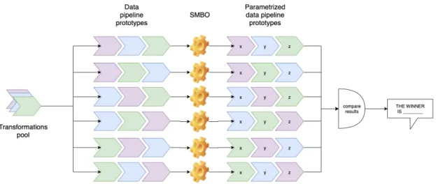
4.3 Online phase . . . 93 4.3.1 Data pipeline prototypes building . . . 93 4.3.2 Data pipeline prototypes optimization . . . 96
5 Evaluation 97
5.1 Data Pre-processing importance . . . 98 5.2 Evaluation of the Automated Data Pre-processing approach . . . 100
6 Conclusions and future developments 107
Listing of figures
2.1 Machine Learning process scheme . . . 18
2.2 Graphic representation of the outcome of a classifier . . . 21
2.3 Graphic representation of the cross validation technique . . . 24
2.4 Decision Tree example . . . 34
2.5 Example of how Decision Tree splits work . . . 35
2.6 Two-dimensional representation of K-Nearest Neighbor . . . 36
2.7 Trend of the growth of human and machine-generated data . . . 39
2.8 MLBase infrastructure . . . 43
2.9 Auto-Sklearn infrastructure . . . 47
2.10 Auto-Sklearn Pre-processing operators and machine learning algorithms 48 2.11 A Quemy’s pipeline instance . . . 49
2.12 Quemy’s reseacrh space . . . 49
3.1 SMBO algorithm example . . . 53
3.2 Gaussian Processes (GP) interpolation . . . 55
3.3 Example of a Regression Decision Tree . . . 57
3.4 Example of Random Forest . . . 57
3.5 Machine Learning problems scheme . . . 59
3.6 A combined hierarchical hyper-parameter optimization problem example 61 3.7 Hierarchical Dependencies in CASH and DPSO problems . . . 63
3.8 Quemy’s experiments results, accuracy changes in 100 iterations . . . . 64
3.9 Quemy’s experiments results, best pipelines explored . . . 65
4.1 Case in which the global application of the transformations is incorrect . 69 4.2 Previous case applying the transformations only to compatible attributes 69 4.3 Domain and Co-domain of the considered transformations . . . 70
4.4 Naive approach to consider all the data pipeline prototypes . . . 71
4.5 Online phase of our approach . . . 72
4.7 Offline phase that allows us to build the Dependency table . . . 74
4.8 Table resulting from the compatibility analysis . . . 75
4.9 Compatibility analysis, Encode-Normalize representation . . . 76
4.10 Compatibility analysis, Discretize-Normalize representation . . . 76
4.11 Table of constraints not considering the used framework . . . 77
4.12 Intermediate table construction . . . 78
4.13 Graphical representation of the performed SMBO experiments . . . 80
4.14 Result label extraction from the winning data pipeline . . . 81
4.15 Enumeration of all possible pipelines . . . 82
4.16 Graphs depicting the number of valid and invalid results . . . 83
4.17 Graphs depicting the labels about the valid results . . . 84
4.18 Graphs depicting the labels about the valid results . . . 84
4.19 Meta-learning working . . . 86
4.20 Graphs depicting the labels before and after the grouping . . . 87
4.21 Effects of Rebalancing step . . . 90
4.22 Example of assigning an order to the no_order instances . . . 91
4.23 Comparison of how to order no_order instances . . . 91
4.24 Study of meta-learners with different seeds . . . 92
4.25 Comparison of performances between GBM and XGBoost . . . 93
4.26 Table of constraints after the SMBO experiments . . . 94
4.27 BPMN scheme representing the possible data pipeline prototypes . . . . 95
5.1 Comparison between Pre-processing and Modeling optimizations . . . . 99
5.2 Comparison between our approach and the Quemy’s one . . . 101
5.3 Estimation of how much the winning approach improves the result . . . 103
5.4 Discretization transformation’s role in our pipeline . . . 104
List of Tables
2.1 Confusion Matrix . . . 21 3.1 A combined hierarchical hyper-parameter optimization problem example 62 4.1 Rules for validating and assigning the result label to two configurations . 82 4.2 Feature - Rebalance results . . . 89 4.3 Feature - Rebalance results with oversampling . . . 89 5.1 Comparison between Pre-processing and Modeling optimizations results 991
Introduction
Coca-Cola[25], with more than 500 drink brands sold in more than 200 countries, is the largest beverage company in the world. A monitoring system throughout all the supply chain generates a large amount of data and the company exploits it by supporting new product de-velopment.Heineken[26], a worldwide brewing leader, is looking to catapult its success in the United States by leveraging the vast amount of data they collect. From data-driven marketing[29], to the Internet of Things[24], to improving operations through data analytics[17], Heineken looks to improve its operations, marketing, advertising and customer service.
As we can see, the concept of Machine Learning[10]is growing in popularity, specially in the world of e-commerce and business activity. In Computer Science, Machine Learning is a field of study that gives computers the ability to learn without being explicitly programmed. In a nutshell, it means to acquire the capacity to observe, see patterns such as grouping of similar objects and then apply what it has been discovered. This is typically a human skill but
machines are even better in it because they can use more data and data with more dimensions. Most of the methods used in Machine Learning are exploited in Data Science[9] to analyze and extract information from the data. Vice versa, some Data Science techniques are fre-quently applied to improve Machine Learning results. In particular, in this thesis we analyze in detail the Pre-processing[20]techniques. Data Scientists transform the data through these techniques based on the nature of the data and the Machine Learning algorithm to be used. The Pre-processing step has become really important in the process of extracting knowledge from data, because nowadays more and more raw data perform poorly or cannot be directly consumed by Machine Learning algorithms as they are. All this comes from an exponential growth of Internet of Things, Web of Things[15], and Pervasive Computing[33]systems that produce large amounts of data, often unstructured, or otherwise not suitable for the algo-rithms in question. This growth has also led to an increase in the need to analyze such data and derive profit from it. The Data Scientist has become one of the most sought figures of the twenty-first century, but the numerous skills expected (IT, mathematics, statistics, business, cooperation) make it difficult to increase the number of Data Scientists. All this leads to non-expert users performing data analysis and Machine Learning without having the adequate knowledge. The result is that non-experts are overwhelmed by the large amount of available and applicable techniques, hence automatic tools that help them throughout the Machine Learning process are required. These tools are typically referred to as AutoML tools. Yet, they focus more on the application of Machine Learning algorithms and pay little attention to the Pre-processing part. Moreover, the few ones that actually support the automation of this phase provide just the application of a fixed series of transformations, called pipelines[32]. A fixed pipeline means that it is decided a priori, and it does not consider the nature of the data, the used algorithm, or simply that the order of transformations could affect the final result. The fixed pipeline approach is widely used, since trying out several different Pre-processing pipelines on a data-set is a highly expensive operation and the number of possible pipelines increases with the increase of the number of transformations involved.
In this thesis, we propose a new methodology that allows to recommend a Pre-processing pipeline according to the specific presented case. We studied the transformations, trying to understand their domain, co-domain and how they work. Thanks to this study we re-alized that, in some cases the semantics of transformations imposes a predetermined order.
In other cases, instead, it is the used technology that does not allow some pipelines. In this way we managed to decrease the total search space and therefore the number of pipelines to be tested. Moreover, since some constraints are not imposed neither by the semantics of the transformations nor by the used technology, but rather by the nature of the data-set and by the used algorithm, we had to perform some experiments. Specifically, we collected several different data-sets and, considering the most used Machine Learning algorithms, we tested various Pre-processing pipelines. In this way, we discovered hidden insights that the seman-tics of transformations did not show. But above all, we collected enough data to be able to use the Machine Learning algorithms themselves to discover the dependencies between transfor-mations, data-sets, and used algorithms. We were able to discard some other pipelines, and hence test just the promising ones. In order to evaluate the pipelines and choose the best one, we used the Bayesian techniques[3], which is state-of-the-art in this regard. Our approach takes into account the nature of the data, the algorithm we intend to use, and the impact that the order of transformations could have. This will open the road to more effective AutoML tools.
In chapter 2, we give a comprehensive introduction to Machine Learning, Data Science, and the application of these branches to real-case problems. In addition, we offer an analysis of the state-of-the-art of the available AutoML tools, with related pros and cons. In chapter 3, we provide a detailed explanation about Bayesian techniques and how they are applied in the AutoML field. Indeed, they underlie most AutoML tools, including ours. In chapter 4, we illustrate our approach and in 5, we discuss the results of some experiments performed with the aim to evaluate it. Finally, in 6, we discuss the contribution given by our research, the limitations of this work and outline future work.
2
Towards AutoML
In order to have a clear comprehension of the thesis, in this chapter it is given an introduction to the topic. Before talking about AutoML, which stands for Automated Machine Learning, a background of Machine Learning is needed and, no less important is its link with the Data Science field. In fact, the value of the entire project resolves around this connection.Once this knowledge is provided, we expose the objectives of the AutoML but also the need and the causes that led to the development of this branch. Further, we present a state-of-the-art overview and the related works on this topic.
2.1 Machine Learning
We use machines to solve problems, thus we write down a sequence of instructions and com-pose an algorithm, which in turn is capable of transforming an input to an output. Although this approach allows us to to solve a lot of problems, some others are not easily solved with an algorithm. For example, we can devise an algorithm to sort an array but not to distinguish spam and legitimate emails. We know the input and the output, respectively an email doc-ument and an answer yes/no indicating whether the message is spam or not, but we do not how to transform the input to the output.
We know that humans learn from their past experiences and machines follow instructions given by humans. But what if humans can train the machines to learn from past data? In other words, we would like to collect a set of messages, which we know if they are spam or not, and we would like the computer to learn how to distinguish them when a new email arrives.
In Figure 2.1 we can see a scheme that describes well the above mentioned example. The collected set of messages, from which the machine will learn to tell spam email from legitimate ones, is also called Train Set, sometimes abbreviated to TS. This name is coming from the fact that the computer is using it to train itself to understand the class (or label) of messages. In this case, the class is one of “spam” / “not spam”. The Machine Learning Algorithm is the core of the process, indeed, applying it the machine can learn. This phase is called Training or Learning Phase. The result is Model, the outcome of an induction process on the training set data. Through this a new message can be categorized: a prediction of the class can be inferred. Machine learning (ML) tasks are typically classified into three broad categories, depending on the nature of the learning method:
• Supervised learning, examples of inputs and related desired outputs are presented, thus the goal is to learn a general rule that maps inputs to outputs;
• Unsupervised learning, no desired output is given and the goal is to find a structure in the input;
• Reinforcement learning, the idea here is to learn through a dynamic environment. Some actions are performed and we want to understand which ones have a positive effect and which not. To achieve this goal, in addition to past data, the environment tells us, through a score, how well we are doing.
Another categorization of Machine Learning tasks arises when one considers, instead, the kind of input and output:
• Classification task, inputs are divided into two or more classes, and the learner must produce a model that assigns unseen inputs to one or (multi-label classification) more of these classes. This is typically tackled in a supervised way;
• Regression task, also a supervised problem, the outputs are continuous rather than discrete. For instance, predict the price of a used car given some car attributes that could affect a car’s worth, such as brand, year, mileage, etc.;
• Clustering task, a set of inputs has to be divided into groups. Unlike in classification, the groups are not known beforehand, making this typically an unsupervised task;
• Density estimation, the goal is to find the distribution of inputs in some space;
• Dimensionality reduction, simplifies inputs by mapping them into a lower-dimensional space.
Machine Learning covers a wide range of problems and, in order to fully understand them, each one requires its own in-depth study on the subject.
In this thesis, we focus on Supervised learning, in particular Classification problems. An example would be the problem of distinguishing between “spam” and “non spam” emails. First of all, we list the three different Classification types:
• Binary, assign an instance to one of two possible classes (often called positive and neg-ative one),
• Multiclass, assign an instance to one of n > 2 possible classes;
• Multilabel, assign an instance to a subset m ≤ n of the possible classes. Regardless of the number of the classes, the problem can be formalized as follows:
• The Machine Learning algorithm is provided with a set of input/output pairs (xi,yi) ∈
X × Y,
• The learned model consists of a function f : X −→ Y which maps inputs into their outputs (e.g. classify emails).
Training a model implies searching through the space of possible models (aka hypotheses). Such a search, typically aims at fitting the available training examples well according to a cho-sen performance measure. There are several measures with different meanings, and they are explained below.
Considering a Binary Classification problem, we have instances belonging to the positive class, for example “spam”, and others to the negative class, “not spam”. Usually the positive class is the one we are looking for, the one we are interested in distinguishing. Given the N instances to be classified, the result of each of the classification attempts can be:
• True Negative (TN): a negative instance has been correctly assigned to negatives; • False Positive (FP): a negative instance has been incorrectly assigned to positives. Also
called Type I or False error;
• False Negative (FN): a positive instance has been incorrectly assigned to negatives. Also called Type II or Miss error.
In Figure 2.2 we have a graphic representation.
Figure 2.2:Graphic representa on of the outcome of a classifier. FromWikimedia Commons, the free media repository.
The Confusion Matrix (Table 2.1) evaluates the ability of a classifier based on these indicators.
Predicted Class
Actual Class Positive Negative
Positive TP FN
Negative FP TN
In the cells TP, TN, FP and FN there are the absolute frequencies of the relative classifications and we can define the following metrics:
Accuracy : TP + TN
TP + TN + FP + FN = TP + TNN Misclassificationerror : FP + FN
TP + TN + FP + FN = 1 − Accuracy
Accuracy is the most widely used metric to synthesize the information of a Confusion Ma-trix but is not appropriate if the classes differ a lot in terms of the number of instances they contain. Considering a Binary Classification problem in which we have
• 9990 records of the first class; • 10 records of the second class;
A model that always returns the first class will have an accuracy of100009990 = 99.9%. A data-set like this one is called imbalanced data-set.
Precision and Recall are two metrics used in applications where the correct classification of positive class records is more important. Considering the positive class the “rare” one, we can have a clearer idea of the classifier’s behavior on these instances:
• Precision measures the fraction of record results actually positive among all those who were classified as such. High values indicate that few negative class records were incor-rectly classified as positive;
• Recall measures the fraction of positive records correctly classified. High values indi-cate that few records of the positive class were incorrectly classified as negatives; • F-measure is defined as the harmonic mean of Precision and Recall and, indeed,
Precision : TP TP + FP Recall : TP
TP + FN
F − measure : 2 ∗ Precision ∗ Recall Precision + Recall
Precision, Recall and F-measure are metrics that can be calculated for each class by reversing the positive class with the negative and vice versa.
In the case we have more than one class, the confusion matrix will be n×n, therefore a column and a row for each class, and the above metrics can be calculated for each class considering the class in question as positive and all the others as negative.
Last but not least, a metric similar to the Accuracy, but which avoids inflated performance estimates on imbalanced data-sets, is Balanced Accuracy[4,18]. It is the average of recall scores per class or, equivalently, raw Accuracy where each instance is weighted according to the in-verse prevalence of its true class. Thus for balanced data-sets, that metric is equal to Accuracy. Now that we know what performance measures are, we are going to understand how they can be used properly. In fact, if we measured the performance on the data used for training, we would overestimate its goodness.
It was already mentioned that training a model aims at learning a function which maps inputs into outputs. Even if this process is done through the instances at our disposal, the learned model should perform well on unseen data. Ideally, in a Machine Learning problem we have enough amount of data to both build the model and test it. Test the model means check effec-tively that it generalizes, that is, it also performs well on non-train data. This means evaluating the above metrics on the new instances. The way this is done is to split the whole amount of data into two portions: Train and Test Set. The algorithm is trained in the Train Set and tested in the Test Set. This method is called Hold-Out and generally it could be applied by keeping 60% (or 80%) of the data for the train and the remaining 40% (or 20%) for the test. However, in practice it happens that the only data available is that of the Training Set, or better said, it may happen that the data available is not enough for training and testing the model. This is where sampling techniques come into play to evaluate the model, without incurring Over-fitting or Under-fitting. Indeed the risk would be that of keeping the
Train-ing set big and the Test set small which leads to better accuracy in the learnTrain-ing phase. The model perfectly fits the data but it does not “learn the rule” and thus it does not generalize. The latter means that the model does not perform well on unseen data (Over-fitting). On the other hand, if the data for training is reduced, the algorithm may not have enough instances to build a good model and thus not capture enough patterns. This means it would perform poorly both in Train and Test Set (Under-fitting). Therefore, what is required is a method that provides sample data for training the model and also leaves sample data to validate it. K-Fold cross validation does exactly that. It can be viewed as repeated Hold-Out and we simply average scores after K different runs. In practice, the data set is divided into groups (folds) of equal number, iteratively excludes one group at a time and tries to predict it with the groups not excluded. Every data point gets to be in the Test Set exactly once, and gets to be in the Train Set k-1 times. This significantly reduces Under-fitting as we are using most of the data for fitting, and also significantly reduces Over-fitting as most of the data is also being used in Test Set. In Figure 2.3 we can observe a working example.
Figure 2.3:Graphic representa on of the cross valida on technique. From Georgios Drakos’s ar cle in Medium, Cross-Valida on[11].
This method is a good choice when we have a minimum amount of data and we get suffi-ciently big difference in result quality between folds. Through the number of folds we can control the used amount of data to train and test the learners in the folds. As a general rule, we
choose k=5 or k=10, as these values have been shown empirically to yield test error estimates that suffer neither from excessively high Bias nor high Variance.
• The Bias error is an error from erroneous assumptions in the learning algorithm. High Bias can cause an algorithm to miss the relevant relations between features and target outputs (Under-fitting);
• The Variance is an error from sensitivity to small fluctuations in the training set. High variance can cause an algorithm to model the random noise in the training data, rather than the intended outputs (Over-fitting).
Leave-one-out cross validation is K-fold Cross Validation taken to its logical extreme, with K equal to N, the number of instances in the set. That means that N separate times, the function approximator is trained on all the data except for one instance and a prediction is made for that instance. As before the average error is computed and used to evaluate the model. The evaluation given by Leave-One-Out Cross Validation is recommended in cases where the data-set is particularly small and you want to “lose” the least possible number of instances for the training but, in the meanwhile, we want to validate all the instances. A drawback of this approach is the cost involved for building as many models as the number of instances. A crucial point of the Cross Validation techniques is that their purpose is not to come up with our final model: assuming to use 5 folds, we do not use these 5 models to do any real prediction, for that we want to use all the data because we have to come up with the best model possible.
2.2 The Machine Learning role in Data Science
Nowadays several different companies are using Machine Learning techniques behind the scenes both to impact our everyday lives and to improve their own businesses. Specifically, a massive quantity of data is collected to make predictions and hence to take decisions that are more profitable for the company. The application of Machine Learning methods to large databases, with the purpose of extracting knowledge and useful information, is called Data Mining. The analogy is that a large volume of earth and raw material is extracted from a mine, which when processed leads to a small amount of very precious material; similarly, in Data
Mining, a large volume of raw data is processed to construct a simple model with valuable use. However, Data Mining is just a piece of a larger process called Knowledge Discovery in Databases, also abbreviated to KDD. The goal of knowledge discovery is wider than just applying Ma-chine Learning techniques and finding a suitable model. We are interested on what the data itself could bring, for example to detect similarities and to find interesting and unexpected patterns. Most of the time, we want to describe better the data, to reason about the infor-mation we find, and to understand and explain why there are certain patterns. Discovering knowledge from data should therefore be seen as a process containing several steps:
1. Domain & Data understanding;
2. Data Preparation, also called Pre-processing; 3. Data mining to discover patterns;
4. Post-processing of discovered patterns;
5. Results manipulations and interpretation, it is important to explain, read and present the results obtained in the correct way.
Below we will go deeper on the first three phases of this process, since they are those on which this thesis focuses.
2.2.1 Domain & Data understanding
Certainly a fundamental requirement for carrying out a useful analysis is having understood the domain of the data. Without that the Data Scientist, therefore the expert in charge to discover and reason about data, would not be able to take conscious decisions in the mining process. He has to know what the input means, how to interpret the results; he has to be able to recognize if a valuable outcome appears and, if not, why.
On the other hand, what makes a Data Science task different from a common Machine Learn-ing one is not the domain knowledge to acquire but rather that of data. KnowLearn-ing the nature of the data allows the Data Scientist to manipulate and transform it coherently. Usually in Machine Learning problems we have just numerical data, of the set of real numbers. In our
case the data-sets are more heterogeneous.
First of all, since we defined what a Classification task consist of, but we did not have formally defined what a data-set is, we proceed to explain it.
We said:
• The Machine Learning algorithm is provided with a set of input/output pairs (xi,yi) ∈
X × Y.
The set of all the (xi,yi) pairs provided as input constitutes the data-set. Specifically, each pair
is considered an instance, or record, and while yiis the class, therefore a single value belonging
to a finite set, xiis a more complex component. Indeed this latter is formed by columns,
commonly called features or attributes. These columns represent the characteristics of each instance; in other words they provide a description of it. Previously we also said:
• The learned model consists of a function f : X −→ Y which maps inputs into their outputs (e.g. classify emails).
Even here, considering what we have just explained, we can go deeper in what the model con-sists of. Think, for example, of a supermarket chain that has hundreds of stores all over a country, selling thousands of goods to millions of customers. The point of sale terminals record the details of each transaction: date, customer identification code, goods bought and their amount, total money spent, and so forth. We now know that these represent the fea-tures. What the supermarket chain wants, is to be able to predict who are the likely customers for a product. Considering the product’s type as class, the Machine Learning algorithm is try-ing to find some patterns in the features that allow the supermarket to determine the prod-uct’s type. So, the learned model f : X −→ Y establishes relations between the domain of the features and the domain of the classes.
Features can be of the following types:
• Numerical, express a measurable quantity and they could be of two kinds:
– The ones where the difference between the values has a meaning, i.e. there is a
– The ones which also have an absolute zero and hence the ratio between the values
has a meaning too, e.g. age, mass, length and so on;
• Categorical, they express qualitative phenomena and stand out in:
– Nominals, different names of values. We can only distinguish them, e.g. gender
or eyes color;
– Ordinals, values which allow us to sort objects based on the attribute value such
as a rating or the hardness of a mineral.
There are actually many other types of data, such as images, text, space-time data and so on. Generally the area of data mining focuses on categorical and numerical data, also called struc-tured data. Another type that we could run into in this category is the Timestamp, sequence of characters or encoded information identifying when a certain event occurred, usually giv-ing date and time of day, sometimes accurate to a small fraction of a second.
2.2.2 Data Preparation
As we just said in the previous section, knowing the nature of the data allows the Data Scien-tist to manipulate and transform it coherently. The transformations which he uses are called Pre-processing transformations because they are applied before the Machine Learning pro-cess. It has been proven that they improve the classifier to predict better[2]. In litterature , there are several different transformations:
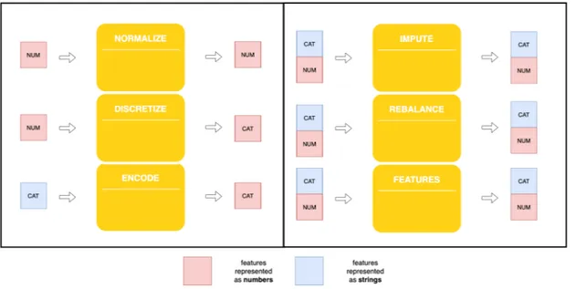
• Imputation; • Rebalancing; • Features Engineering; • Discretization; • Normalization; • Encoding.
For each one we have many available operators; in this section we will go into detail on each of them.
We start talking about the Imputation techniques. Sometimes, for some instances, the value of some attributes could not be present. This could happen because the information was not collected, e.g. the interviewee did not indicate his age and weight, or the attribute is not applicable to all objects, e.g. the annual income does not make sense for children. However, there are several different ways to handle it:
• Delete the objects that contain them, if the data-set is sufficiently numerous; • Let the algorithm handle them;
• Manually fill in the missing values, generally too time consuming;
• Automatically fill in missing values, using the so called Imputation techniques. These techniques are divided into:
• Univariate imputation techniques, which enter a constant value in place of missing values or estimate them with the mean (or the mode) of the attribute in question; • Multivariate imputation techniques, for each instance predict the value of the missing
attribute based on other known attributes. In this case, Data Mining algorithms would be used to prepare input data for other Data Mining algorithms.
Instead, regarding the Re-balancing techniques, we are using them when we have to deal with data-sets in which one or more classes have a far greater, or lesser, number of instances than the others. These kinds of data-sets are called imbalanced data-sets and, using the data as it is, could create problems when Machine Learning algorithms are applied. Since the goal of the algorithms is to maximize the predictive accuracy, that is equivalent to minimize the mis-classification error, for the classifier is more convenient to have a prediction tending towards the majority class. In that way we would have a model which will not generalize. The Re-balancing, also called re-sampling techniques were conceived to equilibrate the number of instances for each class, making the algorithm learn on a balanced training data-set.
• Under-sampling, involves dropping some instances from the majority classes; • Over-sampling, involves supplementing the instances of the minority classes.
Both have several different techniques, most of them based on the K-Nearest Neighbor Ma-chine Learning algorithm. In a nutshell, the points of the training set are drawn in a multi-dimensional space and, instead of discarding/adding points randomly, the sampling is done in such a way as to maintain consistency with existing points. For the Under-sampling family we can mention the NearMiss[37]and CondensedNearestNeighbor[16]techniques which try to keep the distribution as representative as possible. For the Over-sampling family we can mention the SMOTE[6]technique which on the other hand generates synthetic data points based on the distance between the points in the multi-dimensional representation.
The Feature Engineering techniques are used because, as the dimensionality increases (num-ber of features in the data-set), the data becomes progressively more scattered and many Clus-tering and Classification algorithms have difficulties when dealing with data-sets that have high dimensions. The definitions of density and distance between points becomes less sig-nificant, fundamental in algorithms such as the aforementioned K-Nearest Neighbor. This phenomenon is called Curse of Dimensionality and the Features Engineering techniques are used to deal with it:
• Principal Component Analysis (PCA), it is a projection method that transforms ob-jects belonging to a p-dimensional space into a k-dimensional space (with k < p) pre-serving the maximum information in the initial dimensions (the information is mea-sured as total variance of the data-set);
• Feature selection, it aims at completely discarding some features from the analysis. In particular, it is performed because some of them could be:
– Redundant, therefore duplicate the information contained in other attributes
due to a strong correlation between information;
– Irrelevant, for instance the student’s ID is often useless to predict the average of
the grades.
– Exhaustive approach, test all possible subsets of attributes and choose the one
that provides the best results on the test set using the predicted accuracy of the mining algorithm as goodness function. Given n attributes, the number of pos-sible subsets is 2n− 1;
– Non-exhaustive approaches:
*
Embedded approaches, the selection of attributes is an integral part of the Data Mining algorithm. The algorithm itself decides which attributes to use (e.g. Decision Trees);*
Filtered approaches, the selection phase takes place before mining and with criteria independent of the algorithm used (e.g. sets of attributes are chosen whose element pairs have the lowest correlation level);*
Heuristic approaches, approximate the exhaustive approach using heuristic search techniques.Discretization means transformation of numerical attributes into categorical attributes, ag-gregating values in intervals or categories. Indispensable to use some mining techniques (e.g. Association Rules) and it can also be used to reduce the number of categories of a discrete attribute.
Discretization requires to:
• Find the most suitable number of intervals; • Define how to choose split points.
And there are two kinds of techniques:
• Unsupervised, do not exploit the knowledge about the class to which the elements belong;
• Supervised, exploit the knowledge on the class to which the elements belong. For the unsupervised family we can list the following techniques:
• Equi-Frequency, also called Equi-Height, the range is divided into intervals with the same, or similar, number of elements;
• K-medians, k groupings are identified in order to minimize the distance between the points belonging to the same grouping.
Regarding the supervised discretization, the intervals are positioned in order to maximize their “purity”. We fall into a classification problem: starting from classes, the intervals com-posed of a single element, contiguous classes are merged recursively. A statistical measure of purity is the entropy of the intervals. Each value v of an attribute A is a possible boundary for division into the intervals A ≤ v ∧ A > v. We choose the value which preserves the greatest information gain, i.e. the greatest reduction in entropy. The process is applied recursively to the sub-intervals thus obtained, until a stop condition is reached, for example until the information gain obtained becomes less than a certain threshold d.
Normalization techniques involve the application of a function that maps the entire set of val-ues of an attribute into a new set so that each value in the starting set corresponds to a single value in the arrival set. This allows the entire set of values to respect a certain property and this is necessary to compare variables with different variation intervals. For example, think of having to compare a person’s age with his income. In a classification problem, where you want to predict the job of a person, an income difference of 50€ between two people means they are similar, instead, 50 years of difference lead you to consider a completely different class. We mention the two main Normalization techniques:
• Max-Min normalization, the A attribute is rescaled so that the new values fall between a new range: NewMinA and NewMaxA. The new value x′is calculated from the start-ing value x as follow:
x′= x − MinA
MaxA− MinA ∗ (NewMaxA − NewMinA) + NewMinA
• Z-score normalization, it changes the distribution of the A attribute so that it has mean 0 and standard deviation 1:
x′= x − μA
μAis the mean of the A attribute and δAits standard deviation.
In conclusion, there are the Encoding techinques. Often some algorithm implementations are not working with categorical features. This causes an incompatibility between the data we have and the data accepted. We have to convert the categorical features into numerical: encode. There are mainly two techniques types:
• Ordinal Encoding, it transforms each categorical feature to one new feature of integers (0 to n_categories - 1);
• One-Hot Encoding, it transforms each categorical feature with n_categories possible values into n_categories binary features, with just one of them 1, and all others 0.
2.2.3 Data mining
Many learning techniques seek structural descriptions of what is learned, descriptions that can become quite complex as sets of rules or decision trees. Since these descriptions can be understood by people, they serve to explain what has been learned; in other words, to explain the basis for new predictions. There are also other techniques, such as the Artificial Neu-ral Networks (ANN), called black box techniques, which geneNeu-rally perform very well but are effectively incomprehensible. Experience shows that, in many applications of Machine Learning to Data Mining, the explicit knowledge structures acquired and the structural de-scriptions are, at least, as important as the ability to obtain good results on new examples. People often use data mining to gain knowledge, not just predictions. Getting knowledge from the data is certainly something that enriches the result.
Below we illustrate three of the most used algorithms in the field of Data Mining. In particu-lar, since there are many peculiarities for each one, we will only argue the basic idea on which they are based. We will explain the functioning of these particular algorithms, and not others, both for the high expressiveness of some of them and also because they have been used in this thesis project.
Decision Trees are one of the most widely used classification techniques that allow to repre-sent a set of classification rules with a tree. A tree is a hierarchical structure consisting of a set of nodes, linked by labeled and oriented arcs. There are two types of nodes:
• Leaf nodes which identify classes;
• The others which are labeled based on the attribute that partitions the instances. The partitioning criterion represents the label of the arcs and each root-leaf path represents a classification rule.
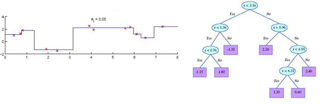
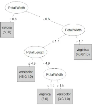
Figure 2.4:Decision Tree example on the Iris data-set, built using the well-known machine learning framework Weka.
In Figure 2.4 we see an example of a Decision Tree built on the Iris data-set. Iris is a genus of plants that contains over 300 species. In the data-set in question there are 154 instances of Iris classified according to three species: Iris setosa, Iris virginica and Iris versicolor. The four features considered are the length and width of the sepal and petal. We can notice that in the tree’s leafs some numbers are reported. It is not a coincidence that the sum of these is the size of the data-set, indeed they represent the number of instances of the training set classified according to the leaf. When only one number is present in the leaf node, it means that all the instances in question have been correctly classified. Instead, in the case that two
numbers are present, the first number represents the instances correctly classified, the second number counts the elements classified as such but belonging to another class.
Figure 2.5:Example of how Decision Tree splits work.
Decision tree expressivity is limited to the possibility of performing search space partitions with conditions that involve only one attribute at a time: the decision boundary are parallel to the axes. In Figure 2.5 we have an example. On the other hand, Decision trees are robust to strongly correlated attributes because, in each split, they automatically assesses which at-tributes to divide; and if there is a correlation between two atat-tributes, one of them will not be considered. A complex issue to address is to find the optimal split point in each attribute but a Discretization technique can be used to manage the complexity of the search.
K-Nearest Neighbor is an algorithm that, unlike the others, does not build models but classify the new records based on their similarity to the instances in the Train Set, for this reason they are called lazy learners. We can say that, in a certain way, the Train Set is the model itself. When a new instance needs to be classified, the nearest k points (neighbors) are used to per-form the classification. The basic idea is: “if it walks like a duck, quacks like a duck, then it’s probably a duck”.
Figure 2.6:Two-dimensional representa on of K-Nearest Neighbor.
They require:
• The training set;
• A metric to calculate the distance between records; • The value of k, which is the number of neighbors to use. The classification process involves:
• To calculate the distance to the instances in the training set • To identify the k nearest neighbors
• To use the classes of the nearest neighbors to determine the class of the unknown in-stance (e.g. choosing the one that appears most frequently)
The classification of a new instance z is obtained through the majority voting process among Dz, therefore the k closest elements of the training set D:
yz = argmaxy∈Y
∑ (xi,yi)∈Dz
where Y is the set of class labels and and function I returns 1 if its argument is TRUE, 0 otherwise.
To operate correctly, the attributes must have the same scale of values and must therefore be normalized during the Pre-processing phase. For example a difference of 0.5 is more signif-icant on an attribute in which the range varies from 1.5 to 2.5 rather than on an attribute that varies from 50 to 150. Moreover, they are very sensitive to the presence of irrelevant or related attributes that will distort the distances between objects. For example if in a data set of commercial products, in addition to standard attributes such as product category, year of production and so on, we have the attributes “price without taxes” and “price with taxes”, as high values of one correspond to high values of the other, the price will have more importance than normal. A Pre-processing step, such as feature selection or PCA, solves the problem. Naive Bayes classifiers represent a probabilistic approach by modeling probabilistic relation-ships between attributes and the class.
The conditional probability P(A|C) is the probability that the event A occurs knowing that the event C has occurred. P(A,C) is the joint probability of the two events A and C, there-fore the probability that both occur and it is defined as the conditional probability P(A|C), multiplied by the probability that C actually occurs:
P(A,C) = P(A|C)P(C) = P(C|A)P(A) Consequently we can define:
P(C|A) = P(A,C)P(A) P(A|C) = P(A,C) P(C)
and with a simple mathematical equation we can reach the Bayes theorem:
P(C|A) = P(A,C)P(A) = P(A|C)P(C)P(A) P(A|C) = P(A,C)P(C) = P(C|A)P(A)P(C)
Let the vector A = (A1,A2, ...,An) describe the set of attributes and let C be the class variable.
If C is linked in a non-deterministic way to the values assumed by A we can treat the two variables as random variables and capture their probabilistic relationships using P(C|A):
• Before the training phase, the probabilities P(C) and P(A) are calculated through the training set;
• During the training phase, the probabilities P(C|A), called also a priori probabilities, are learned for each combination of values assumed by A and C;
• Knowing these probabilities and applying the Bayes theorem, for a test record with certain attributes values a, we calculate for each class c, the posterior probability P(c|a). Then, we classify the test instance with the class which maximizes that posterior prob-ability.
The main advantage of probabilistic reasoning over logical reasoning lies in the possibility of reaching rational descriptions even when there is not enough deterministic information on the functioning of the system. Since it is based on the calculation of the probabilities they are very robust to: irrelevant features and noise:
• The noise is canceled during the calculation of P(A|C);
• If A is an irrelevant attribute, P(A|C) is uniformly distributed with respectto the values of C and therefore its contribution is also irrelevant.
A drawback could be that related attributes can reduce effectiveness since the assumption of conditional independence does not apply to them. However, we already know that this problem can be resolved through feature selection or PCA techniques.
2.3 The AutoML approach
We are overwhelmed with data. The amount of data in the world, in our lives, seems ever-increasing and there is no end in sight. In fact, it has been reported that 2.5 quintillion bytes of data is being created everyday and the 90% of stored data in the world, has been generated in the past two years only[27]. Specifically, human and machine-generated data is experiencing an overall 10x faster growth rate than traditional business data, and machine data is increasing even more rapidly at 50x that growth rate. In Figure 2.7 the reported data from[28].
Figure 2.7:Trend of the growth of human and machine-generated data, from the ar cle IoT, Big Data and AI - the new
“superpowers” in the digital universe published in Forbes[28].
By business data we mean all the data generated in the traditional way so far by companies, such as interviews, questionnaires and market surveys. However over the years the advance-ment of technology has led to a change in the market. With human-generated data we means UGC, short for User-Generated Content, the term which describes any form of content such as video, blogs, discussion form posts, digital images, audio files, and other forms of media that is created by consumers or end-users of an online system or service. It is becoming an important part of content marketing, with consumers forming a part of a brand’s strategy. It is powerful because it builds connections between like-minded people, whether the oppor-tunity is to share a common experience or win a prize.
We instead refer to pervasive computing, or ubiquitous computing, the growing trend of embedding computational capability into everyday objects to make them effectively com-municate and perform useful tasks in a way that minimizes the end user’s need to interact with computers as computers. Pervasive computing devices are network-connected and con-stantly available. Such devices, equipped with sensors, measure a substantial amount of data, called machine-generated data.
It is precisely these phenomena, UGC and pervasive computing, that led to a dizzying in-crease in human and machine-generated data and led us to the era of data ubiquity: data is central to all of our existences, whether we’re a giant enterprise or an individual person. As a consequence of this unceasing growth of data, the need to organize and exploit the stored data has also increased dramatically. Above all this need is coming from companies, to make more conscientious business decisions. Essentially, it can be said that the Data Scientist is the expert that the companies are looking for, capable of extrapolating insights and analyzes. His figure must have heterogeneous skills, ranging from technology to knowledge of the mar-ket and business, up to the ability to use Machine Learning techniques and programming languages:
• Math & Statistic skills which comprises Machine Learning, Statistical Modeling, Data Science fundamentals, etc.;
• Programming & Database skills which comprises of Computer Science fundamentals, scripting and statistical languages, Databases, Big Data tools, etc.;
• Domain Knowledge & Soft skills which comprises of being passionate about the busi-ness, curios about data, strategic, proactive, creative and so on;
• Communication & Visualizazion skills which comprises of being able to translate data-driven insights into decisions and actions, know how to use visualization tools, be able to engage with senior management, etc.
However, although this exponential growth in data has led to the new business position of Data Scientist and with it to new opportunities, it has been reported that the demand is far greater than the supply. Data Scientists cannot scale: it is almost impossible to balance the
number of qualified experts of this field and the required effort to analyze the increasingly growing sizes of available data[14]. This gap has led to more and more non-expert users to approach this world and carry out data analysis, using Data Mining techniques. The pro-cess itself, known as Knowledge Discovery in Databases (KDD), consists of several steps, and users are overwhelmed by the amount of Machine Learning algorithms and Pre-processing techniques. These users require off-the-shelf solutions that will assist them throughout the whole process.
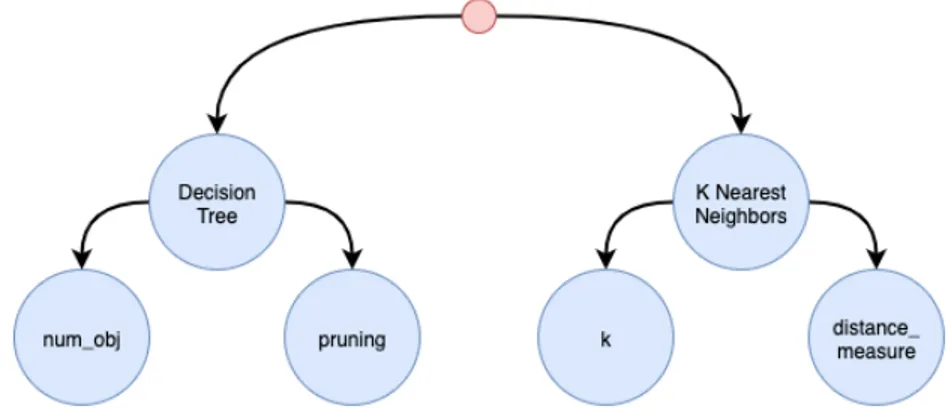
Indeed, the problems are related to these two main KDD phases. Regarding the Model-ing phase, the difficulty is buildModel-ing a high-quality Machine LearnModel-ing model; the process to achieve this result is iterative, complex and time-consuming. The Data Scientist needs to se-lect among a wide range of possible algorithms (e.g. Decision Trees, K-Nearest-Neighbor, Naive Bayes, etc.) and to tune numerous hyper-parameters of the selected algorithm. An al-gorithm hyper-parameter is a parameter that the Machine Learning alal-gorithm cannot learn by itself and, hence, it must be set a priori. For instance, common parameters in the Decision Tree are the attributes splits chosen by the algorithm; instead, a hyper-parameter would be the number of instances reacquired in a leaf to be split again. Regarding the Pre-processing step, the issue is to find the techniques to use. To automate this process we have to take in consideration more variables:
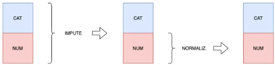
• There are several different transformations, e.g. Imputation, Re-balancing, Features Engineering, Discretization, Normalization, Encoding;
• For each transformation we have several operators, e.g. Normalization Min-Max, Nor-malization Z-score, etc.;
• For each operator we have different parameters; • The order in which they are applied affects the result.
Moreover, the problem is more complicated because the transformations application de-pends on both the chosen algorithm and the data-set itself. A sequence of Pre-processing transformations, with related operators and parameters, is called data pipeline. Instead a Ma-chine Learning pipeline (ML pipeline) consists of a data pipeline and a MaMa-chine Learning al-gorithm with its hyper-parameters defined. The techniqueof automatically configuring ML
pipelines is called AutoML.
Unfortunately, existing solutions either do not recommend Pre-processing operators or they recommend them in a very poor way, not giving too much importance to this step. In-deed, it has been noticed that the automation of the Modeling problem is performed in 16 out of 19 selected publications while only 2 publications study the automation of Data Pre-processing[7]. This fact represent an issue because generally raw data do not perform very well. Indeed, pervasive computing systems greatly increased the amount of machine-generated data and, since we are talking about data machine-generated by sensors, we are rarely having data ready to be consumed. All in all, the Pre-processing phase plays a key role in Machine Learning and it is require a tool which treats all the problems (Modeling and Pre-processing ones) in all its complexity.
2.4 The state-of-the-art solutions
In this section, we provide an overview of several tools and frameworks that have been imple-mented to automate Modeling and Pre-processing problems. In general, they can be classified into three main categories: distributed, cloud-based and centralized. In order to be able to work with large quantities of data, distributed and cloud-based distributions use clusters and therefore different techniques than centralized solutions. A cluster is a set of machines that work together so that, in many respects, they can be viewed as a single system. For data-sets with not exaggerated quantities of instances, the overhead of using the cluster is not worth-while and centralized solutions are preferred.
2.4.1 Distributed tools
MLbase[22,35]has been the first work to introduce the idea of developing a distributed envi-ronment for Machine Learning algorithm selection and hyper-parameter optimization. It is based on Apache Spark, an open source framework for distributed computing and a unified analytics engine for big data processing. In particular MLlib is the Spark library which al-lows to use the Machine Learning algorithm in distributed manner. MLBase exploit Spark’s functionalities and MLlib, it consists of three components (Figure 2.8):
• ML Optimizer, this layer aims to automating the task of ML pipeline construction. The optimizer solves a search problem over feature engineering and ML algorithms included in MLI and MLlib. The ML Optimizer is currently under active develop-ment;
• MLI[34], an experimental API for feature engineering and algorithm development that introduces high-level ML programming abstractions. A prototype of MLI has been implemented against Spark, and serves as a testbed for MLlib;
• Apache Spark’s distributed ML library. MLlib was initially developed as part of the MLbase project, and the library is currently supported by the Spark community. Many features in MLlib have been borrowed from ML Optimizer and MLI, e.g. the model and algorithm APIs, multimodel training, sparse data support, design of local / dis-tributed matrices, etc.
Figure 2.8:MLBase infrastructure. From theofficial MLBase documenta on.
TransmogrifAI[1]is a really recent tool written in Scala. Currently, TransmogrifAI supports eight different binary classifiers, five regression algorithms and it expects a minimal human involvement.
MLBox is a Python-based AutoML framework covering several processes, including Pre-processing, optimization and prediction. It supports model stacking where a new model is
trained from combined predictors of multiple previously trained models and it uses opt, a distributed asynchronous parameter optimization library to perform the hyper-parameter optimization process.
2.4.2 Cloud-based tools
Google Cloud AutoML is a suite of Machine Learning products that allows developers with limited experience in the field of Machine Learning to train high-quality models based on business needs. It is based on Google’s cutting-edge Transfer Learning (TL)[36]and Neural Architecture Search (NAS)[12]technologies. Transfer learning focuses on storing knowledge gained while solving one problem and applying it to a different but related problem. For example, knowledge gained while learning to recognize cars could apply when trying to rec-ognize trucks. Over the years, Google has memorized a lot of data about different problems which allows to have really valid recommendations. Instead, Neural Architecture Search is a technique for automating the design of Artificial Neural Networks.
Google Cloud AutoML build models in different domains and for various tasks:
• AutoML Vision and AutoML Video Intelligence allow respectively to get insights from image and perform content detection;
• AutoML Natural Language and AutoML Translation detect the structure and mean-ing of the text and translate dynamically from one language to another;
• AutoML Tables, automatically develops and deploys the latest generation machine learning models on structured data.
Focusing on AutoML Tables, it performs automatically both model building and some data Pre-processing. The data Pre-processing that AutoML Tables does includes:
• Normalization and discretization of numeric features; • Application of one-hot encoding for categorical features; • Performing basic processing for text features;
Moreover, missing values are handled according to the type of the features: • Numerical, a 0.0 or −1.0 is imputed;
• Categorical, an empty string is imputed; • Text, an empty string is imputed;
• Timestamp, a timestamp set to −1 is imputed.
Then, when the model training kicks off, AutoML Tables takes the data-set and starts train-ing for multiple model architectures at the same time. This approach enables AutoML Tables to determine quickly the best model architecture, without having to serially iterate over the many possible model architectures. AutoML Tables tests includes:
• Linear Regression, one of the most simple but effective regression algorithm;
• Feedforward Deep Neural Network, a kind of Artificial Neural Networks which in these last years allows to solve a wide range of problems;
• Gradient Boosted Decision Tree, classifier which combines several different Decision Trees in order to take the best of everyone;
• AdaNet, a particular algorithm which learn the structure of a neural network as an ensemble of subnetworks;
• Ensembles of various model architectures, like in Gradient Boosted Decision Tree and AdaNet, the goal is to define a combined learner that performs better than a basic one. Azure AutoML uses collaborative filtering to search for the most promising pipelines effi-ciently based on a database that is constructed by running millions of experiments of evalu-ation of different pipelines on many data-sets. With collaborative filter we refer to a class of tools and mechanisms that allow the retrieval of predictive information regarding the inter-ests of a given set of users. Collaborative filtering is widely used in recommendation systems, in this case what is recommended is the ML pipeline.
and Deep Learning frameworks to build their models in addition to automatic tuning for the model parameters. Moreover, Amazon offers a long list of pre-trained models for different AI services that can be easily integrated to user applications, such as image and video analysis, voice recognition, text analytics, forecasting and recommendation systems.
2.4.3 Centralized tools
Several tools have been implemented on top of widely used centralized machine learning packages which are designed to run in a single node (machine). In general, these tools are suitable for handling small and medium sized data-sets. Since the problem to address is a op-timization problem, find a maximum or minimum of a unknown function, various are the techniques used in this category. However we list only two because they are the most used:
• Genetic algorithms, which are inspired by the branch of genetics, and allow to evalu-ate different starting evaluations (as if they were different biological individuals) and, by recombining them (analogous to sexual biological reproduction) and introducing elements of disorder (analogous to random genetic mutations), they produce new so-lutions (new individuals) that are evaluated by choosing the best (environmental se-lection) in an attempt to converge towards “excellent” solutions.
• Bayesian optimization techniques, which are based on Bayes Theorem, start from a bunch of random evaluations and try to approximate the objective function through regression techniques and a probabilistic model. There are three different implemen-tation of it:
– Using Gaussian Procces (GP);
– Tree-structured Parzen Estimators (TPE);
– Sequential Model-based Algorithm Configuration (SMAC).
As this approach has captured more attention recently, a more comprehensive expla-nation will be provided in the next chapter.
Auto-Weka[21] is considered as the first and pioneer Machine Learning automation frame-work[21]. It has been implemented in Java on top of Weka, a popular Machine Learning
library that has a wide range of machine learning algorithms. Auto-Weka applies Bayesian op-timization using SMAC and TPE implementations for both algorithm selection and hyper-parameter optimization (Auto-Weka uses SMAC as its default optimization algorithm but the user can configure the tool to use TPE). No Pre-processing recommendation is done. Auto-Sklearn[13]has been implemented, instead, on top of the competitor framework Scikit-Learn, a Python package. Auto-Sklearn used SMAC as a Bayesian optimization technique too but in order to improve the quality of the result introduced a meta-learer. Indeed, the outcome of these techniques of optimization depends a lot on the start evaluations. The idea is to retrieve data-sets similar to the one in input and feed SMAC with the solutions of those similar data-sets. The component in charge of this task is called meta-learner since it is built through a Machine Learning algorithm and the similarity through data-sets is com-puted thanks to the meta-data (data that describes data). In addition, ensemble methods were also used to improve the performance of output models. With ensemble methods we refer to a set of techniques which aim to improve the quality of the result by combining the results of the best learner found. In Figure 2.9 we can see the infrastructure just described.
Figure 2.9:Auto-Sklearn infrastructure, from Efficient and Robust Automated Machine Learning published in NIPS 2015[13].
Unlike the previous tool, this one allows, although poor, some Pre-processing. The included transformations are as follows, in the following fixed order:
• Encoding (just one operator); • Imputation (just one operator); • Normalization (just one operator);
• Balancing (just one operator);
• Features Pre-processing (thirteen operators).
The Modeling step follows with a choice of fifteen algorithms. In Figure 2.10 the Pre-processing operators and Machine Learning algorithms used in[13]are listed.
Figure 2.10:Sklearn Pre-processing operators and machine learning algorithms, from Efficient and Robust
Auto-mated Machine Learning published in NIPS 2015[13].
The work of A. Quemy in[32] focuses on applying the Bayesian techniques just to the Pre-processing pipeline, ignoring the Modeling phase, but extending the research space of Data Preparation, increasing the number of operations of each transformation. Below an instance of the data pipeline (Figure 2.11) and the considered research space (Figure 2.12) is shown.
![Figure 2.9: Auto-Sklearn infrastructure, from Efficient and Robust Automated Machine Learning published in NIPS 2015 [ 13 ] .](https://thumb-eu.123doks.com/thumbv2/123dokorg/7385902.96855/47.918.219.640.591.656/figure-sklearn-infrastructure-efficient-automated-machine-learning-published.webp)
![Figure 2.12: Quemy’s research space, from Data Pipeline Selec on and Op misa on published in DOLAP 2019 [ 32 ] .](https://thumb-eu.123doks.com/thumbv2/123dokorg/7385902.96855/49.918.130.804.439.783/figure-quemy-research-space-pipeline-selec-published-dolap.webp)