arXiv:1302.4893v1 [astro-ph.SR] 20 Feb 2013
Atmosphere above a large solar pore
M Sobotka1, M ˇSvanda1
,2, J Jurˇc´ak1, P Heinzel1 and D Del Moro3
1
Astronomical Institute, Academy of Sciences of the Czech Republic (v.v.i.), Friˇcova 298, CZ-25165 Ondˇrejov, Czech Republic
2
Charles University in Prague, Faculty of Mathematics and Physics, Astronomical Institute,
V Holeˇsoviˇck´ach 2, CZ-18000 Prague 8, Czech Republic
3
Department of Physics, University of Roma Tor Vergata, Via della Ricerca Scientifica 1, I-00133 Roma, Italy
E-mail: [email protected]
Abstract. A large solar pore with a granular light bridge was observed on October 15, 2008
with the IBIS spectrometer at the Dunn Solar Telescope and a 69-min long time series of spectral scans in the lines Ca II 854.2 nm and Fe I 617.3 nm was obtained. The intensity and Doppler signals in the Ca II line were separated. This line samples the middle chromosphere in the core and the middle photosphere in the wings. Although no indication of a penumbra is seen in the photosphere, an extended filamentary structure, both in intensity and Doppler signals, is observed in the Ca II line core. An analysis of morphological and dynamical properties of the structure shows a close similarity to a superpenumbra of a sunspot with developed penumbra. A special attention is paid to the light bridge, which is the brightest feature in the pore seen in the Ca II line centre and shows an enhanced power of chromospheric oscillations at 3–5 mHz. Although the acoustic power flux in the light bridge is five times higher than in the ”quiet” chromosphere, it cannot explain the observed brightness.
1. Introduction
Pores are small sunspots without penumbra. The absence of a filamentary penumbra in the photosphere has been interpreted as the indication of a simple magnetic structure with mostly vertical field, e.g. [1, 2]. Magnetic field lines are observed to be nearly vertical in centres of pores and inclined by about 40◦ to 60◦ at their edges [3, 4]. Pores contain a large variety of fine bright features, such as umbral dots and light bridges that may be signs of a convective energy transportation mechanism.
Light bridges (hereafter LBs) are bright structures in sunspots and pores that separate umbral cores or are embedded in the umbra. Their structure depends on the inclination of local magnetic field and can be granular, filamentary, or a combination of both [5]. Many observations confirm that magnetic field in LBs is generally weaker and more inclined with respect to the local vertical. It was shown in [6] that the field strength increases and the inclination decreases with increasing height. This indicates the presence of a magnetic canopy above a deeply located field-free region that intrudes into the umbra and forms the LB. Above a LB, [7] found a persistent brightening in the TRACE 160 nm bandpass formed in the chromosphere. It was interpreted as a steady-state heating possibly due to constant small-scale reconnections in the inclined magnetic field.
In the chromosphere, large isolated sunspots are often surrounded by a pattern of dark, nearly radial fibrils. This pattern, called superpenumbra, is visually similar to the white-light penumbra
but extends to a much larger distance from the sunspot. Dark superpenumbral fibrils are the locations of the strongest inverse Evershed flow – an inflow and downflow in the chromosphere toward the sunspot. Time-averaged Doppler measurements indicate the maximum speed of this flow equal to 2–3 km s−1 near the outer penumbral border [8].
2. Observations and data processing
A large solar pore NOAA 11005 was observed with the Interferometric Bidimensional Spectrometer IBIS [9] attached to the Dunn Solar Telescope (DST) on 15 October 2008 from 16:34 to 17:43 UT, using the DST adaptive optics system. The slowly decaying pore was located at 25.2 N and 10.0 W (heliocentric angle θ = 23◦) during our observation. According to [10], the maximum photospheric field strength was 2000 G, the inclination of magnetic field at the edge of the pore was 40◦ and the whole field was inclined by 10◦ to the west.
The IBIS dataset consists of 80 sequences, each containing a full Stokes (I, Q, U, V ) 21-point spectral scan of the Fe I 617.33 nm line (see [10]) and a 21-point I-scan of the Ca II 854.2 nm line. The wavelength distance between the spectral points of the Ca II line is 6.0 pm and the time needed to scan the 0.126 nm wide central part of the line profile is 6.4 s. The exposure time for each image was set to 80 ms and each sequence took 52 seconds to complete, thus setting the time resolution. The pixel scale of these images was 0′′.167. Due to the spectropolarimetric setup of IBIS, the working field of view (FOV) was 228 × 428 pixels, i.e., 38′′× 71′′.5. The detailed description of the observations and calibration procedures can be found in [10,11].
Complementary observations were obtained with the HINODE/SOT Spectropolarimeter [12,13]. The satellite observed the pore on 15 October 2008 at 13:20 UT, i.e., about 3 hours before the start of our observations. From one spatial scan in the full-Stokes profiles of the lines Fe I 630.15 and 630.25 nm we used a part covering the pore umbra with a granular LB.
According to [14], the inner wings (±60 pm) of the infrared Ca II 854.2 nm line sample the middle photosphere at the typical height h ≃ 250 km above the τ500= 1 level, while the centre of this line is formed in the middle chromosphere at h ≃ 1200–1400 km. This provides a good tool to study the pore and its surroundings at different heights in the atmosphere and to look for relations between the photospheric and chromospheric structures.
The observations in the Ca II line are strongly influenced by oscillations and waves present in the chromosphere and upper photosphere. The observed intensity fluctuations in time are caused by real changes of intensity as well as by Doppler shifts of the line profile. To separate the two effects, Doppler shifts of the line profile were measured using the double-slit method [15], consisting in the minimisation of difference between intensities of light passing through two fixed slits in the opposite wings of the line. An algorithm based on this principle was applied to the time sequence of Ca II profiles. The distance of the two wavelength points (“slits”) was 36 pm, so that the “slits” were located in the inner wings near the line core, where the intensity gradient of the profile is at maximum and the effective formation height in the atmosphere is approximately 1000 km. The wavelength sampling was increased by the factor of 40 using linear interpolation, thus obtaining the sensitivity of the Doppler velocity measurement 53 m s−1. The reference zero of Doppler velocity was defined as a time- and space-average of all measurements. This way we obtained a series of 80 Doppler velocity maps. This method does not take into account the asymmetry of the line profile, e.g., the changes of Doppler velocity with height in the atmosphere. Using the information about the Doppler shifts, all Ca II profiles were shifted to a uniform position with a subpixel accuracy. This way we obtained an intensity data cube (x, y, λ, scan), where, if we neglect line asymmetries and inaccuracies of the method, the observed intensity fluctuations correspond to the real intensity changes. The oscillations and waves were separated from the slowly evolving intensity and Doppler structures by means of the 3D k − ω subsonic filter with the phase-velocity cutoff at 6 km s−1.
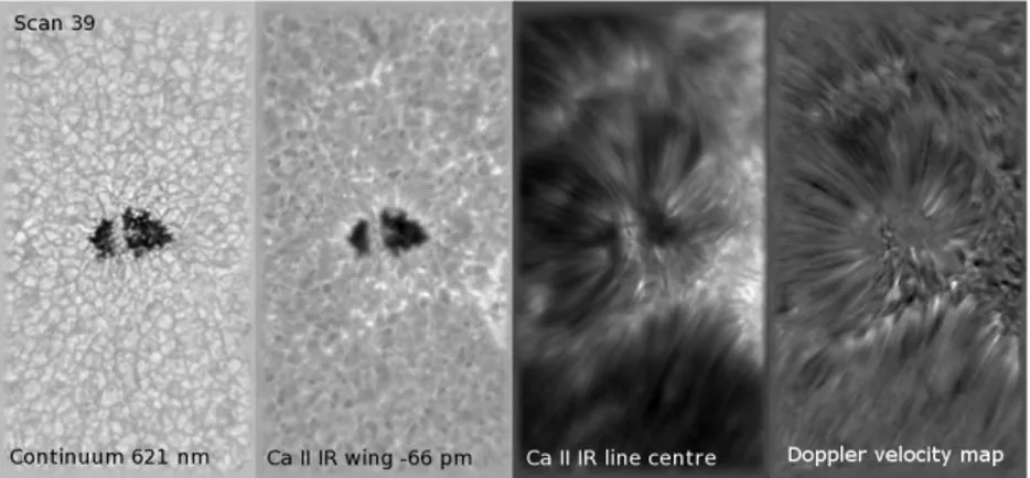
Figure 1. Pore NOAA 11005, full FOV 38′′× 71′′.5. North is on the top, west on the left. From left to right: continuum 621 nm, Ca II 854.2 nm blue wing intensity, line centre intensity, Doppler map with velocity range from −2.3 km s−1 (black, toward the observer) to 4.7 km s−1 (white, away from the observer).
Figure 2. Time-averaged Doppler map with contours of zero, −1 and 1 km s−1. 3. Results
Examples of intensity maps in the continuum 621 nm, blue wing and centre of the line Ca II 854.2 nm and a Doppler map are shown in Fig. 1. Oscillations and waves are filtered out from these images. A filamentary structure around the pore, composed of radially oriented bright and dark fibrils, is clearly seen in the line-centre intensity and Doppler maps. The area and shape of the filamentary structure are identical in all pairs of the line-centre intensity and Doppler images in the time series. The fibrils begin immediately at the umbral border and in many cases continue till the border of the filamentary structure. Their lengths are identical in the Doppler and intensity maps. However, the fibrils seen in the line centre are spatially uncorrelated with those in the Doppler maps.
Concentric running waves originating in the centre of the pore are observed in the unfiltered time series of the line-centre intensity and Doppler images. They propagate through the filamentary structure to the distance 3000–5000 km from the visible border of the pore with a typical speed of 10 km s−1. These waves are very similar to running penumbral waves observed in the penumbral chromosphere and in superpenumbrae of developed sunspots [16].
The subsonic-filtered time series of Doppler maps was averaged in time to obtain a spatial distribution of mean line-of-sight (LOS) velocities around the pore. The result is shown in Fig. 2 together with contours of zero, −1 and 1 km s−1. We can see from the figure that the inner part of the filamentary structure contains a positive LOS velocity (away from us, a downflow), while the outer part, located mostly on the limb side, shows a negative LOS velocity (toward us, an upflow). Taking into account the heliocentric angle θ = 23◦ and the fact that the plasma moves along magnetic field lines forming a funnel, the negative LOS velocity is only partly caused by real upflows but mostly by horizontal inflows into the pore. The picture of plasma moving toward the pore and flowing down in its vicinity is consistent with the inverse Evershed effect observed in the sunspots’ superpenumbra.
All these facts are leading to the conclusion that the filamentary structure observed in the chromosphere above the pore is equivalent to a superpenumbra of a developed sunspot. The missing correlation between the fibrils seen in the line centre and those in the Doppler maps fur-ther supports this conclusion, because, according to [17], flow channels of the inverse Evershed effect are not identical with superpenumbral filaments.
A strong granular LB separates the two umbral cores of the pore. It is the brightest feature inside the pore in the photosphere as well as in the chromosphere, where it is by factor of 1.3 brighter than the average brightness in the FOV. The granular structure of the LB is preserved at all heights, from the photospheric continuum level to the formation height of the Ca II line centre. It is interesting that while a typical pattern of reverse granulation, observed in the Ca II wings, appears outside the pore in the middle photosphere (h ≃ 250 km), the LB is always composed of small bright granules separated by dark intergranular lanes (Fig. 1). A feature-tracking technique was applied to correlate the LB granules in position and time at different heights in the atmosphere. A correlation was found between the photospheric LB granules in the continuum and Ca II wings (correlation coefficient 0.46). On the other hand, there is no correlation between the chromospheric LB “granules” observed in the Ca II line centre and the photospheric ones in the wings and continuum.
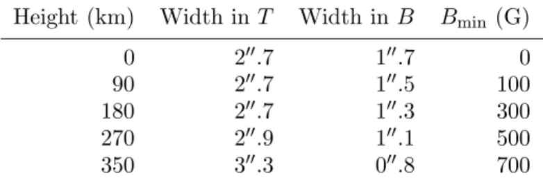
The feature-tracking technique has shown that the mean size of the LB granules increases with height from 0′′.45 in the continuum to 0′′.50 in the Ca II wings and 0′′.54 in the Ca II line centre. Similarly, the average width of the LB increases with height from 2′′ (continuum) to 2′′.5 (Ca II wings) and 3′′ (Ca II line centre). On the other hand, it can be expected that the width of the LB magnetic structure decreases with height due to the presence of magnetic canopy. The complementary HINODE observations in two spectral lines Fe I 630.15 and 630.25 nm made it possible to obtain vertical stratification of temperature and magnetic field strength in the LB photosphere, using the inversion code SIR [18]. The results, summarised in Table 1, show that the width of LB in temperature maps really increases with height, while the width of the LB magnetic structure decreases and the magnetic field strength increases, confirming the magnetic canopy configuration.
Table 1. Widths of the light bridge measured in temperature and magnetic field at different geometrical heights in the photosphere. Bmin is the minimum magnetic field strength in the light bridge.
Height (km) Width in T Width in B Bmin (G)
0 2′′.7 1′′.7 0
90 2′′.7 1′′.5 100
180 2′′.7 1′′.3 300
270 2′′.9 1′′.1 500
350 3′′.3 0′′.8 700
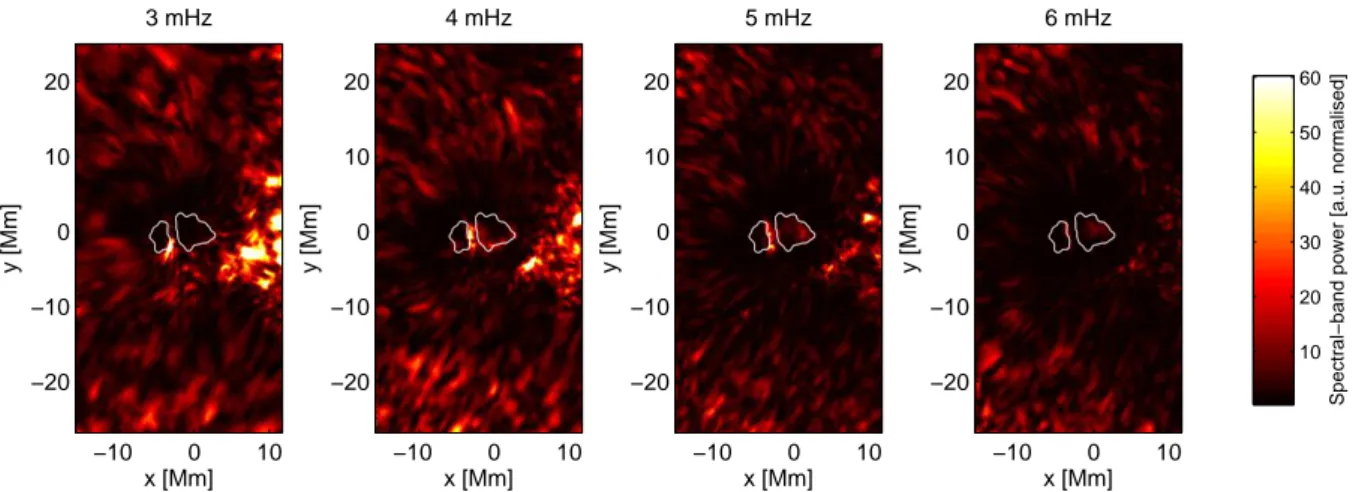
Power spectra of chromospheric oscillations were calculated using the unfiltered time series of the Ca II line-centre intensity and Doppler images. Power maps derived from the Doppler velocities at frequencies 3–6 mHz are shown in Fig. 3. At the LB position, we can see a strongly enhanced power around 3–5 mHz, comparable with that in a plage near the eastern border of the pore A similar power enhancement was reported in [19]. Usually, low-frequency oscillations do not propagate through the temperature minimum from the photosphere to the chromosphere due to the acoustic cut-off at 5.3 mHz [20]. To explain our observations, we assume that the low-frequency oscillations leak into the chromosphere along an inclined magnetic field [19,21], which is present in the LB and in the plage. The inclined magnetic field in the LB is verified by inversions of the full-Stokes Fe I 617.33 nm profiles [10]. The inclination angle, extrapolated to the height of the temperature minimum, is 40◦–50◦ to the west thanks to inclined magnetic field lines at the periphery of the larger (eastern) umbral core. These field lines pass above the magnetic canopy of the LB.
x [Mm] y [Mm] 3 mHz −10 0 10 −20 −10 0 10 20 x [Mm] y [Mm] 4 mHz −10 0 10 −20 −10 0 10 20 x [Mm] y [Mm] 5 mHz −10 0 10 −20 −10 0 10 20 x [Mm] y [Mm] 6 mHz −10 0 10 −20 −10 0 10 20
Spectral−band power [a.u. normalised]
10 20 30 40 50 60
Figure 3. Power maps of Doppler velocities at frequencies 3–6 mHz. The contours outline the boundaries of the pore and light bridge, observed in the continuum.
Following [22], we estimate the acoustic energy flux in the LB chromosphere and compare it with the flux in the “quiet” region. The observed Doppler velocities are used for this purpose. With the estimated magnetic field inclination of 50◦, the effective acoustic cut-off frequency decreases to the value of 3 mHz in the LB. The total calculated acoustic power flux is 550 W m−2 in the LB, while only 110 W m−2 in the “quiet” chromosphere. These results seem to be lower than 1840 W m−2 presented in [22] but one has to bear in mind that this value was obtained for the photosphere, where the power of the acoustic oscillations must be higher than in the chromosphere.
4. Discussion and conclusions
We studied the photosphere and chromosphere above a large solar pore with a granular LB using spectroscopic observations with spatial resolution of 0′′.3–0′′.4 in the line Ca II 854.2 nm and photospheric Fe I lines. We have shown that in the chromospheric filamentary structure around the pore, observed in the Ca II line core and Doppler maps, the inverse Evershed effect and running waves are present. Chromospheric fibrils seen in the intensity and Doppler maps are spatially uncorrelated. From these characteristics and from the morphological similarity of the filamentary structure to superpenumbrae of developed sunspots we conclude that the observed pore has a kind of a superpenumbra, in spite of a missing penumbra in the photosphere.
A special attention was paid to the granular LB that separated the pore into two umbral cores. The magnetic canopy structure [6] is confirmed in this LB. In the middle photosphere (h ≃ 250 km, Ca II wings), the reverse granulation is seen around the pore but not in the LB. The reverse granulation is explained by adiabatic cooling of expanding gas in granules, which is only partially cancelled by radiative heating [23]. In the LB, hot (magneto)convective plumes at the bottom of the photosphere cannot expand adiabatically in higher photospheric layers due to the presence of magnetic field and the radiative heating dominates, forming small bright granules separated by dark lanes. The positive correlation between the LB structures in the continuum and Ca II line wings indicates that the middle-photosphere structures are heated by radiation from the low photosphere. Since the mean free photon path in the photosphere is larger than 1′′ for h > 120 km, the LB observed in the line wings is broader and its granules are larger than in the continuum due to the diffusion of radiation.
In the middle chromosphere (h ≃ 1300 km, Ca II centre), the LB is the brightest feature in the pore and it is brighter by factor of 1.3 than the average intensity in the FOV. Since the
height in the atmosphere is well above the temperature minimum, the radiative heating cannot be expected. The heating by acoustic waves seems to be a candidate, because the acoustic power flux in the LB is five times higher than in the “quiet” chromosphere. To check this possibility, we have to compare the acoustic power flux with the total radiative cooling. An average profile of the Ca II line in the LB was used to derive a simple semi-empirical model based on the VAL3C chromosphere [24], with the temperature increased by 3000 K in the upper chromospheric layers (h > 900 km). The net radiative cooling rates were calculated using this model. The resulting height-integrated radiative cooling is approximately 6700 W m−2 in the LB chromosphere and 3000 W m−2 in the “quiet” chromosphere. The acoustic power fluxes (550 W m−2 and 110 W m−2, respectively) are by an order of magnitude lower than the estimated total radiative cooling, so that the acoustic power flux does not seem to provide enough energy to reach the observed LB brightness.
Acknowledgments
This work was supported by the Czech Science Foundation under grants P209/12/0287 and P209/12/P568 and by the project RVO:67985815 of the Academy of Sciences of the Czech Republic. The Dunn Solar Telescope is located at the National Solar Observatory, operated by AURA for the National Sience Foundation. HINODE is a Japanese mission developed and launched by ISAS/JAXA, with NAOJ as domestic partner and NASA and STFC (UK) as international partners. It is operated by these agencies in cooperation with ESA and NSC (Norway).
References
[1] Simon G W and Weiss N O 1970 Solar Phys. 13 85
[2] Rucklidge A M, Schmidt H U and Weiss N O 1995 MNRAS 273, 491 [3] Keppens R and Mart´ınez Pillet V 1996 Astron. Astrophys. 316 229
[4] S¨utterlin P 1998 Astron. Astrophys. 333 305
[5] Sobotka M 1997 1st Advances in Solar Physics Euroconference, Advances in the Physics of Sunspots, ed
B Schmieder, J C del Toro Iniesta and M V´azquez, ASP Conference series Vol 118 p 155
[6] Jurˇc´ak J, Mart´ınez Pillet V and Sobotka M 2006 Astron. Astrophys. 453 1079
[7] Berger T E and Berdyugina S V 2003 Astrophys. J. 589 L117
[8] Alissandrakis C E, Dialetis D, Mein P et al. 1988 Astron. Astrophys. 201 339 [9] Cavallini F 2006 Solar Phys. 236 415
[10] Sobotka M, Del Moro D, Jurˇc´ak J and Berrilli F 2012 Astron. Astrophys. 537 A85
[11] Viticchi´e B, Del Moro D, Criscuoli S and Berrilli F 2010 Astrophys. J. 723 787 [12] Kosugi T, Matsuzaki K, Sakao T et al. 2007 Solar Phys. 243 3
[13] Tsuneta S, Ichimoto K, Katsukawa Y et al. 2008 Solar Phys. 249 167
[14] Cauzzi G, Reardon K P, Uitenbroek H et al. 2008 Astron. Astrophys. 480 515
[15] Garcia A, Klvaˇna M and Sobotka M 2010 Cent. Eur. Astrophys. Bull. 34 47
[16] Christopoulou E B, Georgakilas A A and Koutchmy S 2000 Astron. Astrophys. 354 305 [17] Tsiropoula G, Alissandrakis C E, Dialetis D and Mein P 1996 Solar Phys. 167 79 [18] Ruiz Cobo B and del Toro Iniesta J C 1992 Astrophys. J. 398 375
[19] Stangalini M, Del Moro D, Berrilli F amd Jefferies S M 2011 Astron. Astrophys. 534 A65 [20] Fossat E, Regulo C, Roca Cortes T et al. 1992 Astron. Astrophys. 266 532
[21] Jefferies S M, McIntosh S W, Armstrong J D et al. 2006 Astrophys. J. 648, L151
[22] Bello Gonz´alez N, Flores Soriano M, Kneer F and Okunev O 2009 Astron. Astrophys. 508 941
[23] Cheung M C M, Sch¨ussler M and Moreno Insertis F 2007 Astron. Astrophys. 461 1163