ALMA MATER STUDIORUM
UNIVERSITÁ DI BOLOGNA
SCUOLA DI SCIENZE
Corso di Laurea Magistrale in Analisi e Gestione Ambientale
"
Dynamics of inorganic carbon and carbonate saturation in the Gulf of Cádiz (SW Spain)”
Tesi in Prevenzione e Controllo dell’Impatto Ambientale
Relatore
Dott.ssa Roberta Guerra Tesi di Laurea di
Controrelatore Maria Giuseppina Zuzolo
Prof.re Daniele Fabbri
Correlatori
Prof.re Jesus M. Forja Pajares Prof.ssa Teodora Ortega Dìaz
III sessione
Anno Accademico 2014-2016
2
Indice
A MI MISMA 3
“CAMINANTE SON TUS HUELLAS 3
EL CAMINO Y NADA MAS; 3
CAMINANTE, NO HAY CAMINO 3
SE HACE CAMINO AL ANDAR. “ 3
1. INTRODUCTION 4
1.1 THE OCEANS AND CARBON DIOXIDE: ACIDIFICATION PROCESS AND THE GLOBAL CHANGE 4
1.2 CARBONATE CHEMISTRY IN THE AQUATIC SYSTEM 8
2. CALCIUM CARBONATE: CHEMICAL PROCESSES, FUNCTIONS OF CALCIFICATION AND
SATURATION STATE 14
3. AIM OF THIS STUDY 20
2. THE STUDY AREA 21
3. MATERIALS AND METHODS 23
3.1 FIELD SAMPLING 23
3.2. PHYSICAL-CHEMICAL CONDITION 24
3.3 TOTAL ALKALINITY 25
3.4. THE CARBON SPECIATION 26
4. RESULTS 27
4.1 OCEANOGRAPHIC VARIABLES 27
4.2. BIOCHEMICAL VARIABLES 4
5. DISCUSSION 18
5.1 HYDROGRAPHY OF THE GULF OF CÁDIZ AND CARBONATE SYSTEM IN RELATION TO DIFFERENT
WATER MASSES IN THE GULF OF CÁDIZ 18
5.2 SEASONAL VARIATION OF TA, DIC, PH AND ΩCA 27
6. FINAL REMARK 32
7. CONCLUSIONS 33
3
A MI MISMA
“CAMINANTE SON TUS HUELLAS EL CAMINO Y NADA MAS;
CAMINANTE, NO HAY CAMINO
4
1. INTRODUCTION
1.1 THE OCEANS AND CARBON DIOXIDE: ACIDIFICATION PROCESS AND THE GLOBAL CHANGE
In 1896 Svante A. Arrhenius claimed that the increase of emissions from fossil fuel-burning into the atmosphere could lead or accelerate global warming (Arrhenius, 1896) and established a relationship between atmospheric carbon dioxide and temperature. Only in the last four decades (Broecker, 1975), the phenomenon of climate change has been observed and has its origins in the increased atmospheric emissions of greenhouse gases, such as carbon dioxide(CO2), methane (CH4)
and nitrous oxide (N2O) and water vapour. These gases have the property of absorbing and re-emitting
the infrared radiation (IR), which is what makes CO2 an effective trap-heat greenhouse gas. In this
way, these molecules gain extra kinetic energy, which may then be transmitted to other molecules and causes general heating of the atmosphere
The greenhouse effect works like this: First, the sun’s energy enters the top of the atmosphere as shortwave radiation and makes its way down to the ground without reacting with the greenhouse gases. Then the ground, clouds, and other earthly surfaces absorb this energy and release it back towards space as longwave radiation. As the longwave radiation goes up into the atmosphere, it is absorbed by the greenhouse gases. The greenhouse gases then emit their radiation (also longwave), which will often keep being absorbed and emitted by various surfaces, even other greenhouse gases, until it eventually leaves the atmosphere. Since some of the re-emitted radiation goes back towards the surface of the earth, it warms up more than it would if no greenhouse gases were present (Figure 1). IR build-up in the lower layers of the atmosphere ultimately causes heating of this , as well as the earth's surface, causing the phenomenon known as global warming.
Anthropogenic greenhouse gas emissions have increased since the pre-industrial era, driven largely by dramatic changes in the economic, social and technological sectors. Since then, their effects have been detected throughout the climate system, and are likely to have been the dominant cause of the observed warming since the mid-20th century.
5
Figure 1. The Greenhouse Effect. Image captured by http://climate.ncsu.edu/edu/k12/.GreenhouseEffect
Recently, National Administration of Department of Aeronautics and Aeronautical National (NASA, National Aeronautics and Space Administration) has conducted a study on air bubbles trapped in ice that allowed to analyse how the earth and climate change have been modified over time. By this work emerged that levels of carbon dioxide (CO2) in the atmosphere are higher than they have ever been
at any time in the past 400,000 years. During ice ages, CO2 levels were around 200 parts per million
(ppm), and during the warmer interglacial periods, they hovered around 280 ppm. In 2013, CO2 levels
surpassed 400 ppm for the first time in recorded history (Figure 2). This recent relentless rise in CO2
shows a remarkably constant relationship with fossil-fuel burning, and can be well accounted for based on the simple premise that about 60 percent of fossil-fuel emissions stay in the air (http://climate.nasa.gov/climate_resources/24/).
Great importance has been the creation of Intergovernmental Panel on Climate Change (IPCC), the leading international body for the assessment and the current state of climate change in 1988; thanks to the IPCC more attention has been driven on climate change and the negative effects it has on the surface temperature, vapour in the atmosphere , precipitation, ice cover , the frequency of extreme event , the sea level and changes in ocean chemistry Synthesis(IPCC,2014).
The anthropogenic CO2 emitted into the atmosphere is largely captured by natural systems
such as the terrestrial biosphere and oceans. Recent studies have estimated that in the past 200 years, the oceans have absorbed 525 billion tons of carbon dioxide from the atmosphere, or nearly half of the fossil fuel carbon emission over this period (Orr et al. 2005, Sabine et al. 2004).
6
Figure 2. Register of annual concentrations of atmospheric CO2 for 800,000 years, conducted on air bubbles trapped in ice by the Administration of Department of Aeronautics and Aeronautical National. Image obtained from http://climate.nasa.gov/climate_resources/24/.
The oceans cover over two-thirds of the Earth’s surface. They play a vital role in global biogeochemical cycles, contribute enormously to the planet’s biodiversity and provide a livelihood for millions of people. Initial evidence shows that the surface waters of the oceans, which are slightly alkaline, are already becoming more acidic: this process is known as of ocean acidification (
Figure 3).
Figure 3. Times series of atmospheric at Manua Loa and surface ocean pH and pCO2 at ocean station Aloha in the subtropical North Pacific Ocean. Mauna Loa data: Dr. Pieter Tans, NOAA/ESRL; HOTS/Aloha data: Dr. David Karl, University of Hawaii (modified after Feely, 2008).
The absorption of anthropogenic CO2 has caused a decrease on surface-ocean pH of ∼0.1 units, from∼8.2 to ∼8.1 (Zeebe, 2012). Surface-ocean pH has probably not been below ∼8.1 during the past 2 million years (Hӧnisch et al. 2009). This value may seem small; however this change represents an increase of about 30% in acidity, measured as hydrogen ion concentration (The Royal Society 2005). The increase of acidification will have significant effects on the marine system. If CO2
7
emissions continue unabated, surface-ocean pH could decline by approximately 0.7 units by the year 2300 (Zeebe et al. 2008). Oceans also play a significant role in the regulation of global temperature and thus they affect a range of climatic conditions and other natural processes on the Earth (Zeebe et al,2001).
The Earth’s climate is currently undergoing changes as a result of global warming, which is impacting many chemical and biological processes( Figure 4) shows the projected rise in temperature through 2100, compared to the rise in temperature we have already experienced since 1900 (the “thermometer” on the right shows warming since the late 1800s). On average, temperatures have risen less than one degree since then. The highest projections of greenhouse gas emissions, known as “Representative Concentration Pathways 8.5” (RCP8.5), indicate that temperatures could rise a full four degrees Celsius above recent temperatures. But if we’re aggressive about mitigating the effect of climate change, we could wind up in a low-emission RCP2.6 scenario of a one- to two-degree temperature rise.
Figure 4. The projected rise in temperature through 2100, compared to the rise in temperature have already experienced since 1900. Image from Pachauri, R.K, et al. (2014)
Carbon dioxide in the atmosphere is chemically an unreactive gas but, when it is dissolved in seawater, it becomes more reactive taking part in several chemical, physical, biological and geological reactions, many of which are complex (The Royal Society, 2005).
When CO2 dissolves in seawater forms a weak acid, called carbonic acid (H2CO3). Part of the acidity is neutralised by the buffering effect of seawater, but the overall impact is to increase the
8
acidity that consequently decreases the concentration of the carbonate ion, whereas the bicarbonate ion ([HCO3]) increases.
The pH of the ocean is also controlled by the temperature of the surface oceans and upwelling of CO2-rich deep water into the surface waters in upwelling areas (The Royal Society 2005).
The solubility of CO2 depends on the temperature so that low surface water temperatures increase the CO2 uptake, while surface warming drives its release. When CO2 is released from the oceans at constant temperatures, pH increases. The concentration of carbon dioxide is higher in deep ocean water because there is no photosynthesis to remove carbon dioxide from the water. Animal respiration and scavenger decomposition also increase the level of carbon dioxide in deep water. Since carbon dioxide solubility in ocean water increases with decreasing temperature and increasing pressure, this allows deeper water to store more carbon dioxide.
One of the most important implications of the changing acidity of the oceans is the effect on many marine photosynthetic organisms and animals, such as corals that make shells and plates using calcium carbonate (CaCO3). This process is known as ‘calcification’ and it is important for the biology and survival of several marine organisms. Calcification is impeded progressively by to decrease of pH and declining[CO3−2]. Consequently the stability of calcium carbonate is reduced.
However, the complexity of the marine biogeochemical processes and the lake of the complete Knowledge of the effect on oceanic CO2 chemistry have led to difficulties in predicting the consequences for marine life. It has also been difficult to set the appropriate threshold levels for a tolerable pH change (Zeebe et al.,2008). For the complete understanding of the effects of acidification, we need to assess all the aspects of the forcing of the marine CO2 system. Model results have shown that the high latitude oceans will be the first to become undersaturated with respect to calcite and aragonite (Orr et al,2005)
1.2 CARBONATE CHEMISTRY IN THE AQUATIC SYSTEM
The reactions that take place when carbon dioxide dissolves in water can be represented by thermodynamic equilibrium where gaseous carbon dioxide [CO2(g)] and [CO2] are related by Henry’s law:
CO2 (g) CO2 (aq)
CO2 (aq) + H2O(l) H (aq) +𝐻𝐶𝑂3− (aq)
The equilibrium relationships between the concentrations of these various species can then be written as:
K0= CO2 (g) = [CO2]
9
K2=HCO−3 =CO2-3+ H+
where K0 is the temperature- and salinity-dependent solubility coefficient of CO2 in seawater (Weiss 1974). The concentration of dissolved CO2 and the fugacity of gaseous CO2, fCO2, then obey the equation [CO2] = K0 ×fCO2, where the fugacity is virtually equal to the partial pressure, pCO2 (within ∼1%). The dissolved carbonate species react with water, hydrogen ions (pH = −log([H+])), and hydroxyl ions and are related by these equilibria:
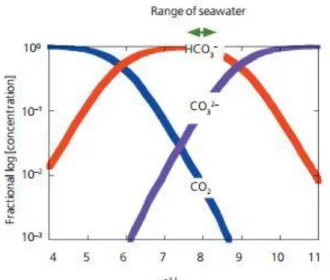
The pK∗s [ = −log(K∗)] of the stoichiometric dissociation constants of carbonic acid in seawater are pK1∗ = 5.94 and pK∗2 = 9.13 at temperature Tc = 15◦C, salinity S = 35, and surface pressure P = 1 atm (Prieto & Millero 2001). At a typical surface-seawater pH of 8.2, the speciation between [CO2],[𝐻𝐶𝑂3−], and [CO32-].In the Figure 5 is showed the distribution of carbonate species as
a fraction of total dissolved carbonate in relation to solution pH.
Figure 5. The distribution of carbonate species. Extract by Zeebe et all,2005
The concentrations of the individual species of the carbon dioxide system are ([CO2],[𝐻𝐶𝑂3−],
and [CO32-]). They can however be obtained from experimental parameters [pH, partial pressure of
CO2 (pCO2 ), total dissolved inorganic carbon (DIC) and total alkalinity (AT)] along with the utilization of thermodynamic constants. In order to characterize the carbonate system, at least two parameters are required. As an example, consider the case in which DIC and [H+] (i.e. pH) have been obtained by direct measurement.
The total inorganic carbon (CT, or TIC) or dissolved inorganic carbon (DIC) is the sum of inorganic carbon species in a solution. The inorganic carbon species include carbon dioxide, carbonic acid, bicarbonate anion, and carbonate:
10
The concentrations of the different species of DIC (and which species is dominant) depends on the pH of the solution.
Alkalinity is an experimental value that has been used widely together with pH in the calculation of dissolved inorganic carbon speciation in sea water. Essentially, it consists in the measurement of the quantity of strong acid necessary to transform all inorganic carbon present to CO2. Because there are a number of acid- base equilibriums in sea water apart from those involved in the carbonate system, the total alkalinity (AT) can be expressed in a general form as :
AT= [Weak Acids] – [Weak Protonised Acids] + [OH-] – [H+]
The total alkalinity of a sample of sea water is a form of mass-conservation relationship for hydrogen ion. It is rigorously defined (Dickson, 1981) as “. . . the number of moles of hydrogen ion equivalent to the excess of proton acceptors (bases formed from weak acids with a dissociation constant K ≤ 10–4.5 at 25°C and zero ionic strength) over proton donors (acids with K > 10–4.5) in 1 kilogram of sample.” Thus
AT= [𝐻𝐶𝑂3−]+2[CO32-]+[𝐵(𝑂𝐻)4−]+[𝑂𝐻−]+[HPO2−4 ]+2[𝑃𝑂43−]+[SiO(𝑂𝐻)3−]+[NH3]+[ 𝐻𝑆−]-[ 𝐻+]F
−[𝐻𝑆𝑂4− ] − [HF] − [H3 PO4];
The concentrations are total concentration and include the multiple ionic associations formed by these species in sea water.
This expression is currently widely accepted for alkalinity in sea water. It is required for
carrying out inorganic carbon speciation in complex marine system. When the expression is applied
to oceanic waters, it simplified to:
AT= [𝐻𝐶𝑂3−]+ ]+2[CO32-]+[𝐵(𝑂𝐻)4−]
The hydrogen ion concentration in sea water is usually reported as pH: pH = −log[H+ ]
Although the concept of a total hydrogen ion concentration is somewhat confusing, it is needed to define acid dissociation constants accurately in sea water (Dickson, 1990). Total hydrogen ion concentration is defined as:
11
where [H+]F is the free hydrogen ion concentration, ST is the total sulphate concentration ([SO42]+[𝐻𝑆𝑂4− ] and KS is the acid dissociation constant for 𝐻𝑆𝑂4−. At pH values above 4, previous equation can be approximated as:
[H +] =[H+]F + [𝐻𝑆𝑂 4−]
The pH scale and the corresponding analysis of the proton transfer reactions in sea water constitute one of the most controversial issues in marine chemistry. This is due to the current use of 3 distinct scales for the expression of the hydrogen ion concentration each with their own corresponding dissociation constant for a particular proteolytic species (Dickson, 1984) (
Table 1).
Table 1.Nomenclature proposed by UNESCO (1987) for the pH scale. Where K´, K* and Km are apparent, stoichiometric and in terms of molalities respectively
pH Scale [H+] pH K NBS aH (NBS) pH (NBS) K´
Total hydrogen ion concentración (mol / Kg-soln)
[H+]T pHT K*
Free hydrogen ion concentration (mol / Kg-H)
mH pmH Km
The difference between the distinct pH scales owes fundamentally to the different regulating solutions used for calibration of the pH meters. The international scale for pH is based on standard diluted solutions of low ionic strength as put forward by the National Bureau of Standards (NBS) (pH 4.00 and pH 7.02) and represents a normalized pH scale. This is without doubt the most commonly used scale for pH measurement in natural water bodies of low ionic strength such as rivers, lakes and aquifers (Bates 1973, 1975; Covington et al., 1985) as well as being the scale utilised by the majority marine studies.
The electro-chemical measurement of pH is affected by the state of the electrode and the variation in liquid union potential of the reference electrode when it passes from one medium to another, for the example standard solution and the sample. The value increases when the difference in composition between the two mediums is accentuated. This effect is patent in sea water, since its ionic strength (0.7 M) is different from the NBS standard solutions (I< 0.1M). The suitability of
12
applying this pH scale in the marine environment has been questioned by various authors (Bates and Culberson, 1977; Dickson, 1984; UNESCO, 1987; Dickson, 1993).
The problem of the low reproducibility in the measurement of pH in sea water is currently solved using a standard solution of similar ionic strength. These solutions are used on scales known as “overall/total concentration” and “hydrogen ion free concentration” (pHT and pmH, respectively).The overall/total scale was defined by Hanson (1973) in terms of the total hydrogen ion concentration (H+ + HSO4-) per kg of sea water. Following this, Bates and Macaskill (1975) defined the pmH scale in hydrogen free ion molalities. This scale is converted directly to the overall/total scale by taking the bisulphate ion into account.
Dickson and Riley (1979) defined the Sea Water Scale (SWS), which differentiates itself from the overall scale by including the concentration of hydrogen fluoride. Currently, the use of this scale isn’t widespread since the equilibrium constant in water for hydrogen fluoride is not well known. Nevertheless, the error produced by ignoring fluoride is negligible. Dickson (1993) defended the use of the overall/total scale and found that the difference in the hydrogen ion concentration given by the “overall/total” when compared to the “Sea Water” scale was around 2-3%.
The last three scales mentioned use standard solutions made up of artificial sea water and as a buffer system, an equimolar blend of methyl-amine and tris-hydroxymethyl-methyl-ammonium chloride, commonly known as TRIS and TRIS·HCl. These solutions have the advantage of not creating a significant variation in liquid union potential between the calibration solution and the samples.
The free and total hydrogen ion concentration scales are related by the following expression (Culberson, 1981):
pHT = pHF – log(1+ HSO4 [SO42-])
Where HSO4 is the association constant for the formation of HSO4-: HSO4 = [HSO4-] / [H+] · [SO42-]
The value of HSO4 has been determined in sea water at a range of temperatures by various researchers (e.g. Khoo et al., 1977; Bates and Calais, 1981; Millero, 1983).
The pH scales (NBS) and the total hydrogen ion concentration, are expressed in terms of one another via the apparent hydrogen ion activity (fHT), which is defined as:
13
T H T H H a f where aH is the apparent hydrogen ion activity and [H+]T is the total hydrogen ion concentration (H+ + HSO4-) in moles per kilogramme of sea water (UNESCO, 1985). The relation between the NBS and SWS scales is the same as that described, with the only difference being that for the total proton concentration, H+, HSO4- and HF are considered. In the same way, the apparent activity coefficient for the free hydrogen ion concentration (fHF) is:
1 S 1000
m a f H H F H This equation relates the NBS and free hydrogen ion concentration (pmH) scales where pmH is the apparent hydrogen ion activity.
The partial pressure of carbon dioxide in an aquatic system is described by the Henry's law:
pCO2= K0[CO2]ac
Since CO2 has not an ideal behaviour using the fugacity in place of the partial pressure:
fCO2 =f pCO2
It assumes f=0.997 at 25°C and that CO2 has an ideal behaviour , and then fCO2≈ f pCO2.
Through the use of these two experimental parameters and the use of the dissociation of carbonic acid , it is possible to determine all the behaviours that describe the carbon in the seawater system
Some of the main basics of seawater carbonate chemistry are illustrated in the Figure 6 as total dissolved inorganic carbon (DIC), total alkalinity (TA), and [CO2] at temperature T = 15 °C, salinity S = 35, and pressure P = 1 atm .Contours indicate lines of constant [CO2] in μmol kg−1. Invasion and release of CO2 into/from the ocean changes only TCO2, whereas photosynthesis and respiration also slightly change TA owing to nitrate uptake and release. CaCO3 formation decreases T CO2 and TA in a ratio of 1:2, and, counterintuitively, increases [CO2], although the total inorganic carbon concentration has decreased. CaCO3 dissolution has the reverse effect. Modified from Broecker & Peng (1989) and Zeebe & Wolf-Gladrow (2001).
In the carbons equilibrium the temperature and salinity are so important particularly at the surface, in fact CO2 is less soluble at higher temperatures, leading to outgassing to the atmosphere and hence locally reduced TCO2.Conversely, CO2 uptake takes place predominantly in colder waters, and TCO2 is higher.
14 Figure 6. Basics of seawater carbonate chemistry as total dissolved inorganic carbon (DIC), total alkalinity (TA), and [CO2] at temperature T = 15 °C, salinity S = 35, and pressure P = 1 atm. Image captured
by Zeebe et al,2012
2. CALCIUM CARBONATE: CHEMICAL PROCESSES, FUNCTIONS OF CALCIFICATION AND SATURATION STATE
Important issues have indicated the important role of calcium carbonate in the context of ocean acidification and calcifies.
Several studies have evidenced that biogenic calcification will decline and CaCO3 dissolution will increase under rising atmospheric CO2 and lowered seawater pH (Kleypas et al., 1999). Calcium carbonate becomes more soluble with decreasing temperature and increasing pressure, and hence with ocean depth.
The biological production and dissolution of CaCO3 in the ocean result in changes in TA in the water column according to the following reaction:
CaCO3 + H2O + CO2 Ca2+ + 2HCO-3 .
A change in the balance of this reaction in the ocean would have a significant impact on atmospheric CO2 concentration (Zondervan et al., 2001). Dissolution of CaCO3 particles increases TA in seawater and thus the capacity of the ocean to absorb CO2 from the atmosphere, whereas the production of CaCO3 leads to the opposite consequence (Zeebe et al.,2012)
The mineral CaCO3 derives from shells and skeletons of marine organisms, including plankton, corals and coralline algae, and many other invertebrates. In pelagic environments, carbonates fall through the water column and are either dissolved or deposited in shallow or deep-sea sediments (Feely et al. 2004,Berelson et al. 2007)
15
The formation and dissolution of calcium carbonate (CaCO3) is an important component of the oceanic carbon cycle. The CaCO3 cycle modulates the oceanic dissolved inorganic carbon. Since the settling time of CaCO3 particles is thought to be short if compared to dissolution rates, it was generally believed that much of the carbonate dissolution takes place upon or just beneath the surface of the sediments.
As a consequence of this process, the oceanic CaCO3 export will decrease, which might further weaken its ballast effect for vertical transfer of organic carbon to the deep ocean (Armstrong et al., 2002; Barker et al., 2003).
However, evidence from a variety of sources suggests that as much as 60-80% of net CaCO3 production is dissolved in depths that are above the chemical lysocline, the depth below which the rate of CaCO3 dissolution distinctly increases (Milliman et al., 1999; Francois et al., 2002).
Calcium carbonate exists in two main structures. These are aragonite, which has orthorhombic symmetry in its structure, and calcite, which is trigonal. Both aragonite and calcite are abundant in organisms. However, because of its structure, calcite is less soluble than aragonite (Scott et al, 2009). Usually seawater is supersaturated with constituents for the formation of calcium carbonate (calcite or aragonite). Anyway, in many areas, immediately below the sediment-water interface, the release of protons produced by aerobic degradation processes of organic matter leads to the dissolution of CaCO3.
This is mainly seen in the existence of an increased calcium concentration near the sediment-water interface. At greater depths, the degree of saturation of CaCO3 in the interstitial sediment-water increases due to increased alkalinity producing anaerobic degradation processes of organic matter, primarily the sulphate reduction, which causes the precipitated CaCO3. In coastal areas, where the contributions of organic matter usually high, these processes of dissolution/precipitation of CaCO3 have great relevance (Jahnke y Jahnke, 2000; Mucci et al., 2000).
The carbonate saturation (Ω) depend on the carbonate concentration, pressure, temperature and salinity. Calcite and aragonite are examples of minerals whose solubility increase with decreasing temperature. e aragonite is more soluble, its saturation 𝐶𝑂32− is always higher than that of calcite. These data are plotted in Figure 7, which clearly illustrates the greater importance of pressure over temperature in determining calcium carbonate solubility for both calcite and aragonite. This unusual behaviour is referred to as retrograde solubility. Because of the pressure and temperature effects, calcium carbonate is far more soluble in the deep sea than in the surface waters. Most water masses are not at equilibrium with respect to either calcite or aragonite. The degree to which a water mass
16
deviates from equilibrium for a particular mineral type can be expressed as its degree of saturation, which is defined as :Ca2+
Ω =[𝐶𝑎2+]𝑜𝑏𝑠𝑒𝑟𝑣𝑒𝑑 ×[𝐶𝑂32−]𝑜𝑏𝑠𝑒𝑟𝑣𝑒𝑑
[𝐶𝑎2+]𝑠𝑎𝑡𝑢𝑟𝑎𝑡 ×[𝐶𝑂
32−]𝑠𝑎𝑡𝑢𝑟𝑎𝑡
= 𝐼𝑜𝑛 𝑝𝑟𝑜𝑑𝑢𝑐𝑡 𝐾𝑠𝑝∗
Where [Ca2+]observed and [𝐶𝑂32−]observed are the in situ concentrations in the water mass of interest; 𝐾𝑠𝑝∗ of calcite in seawater of 35 ‰ at 25°C and 1 atm is 10-6.4.Since aragonite is more soluble than calcite, Ωcalcite is always greater than Ωaragonite for a given water mass.
If Ω is greater than 1, the water mass is supersaturated and calcium carbonate will spontaneously precipitate until the ion concentrations decrease to saturation levels. When Ω is less than 1, the water mas is under saturated. If calcium carbonate is present, it will spontaneously dissolve until the ion product rises to the appropriate saturation value. Although calcium is a bio intermediate element, it is present at such high concentrations that particulate inorganic carbon (PIC) formation and dissolution causes its concentration to vary by less than 1%. Thus, [Ca2+]observed ≈[Ca2+]saturation it is possible resume Ω as :
Ω= [𝐶𝑂32−]observed
[𝐶𝑂32−]saturation
Figure 7.Saturation concentrations of carbonate ion in seawater as a function of temperature and pressure. Image by Susan M. Labes, 2009
The depth at which dissolution starts to have a significant impact on the sedimentary %CaCO3 is termed the calcite lysocline (Susan M. Libes,2009).
17
Lysocline is defined as the depth in the water column where a critical undersaturation state with respect to aragonite or calcite results in a distinct increase in the CaCO3 dissolution rate (Morse, 1974). For want of a more robust definition, a chemical lysocline is sometimes defined at Ω = 0.8, a value which marks a distinct increase in dissolution rate. The lysocline is the horizon where dissolution becomes first noticeable (a sediment property), and is typically below the calcite saturation horizon (Heiko et all., 2012).
Deeper still, and dissolution becomes sufficiently rapid for the dissolution flux back to the ocean to exactly balance the rain flux of calcite to the sediments. This is known as the calcite (or carbonate) compensation depth (CCD). Because in the real World the boundary in depth between sediments that have carbonate present and those in which it is completely absent is gradual rather than sharp, the CCD is operationally defined, and variously taken as the depth at which the CaCO3 content is reduced to 2 or 10 wt.% ( Ridgwell and Zeebe 2005).
At the CCD the rate of supply of calcite equals the rate of dissolution, and no more calcite is deposited below this depth. In the Pacific, this depth is about 4,5000 below the surface; in the Atlantic, it is about 6,000 m deep. This dramatic variation is due to differences in ocean chemistry. The Pacific has a lower pH and is colder than the Atlantic, so its lysocline and CCD are higher in the water column because the solubility of calcite increases in these conditions.
In the Figure 8 the relationship between CCD, sediment CaCO3 content (dotted black line), carbonate accumulation rate (blue line) and lysocline, in comparison with cumulative ocean floor hypsometry (orange line) is showed. The CCD, a sediment property, is defined as where carbonate rain is balanced by carbonate dissolution. Previously, it has been operationally defined to coincide with a fixed content of CaCO3 (for example, 10%) in sediments, or where the carbonate accumulation rate interpolates to zero (this second definition is advantageous as it is independent of non-carbonate supply or dilution effects).
18 Figure 8. The position of the CCD and lysocline, and their relationship to ocean bathymetry, carbonate accumulation rate and CaCO3 content. Image Heiko P et al., 2012.
The use [Ca2+ ] to look into the marine CaCO3 cycle is related to the variations of Ca2+ in the ocean interior that are almost solely controlled by CaCO3 formation and dissolution on day‐to‐decade time scales. Ca2+, one of the eleven major ions in seawater, has been recognized to be conservative in the ocean ( Pilson, 1998; Millero, 2006).
Since calcium has a such fundamental role in biotic calcification there have been many studies about its distribution in the oceans. Dyrssen et al.(1968) and Whitfield et al.(1969) proposed a potentiometric titration methods using calcium selective electrodes but results had not have a high shown an high accuracy. However after this study Ruzicka et all (1973) and Lebel and Poisson(1976), developed this method until to get a precision 0.1%.
The aim of this study has been to improve the method of these authors to analyzed the calcium concentration in the open ocean.
It is known that the Ca2+ concentration is relatively small and it has a conservative state in ocean as proposed by Milliman (1993), Balch and Kilpatrick (1996), Pilson(1998) and Berelson et al.,(2007).
However, it is possible to assumed that in costal environments the calcium has a not stable state because of the river input, the rain the biological precipitation of calcium carbonate from the adjacent surface waters of the Gulf and other chemical or physical factors.
A non-conservative calcium state has been observed for some natural systems: the Persian Gulf (Wells,Illing,1964), small hard-water lakes (Wetzel 1966) and shallow carbonate marine environments (Broecker and Takahashi,1966)
19
In the seawater, Ca2+ concentration typically representing only 1% of its ambient concentration,∼10,280 mmol kg−1 at a salinity of 35 (Pilson, 1998). For this reason there is lacke of data.
In support of these claims arguments different studies have been conducted to assess the investigate effects of acidification on carbonate production. It very difficult to evaluate this effect because the baseline estimates of how much carbonate is produced and rains through the water column has been shifting (Berelson et al., 2007).
Milliman (1993) estimated carbonate production in the entire ocean at 5 x10¹³ moles CaCO3 yr-1 ( 0.6 Gt PIC yr-1), which included both neritic and open ocean environments. Later, Milliman et al. (1999) determined carbonate production in the open ocean at 6 x 10¹³ moles CaCO3 yr-1 (= 0.7 Gt PIC yr-1) based on an inventory of alkalinity and the residence time of various water masses.This value was significantly higher than the one estimated with flux into deep traps and lead to the hypothesis that high rates of carbonate dissolution may occur within the water column.
Balch and Kilpatrick (1996) measured carbonate production in the equatorial Pacific and determined a ratio of PIC to POC (particulate organic carbon) production of 9%, which, if globally extrapolated would yield to estimate of carbonate production of 3.5 x 10¹⁴ moles CaCO3 yr-1 (= 4.3 Gt PIC yr-1).
Balch et al. (2007) reevaluated carbonate production from an assessment of satellite-determined parameters, calcification, and photosynthesis rate determinations, and this value is 1.3 x10¹⁴ moles CaCO3 yr-1 (1.6 Gt PIC yr-1).
Recent estimates of both CaCO3 production and export at a global ocean scale were roughly at the same order, at 0.4–1.8 Gt C yr−1, suggesting relatively high carbon export efficiency in the form of inorganic carbon (Berelson et al., 2007).
If the carbonate system is in steady state, the amount produced in the surface water should equal or exceed the amount falling out of the surface ocean (export), and this would equal the sum of what is remineralized and what is buried (Berelson et al.,2007).
The dissolution of one mole of calcium carbonate adds one mole of calcium and two equivalents of alkalinity to the sea water. The concentration of calcium and alkalinity in sea water are, therefore, expected to change in this proportion if other processes which change calcium concentration or alkalinity are absent (Kanamori et all, 1980).
Ca2+ does not suffer from such potential issues. The excess Ca2+ (Ca2+_ex) in the ocean interior, if it exists, can only have originated from CaCO3 dissolution, especially in waters at shallow depth being hardly influenced by hydrothermal inputs (de Villiers and Nelson, 1999). There is
20
conjecture that dissolution or ion change of silicate material in the water might increase Ca2+ in the intermediate water (Tsunogai et al., 1973), however, until now there is no report of such processes. While we also recognize the potential of shallow depth CaCO3 dissolution from many trap studies (e.g., Martin et al., 1993; Honjo et al., 1995; Wong et al., 1999), the magnitude and the causes accounting for shallow‐depth CaCO3 dissolution warrant further examination, in particular in the context of better predicting the response of oceanic buffer capacity to increasing penetrated anthropogenic CO2. We argue that high‐quality Ca2+data from a proper study site with distinguishable preformed waters are required to better examine this shallow‐depth CaCO3 dynamics
3. AIM OF THIS STUDY
The main aim of this work is characterize the Dissolved Inorganic Carbon (DIC) dynamics and the saturation state of calcium carbonate in the north-eastern area of Gulf of Cadiz. The achievement of this aim defines the spatial and temporal distribution of DIC in the study area, as well as the saturation state of CaCO3.
These are the specific aims:
- Quantification of inorganic carbon from pH and total alkalinity measured in samples collected along transects in the gulf of Cadiz and different depths in every stations of sampling.
- Estimation of the saturation state of CaCO3 of calcite and aragonite, and their spatial and temporal variation in the Gulf of Cadiz
- Understanding data obtained considering the specific hydrodynamic and chemical characteristics of water mass and seasonal variations.
Calcium is a major element in seawater, and its concentration changes at ocean level. There are many studies where calcium is calculated from salinity (Pilson, 1998, Shadwick et al.2014). However in coastal areas due to the contribution of the rivers and to processes of CaCO3 dissolution
21
/ precipitation, this element may have variations in its concentration. The second aim of this work is to optimize the measurement of calcium in seawater, allowing a better quantification for future work of the saturation state of CaCO3.
2. THE STUDY AREA
This study was carried out in the nearshore north-eastern shelf of the Gulf of Cádiz (SW Iberian Peninsula), which is a wide basin between the Iberian Peninsula and the African continent where the North Atlantic Ocean and the Mediterranean Sea meet through the Strait of Gibraltar (Figure 9).
Figure 9. Satellite image of Gulf of Cádiz
The Gulf of Cádiz is a domain of considerable interest since it connects the Mediterranean Sea with the Atlantic open ocean and receives the outflowing Mediterranean seawater through the Gibraltar Strait. It therefore plays an important role in the North Atlantic circulation and climate in general (Reid, 1979; Price and O’Neil-Baringer, 1994; Mauritzen et al., 2001). First, in the Gulf of Cadiz there are several water masses mixing to form the ‘‘Atlantic inflow’’ which is responsible for the general oligotrophic and relatively well oxygenated regime of the north-western Mediterranean Sea (Packard et al., 1988; Minas et al., 1991). Second, this area is on the pathway of the ‘‘Mediterranean outflow’’ which thereafter enters to the open ocean and influences the circulation of
22
the North Atlantic and climate in general (Rahmstorf, 1998). The study of the carbon exchange throughout this strait began only a few years ago and it has already been emphasized that the Gulf of Cadiz plays an important role in the carbon cycle of the. eastern North Atlantic (Parrilla, 1998) and the Mediterranean Sea (Dafner et al., 2001).
Only few biogeochemical studies have been done in this area (Minas et al., 1991; Minas and Minas, 1993; Echevarria et al., 2002), especially for the CO2 system (Dafner et al., 2001; Santana-Casiano et al., 2002; González-Dávila et al., 2003).
The Gulf of Cadiz is well documented from a physical point of view (Madelaine, 1967; Zenk, 1975; Ambar et al., 1976; Ochoa and Bray, 1991; Price et al., 1993). The general surface circulation in the Gulf of Cadiz is anticyclonic with short-term, meteorologically induced variations. Hydrodynamics in the Gulf of Cádiz is dominated by the exchange of water masses that occurs in the Strait of Gibraltar, between the Atlantic Ocean and the Mediterranean Sea. Thus the surface water enters the Atlantic Ocean to the Mediterranean, while the masses of water of the Mediterranean, denser, go through the Strait at greater depths (Gascard and Richez, 1985), thus producing a bilayer exchange flow through Strait of Gibraltar (Ochoa and Bray, 1991). This exchange is related to the warm, dry climate of the Mediterranean Sea and its basin has produced a negative water balance, with a predominance of evaporation over precipitation, and that favors the importation of water from outside (Margalef and Albaigés, 1989).
This circulation is maintained in the Gulf of Cádiz, where there are 3 main types of water masses of well characterized. From the surface and even the seasonal thermocline is a body of water of Atlantic origin modified platform-ocean exchanges (Criado-Aldenueva et al., 2006). The presence of NACW in the area is evident below 100 m depth, as described in previous studies (Navarro et al., 2006). This water mass has been categorized in two varieties, such as the warmer Eastern North Atlantic Central Water of subtropical origin (ENACt) and the colder subpolar Eastern North Atlantic Central Water (ENACs) (Ríos 157 et al., 1992; Pollard et al., 1996; Pérez et al., 2001; Alvarez et al., 2005). At shallower depths, NACW is modified by the atmospheric interaction and it has been defined as North Atlantic Surface Water (Gascard and Richez, 1985).
A general movement taking place in the Gulf of Cádiz, we must add the entry of inland water from various rivers, such as the Guadiana, Guadalquivir, Tinto and Odiel.
Another feature that can be highlighted in the Gulf of Cádiz is the existence of upwelling areas in capes of San Vicente and Santa Maria, located in the westernmost part of this area and also form part of the northern branch of outcrop Canary .These are produced by the wind that dominates the area, although Cape Santa Maria is a process rather short time, due to changes in wind patterns (García
23
et al., 2002), leading to higher values biological production. In addition, areas such as the mouth of the Guadalquivir River and the Bay of Cádiz, have the highest values of primary production of the basin (Navarro and Ruiz, 2006).
3. MATERIALS AND METHODS
3.1FIELD SAMPLING
This work is part of the investigation project of the Institute of Oceanography Spanish (IEO), STOCA (Series Temporales de datos Oceanográficos en el Golfo de Cádiz), in partnership with Campus de Excelencia Internacional del Mar (CEI MAR) and the University of Cadiz.
The aims of this project is to establish the effects of global change on the east part of the Gulf of Cádiz (from the Straits of Gibraltar to the mouth of the Guadalquivir River) based on a systematic sampling of radio or defined transect.
Water samples were collected during the STOCA cruises on board of the R/V Alvariño Angeles and Ramon Margalef. The data reported in this work were collected during 4 cruises that took place 28-31 March 2015 (STOCA 5), 15-18 June 2015 (STOCA 6), 15-18 September 2015 (STOCA 7) and 1-4 November 2015 (STOCA 8) 2015.The first two were on aboard the R / V Angeles Alvariño , while the latter on the R / V Ramón Margalef.
In each of the campaigns, three transects perpendicular to coast, were performed. The chosen transect of Guadalquivir was about 45 km, and water depth varied from 5 to 550 m. The chosen transect of Sancti Petri was about 53 km, and water depth varied from 5 to 600 m. The chosen transect of Trafalgar was about 40 km, and water depth varied from 5 to 250 m. Surveys were carried out continuously for 24 h (as long as weather conditions permitted).
Guadalquivir and Sancti Petri transects have six stations each, while Trafalgar has four set points (only for the cruise STOCA 7 5 stations) (Figure 10). At each sampling station STOCA profile CTD- O2 - LADCP was performed and water samples were taken to levels on surface , 25 m, 50 m, 75 m, 125 m and bottom.
Water samples were taken following the protocol described below. The equipment used for hydrographic measurements and sampling of water was Batisonda and rosette system for profiles of the water column while samples are taken at certain levels. Batisonda is integrated in the rosette which currently has 9 bottles of 10 L. We continuously registered currents with acoustic Doppler profiler (LADCP), temperature, salinity and fugacity of CO2 (fCO2) to provide real-time readings via the serial uplink channel.
24 Figure 10. Distribution of transects in the study area . The GD points for the Guadalquivir River, SP for Sancti Petri Channel and TF to Cape Trafalgar
3.2.PHYSICAL-CHEMICAL CONDITION
In order to have a complete knowledge on the physical-chemical and oceanographic conditions of the water column for each cruise it was used the CTD- O2 - LADCP sensor that has continuously recorded salinity (by measuring the conductivity) , temperature and depth ( by pressure meter ). The CTD sensor was associated with Niskins bottles, connected to each other to form a rosette . The Niskin bottles are designed so that they have the lids at the ends . When the probe is immersed in water , the lids of Niskins are open and there is a mechanism that is triggered to close electronically to the different depth chosen. The measured data are analyzed in real time by means of a conductor cable which connects the CTD to a computer on board the ship . Water samples were taken during the rise of the rosette (Figure 11)
25 Figure 11 Rosette incorporated with sensor CTD. Image captured during one of cruises.
3.3TOTAL ALKALINITY
At each station samples were collected to analyse total alkalinity (TA) and pH.
Total alkalinity and pH were measured by endpoint potentiometric titration in an open cell (Metrohm 905) using a combined glass electrode (Metrohm , ref 6028300). The pH was calibrated in the Total pH Scale. The HCl titrant solution (0.1 mol kg-1) was prepared in 0.7 M NaCl, to approximate the ionic strength of the sample, and calibrated against certified reference seawater by A. Dickson ( Scripps Institution of Oceanography , University of California, San Diego, USA , Batch # 128). Accuracy and precision of the TA measurement on CRM was determined ±1.4 μmol kg-1 In Figure 12 a typical titration curve is shown. The inflection points that correspond to the formation of bicarbonate and carbonic acid can be appreciated.
AT was determined from the second equivalence point (Ve2) , and the concentration of acid used in the tritation (CA ) and the volume of sample used ( V0) :
𝐴𝑇 = 𝑉
𝑒2∙ 𝐶
𝐴𝑉
026 Figure 12. Titration curve. The inflection points correspond to two equivalent points.
3.4.THE CARBON SPECIATION
The calcium concentration [Ca2+] is assumed to be conservative and proportional to the salinity, and is largely determined by variations in [CO32−], which can be calculated from DIC and total alkalinity data. Following the determination TA, the pH (on the total scale), DIC and aragonite and calcite saturation state Ω were computed, using the standard set of carbonate system equation with CO2SYS software (Pierrot et al., 2006). The thermodynamic solubility products for aragonite and calcite (KC,A*) are from Mucci (1983) corrected for in situ temperatures and pressures (Millero, 1983).
The expressions for the calculation of the solubility equilibrium for aragonite and calcite are:
5 . 1 3 5 . 0 3 0 · 10 · 1249 . 4 · 07711 . 0 ) 34 . 178 10 8426 . 2 77712 . 0 ( log log S S S T T K KC C 5 . 1 3 5 . 0 3 0 · 10 · 9415 . 5 · 10018 . 0 ) 135 . 88 10 7276 . 1 068393 . 0 ( log log S S S T T K KA A
27
We used the thermodynamic equation and constants for carbon, sulphate and borate of Lueker et al.(2000), Dickson (1990) and Lee at al.,2010, respectively. KC,A was calculated for both calcite and aragonite and the saturation states were given in terms :
ΩC,A = [𝐶𝑂32−] X [Ca2+]
K(C,A)
The value of ΩC,A < 1 represent under saturated conditions, whereas the value of ΩC,A > 1 represent conditions of supersaturation.
The carbonate concentration, [𝐶𝑂32−], is calculated from TCO2, pH, and the values of K1 and K2 for carbonic acid.The effects of pressure on K1 and K2 are from Millero (1995).
The pressure correction for Ksp for calcite is from Ingle (1975) and that for aragonite is from Millero (1979).
We used AT, pH at 15 °C, salinity and sea surface temperature (SST) for each sample and the CO2 calculation program CO2SYS (Lewis and Wallace, 1998) to calculate, total dissolved inorganic carbon (DIC), in situ pH, the carbonate ion concentration [𝐶𝑂32−], and the saturation state of aragonite (ΩA) and calcite (ΩC). The calculations were performed at the total hydrogen ion scale (pH mol/kg-SW) Lee et al. (2010). For KSO4 we used the constant determined by Dickson (1990) and K1, K2 from Lueker et al., 2000.
DIC is defined as the sum of [CO2]+[𝐻𝐶𝑂3−]+ [𝐶𝑂32−] and AT is defined as [𝐻𝐶𝑂3−]+2[𝐶𝑂32−]+ [𝐵(𝑂𝐻3−]+[OH−]−[H+]. KSO4 (Dickson 1990a; Khoo et al. 1977).
4. RESULTS
4.1OCEANOGRAPHIC VARIABLES
Oceanographic [Salinity, S and Temperature, T (°C)] and biochemical variables (carbon system parameters) measured in the Gulf of Cádiz during the four STOCA sampling cruises accomplished in March, June, September and November 2015 (Table 2).
28
The highest values of temperature and salinity were observed in surface waters (~ 25 m top layer) in June and September and June and November, respectively, while lower temperatures were recorded in March. A sudden change of temperature is observed between March and June with a mean difference of about 3-4 °C, while differences between June and September, and September and November are of about 1-2 °C (Table 2).
Temperature decreased and salinity increased with depth, respectively. The thermocline was detected at 100 m depth and consisted of a sudden temperature decrease of about 1°C. Likewise, the halocline has been found at the same depth, extending down to a depth of 300 m, after which salinity started increasing again in deeper waters offshore. A slight increase in salinity was observed offshore in March and September (Figure 13)
Recorded temperatures were significantly different among seasons in the Guadalquivir, Sancti Petri and Trafalgar sampling areas (p < 0.01). In fact, March and November are significantly different, while September and November are not different. Minimum and maximum values were recorded
It is noteworthy that, the highest temperatures were recorded in June and November while in March and September tended to decrease, with the minimum value recorded in spring.
Overall, the oceanographic variables measured during March cruise reflected typical conditions recorded in Winter and June in Spring; conversely, September reflected the Summer conditions, and November represented the typical Autumn conditions.
29 Table 2. Mean, standard deviation and ranges of the in-situ oceanographic variables (T, salinity), and carbon system parameters (pH, AT, DIC, CO32, ΩCa,
ΩAr Ca2+, ) measured in the Gulf of Cádiz during four sampling cruises (March, June, September, November).
AREAS PERIOD Mean,± st.dv. TEMPERATURE °C SALINITY TA (μmol kg-1) pH CO32- (μmol kg-1)
March Mean± st.dv v.max-va.mi 14.3±0.89 12.73-15.76 36.0±0.85 35.6-36.6 2402 ±30 2354-2493 8.1 ± 0.080 8.2-7.9 172.40±30.49 133.2-261.5
GUADALQUIVIR June Mean± st.dv
v.mi-va.max 18.1±2.9 13.1-21.7 36.2±0.17 35.8-36.6 2320 ± 32 2259-2429 7.92 ± 0.060 7.9-8 161.01±22.71 122.1-260 September Mean± st.dv v.mi-va.max 16.3±2.8 12.9-21.6 36.1±0.15 35.7-36.5 2402 ±37 2354-2493 7.90 ± 0.050 7.8-7.9 134.79±20.66 96.7-176.3 November Mean± st.dv v.mi-va.max 18.0±2.3 21-14.7 36.3±0.19 36.14-36.89 2288 ±20.6 2019-2331 8.02 ±0.020 7.7-8.3 169.98±14.84 145.8-189.3
SANCTI PEDRI March Mean± st.dv
v.mi-va.max 14.5±0.81 11.9-15.9 36.0±0.20 35.7-36.9 2326 ± 36.3 2338-2446 7.97 ± 0.060 7.9-8.11 155.90±14.99 128.4-186.7 June Mean± st.dv v.mi-va.max 18.1±2.8 13.2-21.6 36.3±0.23 37.1-36.3 2326 ± 36.25 2275-2443 7.97 ± 0.060 7.9-8 175.87±22.77 138.5-207.2 September Mean± st.dv v.mi-va.max 16.2±2.8 13.03-21.5 36.1±0.18 35.9-36.9 2390 ±63.13 2160-2528 7.93 ±0.050 7.8-8.0 140.67±24.86 112-194.7 November Mean± st.dv v.mi-va.max 17.9±2.3 14.05-20.83 36.4±0.19 36.05-37.15 2282 ±23.49 2237-2361 8.01 ±0.060 7.7-8.05 168.62±20.71 107.8-189.03
TRAFALGAR March Mean± st.dv
v.mi-va.max 14.6±0.60 13.7-15.7 36.1±0.22 36.0-36.9 2387 ± 40.0 2330-2462 7.96 ± 0.050 7.9-8.03 154.21±15.25 127.2-188.9 June Mean± st.dv v.mi-va.max i 17.8±2.1 13.8-21.1 36.4±0.32 36-37.5 2333 ± 37.20 2290-2414 7.97 ± 0.050 7.9-8.08 171.64±16.02 142.6-194.5 September Mean± st.dv v.mi-va.max 16.4±2.3 13.45-21.52 36.3±0.53 35.9-37.9 2417 ± 65.14 2300-2560 7.83 ±0.090 7.67-7.9 135.03±26.32 91.7-188.7 November Mean± st.dv v.mi-va.max i 18.7±2.02 14.84-20.65 36.5±0.28 36.27-37.5 2255 ±76.94 2019-2331 8.00 ±0.13 7.7-8.3 169.37±48.34 106.3-309.1
30
AREAS PERIOD Mean,± st.dv. DIC( μmol kg-1) Ω Ca Ω Ar Ca2+
March Mean± st.dv v.mi-va.max 2161±42.65 2047-2247 4.02±0.75 3.1-6.2 2.59±0.48 2-4 10.6±0.12 9.9-10.7
GUADALQUIVIR June Mean± st.dv
v.mi-va.max 2092±35.47 2048-2212 3.76±0.58 2.7-4.9 2.44±0.39 1.8-3.1 10.6±0.05 10.5-10.7 September Mean± st.dv v.mi-va.max 2224±40.00 2157-2307 3.14±0.52 2.1-4.1 2.03±0.35 1.4-2.7 10.6±0.05 10.5-10.7 November Mean± st.dv v.mi-va.max 2046 ±14.14 2002-2111 4.02±0.35 3.44-4.48 2.61±0.24 2.22-2.92 10.7±0.40 10.62-10.84
SANCTI PEDRI March Mean± st.dv
v.mi-va.max 2172±32.90 2114-2228 3.63±0.40 2.9-4.4 2.33±0.26 1.8-2.8 10.6±0.05 10.5-10.7 June Mean± st.dv v.mi-va.max 2074±36.61 2017-2158 4.10±0.59 3.1-4.9 2.66±0.40 2.0-3.2 10.7±0.07 10.5-10.9 September Mean± st.dv v.mi-va.max 2201±49.87 2006-2286 3.33±0.59 2.65-4.62 2.15±0.40 1.7-3.01 10.6±0.06 10.5-10.8 November Mean± st.dv v.mi-va.max 2045±48.34 1970-2230 3.89±0.54 2.26-4.74 2.52±0.36 1.4-2.9 10.7±0.06 10.5-10.9
TRAFALGAR March Mean± st.dv
v.mi-va.max 2173±38.0 2097-2240 3.61±0.38 2.9-4.5 2.32±0.24 1.9-2.9 10.6±0.06 10.5-10.6 June Mean± st.dv v.mi-va.max 2090±51.83 2041-2211 4.03±0.39 3.33-4.6 2.61±0.26 2.1-2.9 10.7±0.09 10.5-11.02 September Mean± st.dv v.mi-va.max 2243±65.40 2163-2413 3.20±0.63 2.17-4.48 2.09±0.41 1.42-2.93 10.7±0.16 10.57-11.15 November Mean± st.dv v.mi-va.max i 2013±104.77 1799-2192 3.97±1.2 2.51-7.31 2.58±0.76 1.64-4.76 10.7±0.08 10.66-11.02
1
Figure 13. Vertical distribution of temperature and salinity of Guadalquivir transect : a) March, b) June, c) September, d) November. Imagines created by OceanDataView program.
Sancti Petri
In the section of Sancti Petri, both temperature and salinity showed a similar behaviour to what observed in the Guadalquivir transect (Table 2). A temperature change is observed between March and June, with a mean difference of about 3-4 °C, while differences between June and September, and September and November are about 1-2 °C (Table 2).
Figure 14 shows the vertical distribution of temperature and salinity for the Sancti Petri transect. In the surface water, the temperature tended to be higher in June to November (approximately around 22 °C), while in March it was lower. The thermocline occurred at about 100 m depth, then temperature decreased downward with depth during the year. Halocline was
2
detected at about the same depth, extending down to a depth of 300 m, after which salinity started increasing again in deeper waters offshore. Salinity slightly increased offshore in surface water in March and September . In general, a colder water mass was detected between 300 and 400 m depth, being characterized by temperatures close to 13°C in March.
Figure 14.Vertical distribution of salinity and temperature of Sancti Petri transects: a) March, b) June) ,c) September, d) November
3
Like the Guadalquivir and the Sancti Petri transects, the Trafalgar section showed higher temperature and salinity values in surface waters in June and September, while the lower temperatures were recorded in September. A sudden change of temperature was observed between March and June with a mean difference of about 3-4 °C, while differences between June and September, and September and November are of about 1-2 °C . Stratification was still absent, in March, along the water column, as indicated by the homogeneity of the temperature and salinity (Table 2).
Values of temperature and salinity recorded in winter were, in any case, statistically different (p<0.01) compared to summer and autumn.
Temperature decreased with depth, by becoming more evident at stations located in more depth from 20 km away to coast. The salinity is homogeneous in the superficial area while it increased at 200 m of depth. Contrary to the other sampling times, in which the thermocline was feasible observable at a depth of about 100 m, there were no clear evidences of a sudden temperature decrease during the cruise performed in March. The maximum salinity (37.5 and 38.0) was found in deeper waters offshore, contrary to what observed in stations close to the coast (Figure 15).
4 Figure 15. Vertical variation of salinity and temperature of Trafalgar: a) March, b) June), c) September, d) November
4.2.BIOCHEMICAL VARIABLES
Oceanographic [Salinity, S and Temperature, T (°C)] and biochemical variables (carbon system parameters) measured in the Gulf of Cádiz during the four STOCA sampling cruises accomplished in March, June, September and November 2015 (Table 2).
During one year the average variation in alkalinity and dissolved inorganic carbon was not marked, but it maintained almost constant values around 2326 ± 36 there is only a slight difference between average pH values in all three transepts; carbonate saturation showed a comparable behaviour with only minimal differences, while carbonate variability was more marked. Calcium average concentrations calculated by the salinity were constant in all samplings with values around 10.6±0.06.
5
The vertical variation of carbonate system parameters (pH, TA, DIC, CO , Ω32 Ca, ΩAr,
2
Ca ) in March, June, September and November is depicted in figures 4-5-6-7 and in Table 1. In March, TA concentrations ranged from minimum values of 2350 μM kg-1close to the coast, to maximum values of 2500 μM kg-1 in deeper waters of the continental shelf (Figure 16).
The pH values decreased in the deeper waters offshore. The carbonate ion (CO32) is ranging from 150 mmol/kg in deeper waters within the continental shelf to values approaching ~200 µmol/kg in surface waters. DIC values of ~2200 µmol/kg were recorded in surface and deeper waters of the Guadalquivir transect, except at the offshore station between 0 and 100 m depth (2150 µmol/kg).
In general, calcium (Ca2+) displayed quite constant values of ~10.6 mmol kg-1; slight lower values were recorded near the coast (10.4 mmol kg-1). Our results show that all waters in the Guadalquivir transect are strongly saturated with respect to both calcite and aragonite (>> 1). Figure 16 indicates that the saturation state of both minerals increased with distance from coast and decreased with depth. Calcite (ΩCa) showed a consistent change at ~75 m depth concomitant with a pH change.
Figure 16. Seasonal variation with distance and with depth of pH, alkalinity, carbonate saturation, carbonate and calcium concentration of Guadalquivir conducted in March .(STOCA 5)
6 Figure 17. In June, TA increased with distance from the coast and decreased with depth. It is possible to see an important decrease at nearly 200 m depth. TA concentrations ranged from minimum values of 2275 μM kg-1along the continental shelf to maximum values of 2350 μM kg-1 at the offshore station and in superficial areas. pH increased with the distance from the coast and decreased with the depth. The carbonate behaviour was similar to pH and ranged from minimum values of 120 µmol/kg SW at a depth of 200-300 m to values approaching 220 µmol/kg SW in the surface waters. DIC concentrations ranged from minimum values of about 2000 µmol/kg/SW to maximum of 2150 µmol/kg/SW in surface and deeper waters, respectively.
In general, calcium (Ca2) displayed constant values in surface waters (~10.4 mmol kg -1); conversely at the offshore station a decrease between 200 and 300 m followed by an increase between 300 and 400 m was observed. Calcite and aragonite saturation state (ΩCa, ΩAr) showed a supersaturated condition; both species increased with distance from coast and decreased with depth.
Figure 17. Seasonal variation with distance and with depth of pH, alkalinity, carbonate saturation, carbonate and calcium concentration of Guadalquivir conducted in June (STOCA6).
7 Figure 18. In September, TA had the same behaviour with respect to March increasing offshore and decreasing with depth. TA concentrations ranged from minimum values of 2350 μM kg-1 in deeper waters to maximum values of 2450 μM kg-1 at the offshore station and in superficial area, mostly along the platform. The pH increased with distance and decreased with the depth with values ranging from 8.05 in surface waters to 7.95 in deeper. The carbonate behaviour showed a trend similar to pH and ranged from minimum values of 120 µmol/kg SW between 200-300 m, to values approaching 220 µmol/kg , in the superficial area. Surface and deeper DIC values were lower than what occurred in March and ranged from 2000 µmol/kg/SW for surface to about 2150 µmol/kg/SW at deeper waters.. Calcium concentrations had constant values in superficial area around 10.6 mmol kg-1. At the last station calcium concentrations decreased between 200 and 300 m and increased between 300 and 400 m. Data related to carbonate saturation of calcite and aragonite showed a supersaturated condition; both species increased with distance and decreased with depth with a gradient steeper depth with degree calcite
Figure 18.Seasonal variation with distance and with depth of pH, alkalinity, carbonate saturation, carbonate and calcium concentration of Guadalquivir conducted in September.(STOCA7)
8 Figure 19. In September, TA increasing with the distance to the coast and decreasing with depth. TA concentrations ranged from minimum values of 2250 μM kg-1in the superficial water to maximum values of 2350 μM kg-1 close to the coast. The pH increased with distance and decreased with the depth with values ranging from 8.05 in surface waters to 8 in deeper. The carbonate ranged from minimum values of 150 µmol/kg SW between 200-300 m, to values approaching 190 µmol/kg , in the superficial area. Surface and deeper DIC values were lower than what occurred in September and ranged from 2025 µmol/kg/SW for surface to about 2100 µmol/kg/SW at deeper waters.. Calcium concentrations had constant values in superficial area around 10.7 mmol kg-1. At the last station calcium concentrations increased between 300 and 400 m ~11 mmol kg-1. Data related to carbonate saturation of calcite and aragonite showed a supersaturated condition; both species increased with distance and decreased with depth with a gradient steeper depth with degree calcite
Figure 19. Seasonal variation with distance and with depth of pH, alkalinity, carbonate saturation, carbonate and calcium concentration of Guadalquivir conducted in November (STOCA 8)
9
The vertical variation of carbonate system parameters (pH, TA, DIC, CO , Ω32 Ca, ΩAr,
2
Ca ) in March, June, September and November is depicted in figures 8-9-10-11 and in Table 2. In March, TA increased with the distance to the coast and with depth. TA concentrations ranged from minimum values of 2350 μmol kg-1at the last two stations while in superficial area and in deeper waters to maximum values of 2400 μmol kg-1 in proximity of the platform. The pH
increased with the distance ( values around 8.03) and decreased in the deeper water (values nearly 7.80).The carbonate behaviour was similar to pH and it ranged from minimum values of 150 µmol/kg SW at the offshore stations and values approaching 180 µmol/kg SW in the superficial area, proximally. DIC concentration increased with the distance around 2125 µmol/kg SW and increased with depth about 2225 µmol/kg/SW.. The calcite stratification showed an important change around 75 m depth to the ocean floor. Calcium concentrations (Ca2+) in all sampling had a values around 10.6 mmol kg-1 except close to coast where they
decreased and at 300 depth and after increased with values around 10.8 mmol kg-1 . Data related to carbonate saturation of calcite and aragonite reveal the occurrence of a supersaturated water; in any case, both species increased with distance and decreased with depth (Figure 20).
Figure 20. Seasonal variation with distance and with depth of pH, alkalinity, carbonate saturation, carbonate and calcium concentration of Sancti Petri conducted in March (STOCA5).
10 Figure 21. In June, TA increased with the distance to the coast and with depth while between 100 and 300 m decreased. TA concentrations ranged from minimum values of 2300
μM kg-1along the platform andat the last stations while in superficial area and in deeper waters
to maximum values of 2400 μM kg-1 in proximity of the platform. The pH increased with the
distance to the coast (values around 8.1) and decreased between 200 and 450 m (values nearly 8.0) and decreased to the ocean floor. The carbonate behaviour was similar to pH (and similar carbonate behaviour of March) and it ranged from minimum values of 150 µmol/kg SW at the offshore stations and values approaching 190 µmol/kg SW in the superficial area, proximally 175 µmol/kg. DIC concentration increased with the depht around 2100 μmol/kg SW and decreased in the superficial water about 2060 μmol/kg SW. Calcium concentrations in all sampling had a values around 10.6 mmol kg-1 increased in the deeper water with values around
10.8 mmol kg-1. Data related to carbonate saturation of calcite and aragonite reveal the occurrence of a supersaturated water; in any case, both species increased with distance and decreased with depth. The calcite stratification showed an important change between 400 to 500 m depth.
11
Figure 21. Seasonal variation with distance and with depth of pH, alkalinity, carbonate saturation, carbonate and calcium concentration of Sancti Petri conducted in June (STOCA6).
Figure 22. In September, TA increased with the distance to the coast and decreased with depth. It is worthy that to 100 m TA decreased and between 150 and 400 m it is more evident in proximity of the platform. TA concentrations ranged from minimum values of 2250μmol
kg-1 along the platform while in superficial area values were around 2400 μM kg-1.The pH values were constant in the superficial water and decreased with the distance (values around 7.9). The carbonate decreased with depth. It ranged from minimum values of 128 μM kg-1from 100 m and values approaching 170 μM kg-1in the superficial area, proximally. DIC concentration decreased in the proximity of the platform between 200 and 300 m around 2100
μmol kg-1. The calcite stratification showed an important change at 100 m depth. Calcium
concentrations in all sampling had a values around 10.6 mmol kg-1increased in the deeper water
with values around 10.8 mmol kg-1, similar to the trend of Guadalquivir in November and Sancti
12
Guadalquivir transept in March. It reveal the occurrence of a supersaturated water; in any case, both species increased with distance and decreased with depth.
Figure 22. Seasonal variation with distance and with depth of pH, alkalinity, carbonate saturation, carbonate and calcium concentration of Sancti Petri conducted in September.(STOCA7)
Figure 23.In November, TA increased to 200m and after increased to the ocean floor.
TA concentrations ranged from minimum values of 2250μmol kg-1in superficial area and in deeper water values were around 2400 μM kg-1.The pH values were constant in the superficial water and decreased with the depth (values around 7.8). The carbonate had the same behaviour of pH. It ranged from minimum values of 100 mmol/ks SW in deeper after and values approaching 200 µmol/kg SW in the superficial area, proximally. DIC decreased with the depth around 2000 µmol/kg SW. The calcite stratification showed an important change at 200 m at the last station. Calcium concentrations in all sampling had a values around 10.6 mmol kg-1
increased in the deeper water with values around 10.8 mmol kg-1 , similar to the trend of