A comprehensive method for the choice of electrical motor and transmission in mechatronic applications

(1)

POLITECNICO DI MILANO

4

th

School of Engineering

Course of Mechanical Engineering

A comprehensive method for the choice

of electrical motor and transmission in

mechatronic applications

Relatore: Prof. CUSIMANO GIANCARLO

Tesi di Laurea di:

Pengjie Feng 767626

Jing Gu

765750

(2)

(3)

General Contents

List of figures ... 5 List of tables ... 7 Abstract ... 8 Sommario ... 9 Chapter 1: Introduction ... 10

Chapter 2: Drive system characterization ... 14

2.1 AC Brushless Motor ... 14

2.1.1 Construction of a AC brushless motor ... 14

2.1.2 Alternating Current (AC) Motor ... 16

2.1.3 The basic electro-magnet ... 16

2.1.4 Electro-magnetic joint: the alignment law ... 17

2.1.5 The three-phase windings ... 18

2.1.6 The voltage vector model ... 18

2.1.7 AC Permanent Magnet Synchronous Motor (AC brushless motor) . 20 2.1.8 The working range of AC brushless motor ... 23

2.2 Transmission ... 25

2.3 Conic sections ... 27

Chapter 3: Method to solve direct and inverse efficiencies ... 29

3.1 Mathematical model of a machine ... 29

Chapter 4: Apply the method to continuous duty operating range ... 34

4.1 Introduction to the MM,s1 and τth ... 34

4.2 The JM versus Mm,rms curve ... 36

Chapter 5: Apply the method to dynamic operating range ... 47

5.1 Dependence of Mm on JM in a given instant [1] ... 47

5.2 The Mm,max versus JM curve[1] ... 53

5.2.1 The two pairs of value (αL,S, ML,S*) and (αL,T, ML,T*) in the first or third quadrant: ... 54

5.2.2 The point (αL,S, ML,S*) in the first or third quadrant; the point (αL,T, ML,T*) in the second or fourth quadrant. ... 56

5.2.3 The (αL,S, ML,S*) and (αL,T, ML,T*) in the second or fourth quadrant: 62 5.2.4 When αL,S is equal to zero: ... 65

5.3 The points (αL, ML *) defines the JM-Mm,max curve[1] ... 67

5.3.1 New points (αL, ML *) for the choice of motor... 67

5.3.2 General consideration ... 68

5.3.3 Global JM-Mm,max curve ... 71

5.4 Choosing admissible motors according to the JM-Mm,max curve ... 74

Chapter 6: A simple case study ... 76

6.1 Data of the catalogs of the motor and transmission ... 76

6.2 Design motion laws ... 78

(4)

6.4 Check the motors in the dynamic operating range ... 84

Chapter 7: Conclusion ... 88

Acknowledgment ... 89

Appendix: Algorithm solution scripts ... 90

(5)

List of figures

Fig. 1.1 Scheme of the actuation part of the machine ... 11

Fig. 1.2 Sign conventions regarding the load ... 11

Fig. 1.3 Direct power flow ... 12

Fig. 1.4 Inverse power flow ... 12

Fig. 2.1 An overall construction of a AC brushless motor ... 15

Fig. 2.2 Section of AC brushless motor ... 15

Fig. 2.3 A ferromagnetic cylinder surrounded ... 16

Fig. 2.4 A hollow cylinder (stator) ... 17

Fig. 2.5 Electro-magnetic joint ... 17

Fig. 2.6 Electro-magnetic joint in motor ... 18

Fig. 2.7 Views of the three-phase windings ... 18

Fig. 2.8 Representation of space phasors ... 19

Fig. 2.9 The voltage space phasor ... 20

Fig. 2.10 Two fields of AC brushless motor ... 20

Fig. 2.11 The total flux vector projected on two frames ... 21

Fig. 2.12 Working range of brushless motor ... 24

Fig. 2.13 Conic sections ... 27

Fig. 3.1 A generic machine considered inertia in transmission ... 29

Fig. 3.2 ML-time curve ... 30

Fig. 3.3 MLd-time curve ... 31

Fig. 3.4 MLi-time curve ... 31

Fig. 4.1 Temperature profile versus time ... 35

Fig. 4.2 JM -Mm,rms curve ... 39 Fig. 4.3 JM -Mm,rms curve ... 40 Fig. 4.4 JM -Mm,rms curve ... 41 Fig. 4.5 JM -Mm,rms curve ... 42 Fig. 4.6 JM -Mm,rms curve ... 43 Fig. 4.7 JM -Mm,rms curve ... 44 Fig. 4.8 JM -Mm,rms curve ... 45 Fig. 4.9 JM -Mm,rms curve ... 46

Fig. 5.1 The discrete points of αL –ML* ... 48

Fig. 5.2 Curve s in plane JM-Mm when αL>0 and ML*>0 ... 49

Fig. 5.3 Curve s in plane JM-Mm when αL<0 and ML*<0 ... 50

Fig. 5.4 Curve s in plane JM-Mm when αL<0 and ML*>0 ... 51

Fig. 5.5 Curve s in plane JM-Mm when αL>0 and ML*<0 ... 52

Fig. 5.6 Curve s in plane JM-Mm when αL>0 and ML*<0 ... 52

Fig. 5.7 Example of JM-Mm,max curve corresponding to two pairs of values (αL,S, ML,S*) and (αL,T, ML,T*) ... 54

(6)

Fig. 5.8 Example of JM-Mm,max curve corresponding to two pairs of values (αL,S,

ML,S*) and (αL,T, ML,T*) ... 55

Fig. 5.9 Example of JM-Mm,max curve corresponding to two pairs of values (αL,S, ML,S*) ... 56

Fig. 5.16 JM-Mm,max curve corresponding to two pairs of values (αL,S, ML,S*) and (αL,T, ML,T*) ... 66

Fig. 5.17 Two points S’ and T’ whose curve intersect ... 68

Fig. 5.18 The point T’ prevents the point S’ from contributing to the JM-Mm,max curve ... 69

Fig. 5.19 The point V1’ and V2’ prevents the point S’ from contributing to the JM-Mm,max curve ... 70

Fig. 5.20 The JM-Mm,max curves corresponding to the points in Fig. 5.19 ... 70

Fig. 5.21 The points Fi’ that contribute to the JM-Mm,max curve... 71

Fig. 5.22 The points Ki’ that contribute to the global JM-Mm,max curve ... 72

Fig. 5.23 The points Kd’ and Ka’ that determine the minimum point R ... 73

Fig. 5.24 The JM-Mm,max curve and the drive system representative points ... 74

Fig. 6.1 The position law of the device ... 79

Fig. 6.2 The acceleration law of the load ... 80

Fig. 6.3 The speed law of the load ... 80

Fig. 6.4 The moment of the load ... 81

Fig. 6.5 The generalized moment of the load ... 82

Fig. 6.6 The JM -Mm,rms curve with defined intervals from -∞ to +∞ ... 83

Fig. 6.7 Check the feasibility of the motors in the JM-Mm,rms curve ... 84

Fig. 6.8 The discrete points of αL –ML* ... 85

(7)

List of tables

Table 1.1 Nomenclature ... 10 Table 6.1 Specific data of the motor 1FK7040-5AK71 CT ... 77 Table 6.2 Specific data of the motors ... 77 Table 6.3 Specific data of the transmission “HPG-14A-45-BL3-F0-E14.20-SP” ... 78 Table 6.4 Task motion law ... 79

(8)

Abstract

The thesis deals with the proper choice of brushless electrical motor and transmission. The choice is based on JM-Mm,rms and JM-Mm,max curves, that are obtained from the

“reference task” for giving transmission.

The method permits the designer to link the electrical motor with transmission in order to guarantee that the motor’s dynamic working range and continuous duty working range is suitable for the driven load. Particularly, the thesis takes into account the direct and inverse efficiencies of the transmission and its inertia.

In addition, the analytic expressions and figures, with the help of which the choices of electrical motors will be achieved, will be analyzed.

Finally, an algorithm is proposed to elaborate the choice of the proper electrical motor. The algorithm is based upon analytical considerations and has been developed to minimize its calculation time.

Keywords Coupling of the motor and transmission; direct and inverse efficiencies; transmission inertia; brushless electrical motor

(9)

Sommario

La tesi si occupa della scelta corretta di un motore elettrico brushless e relativa trasmissione. La scelta è basata su curve JM-Mm, rms e JM-Mm, max , che vengono

ottenute dalla "missione di riferimento", per data trasmissione.

Il metodo permette al progettista di collegare il motore elettrico con la trasmissione al fine di garantire il campo di lavoro dinamico del motore . E il campo di lavoro servizio continuo adeguati alla macchina operatrice. In particolare, la ricerca tiene in conto i rendimenti diretto e inverso della trasmissione e la sua inerzia.

Inoltre, saranno analizzati le espressioni analitiche e le figure, con l'aiuto delle quali la scelta dei motori elettrici sarà effettuata.

Infine, un algoritmo si propone di elaborare la scelta corretta del motore elettrico. L'algoritmo è basato su considerazioni analitiche ed è stato sviluppato per ridurre al minimo il tempo di calcolo.

Parole chiave Accoppiamento motore-trasmissione; Rendimento diretto e

(10)

Chapter 1: Introduction

Symbol Description

𝑀𝑚 Motor torque

𝑀_{𝑚,𝑚𝑎𝑥} Maximum torque exerted by the motor 𝑀𝑚,𝑟𝑚𝑠 Root mean square torque of the motor

𝐽𝑀

𝑀_{𝑀,𝑟𝑎𝑡𝑒𝑑}

Moment of inertia of the motor Motor rated torque

𝑀𝑀,𝑆1 Limit torque of the continuous duty range

𝑀𝑀,𝑑𝑦𝑛 Limit torque of the dynamic range

𝜔_𝑚 Motor angular speed

𝛼𝑚 Motor angular acceleration

𝑀_𝐿 Load torque

𝐽𝐿 Moment of inertia of the load

𝑀_𝐿∗ _{Generalized load torque}

𝑀_{𝐿,𝑟𝑚𝑠}∗ _{Generalized root mean square torque of the load}

𝑀_{𝐿,𝑚𝑎𝑥} Load maximum torque

𝜔_𝐿 Load angular speed

𝛼𝐿 Load angular acceleration

𝛼_{𝐿.𝑟𝑚𝑠} Root mean square acceleration of the load

𝑇 Cycle time

𝜏 Transmission ratio

𝜂_𝑑 Direct transmission efficiency

𝜂𝑖 Inverse transmission efficiency

𝐽₁ 𝐽2 Moment of inertia of the transmission

𝐽_𝑇 Generalized moment of inertia of the transmission

𝜔_{𝑚,𝑚𝑎𝑥} Maximum speed achievable by the motor 𝜔_{𝐿,𝑚𝑎𝑥} Maximum speed achieved by the load

𝑃𝑀 Power on motor side

𝑃_𝐿 Power on load side

Table 1.1 Nomenclature

In servo-actuated machines, the choice of the electrical motor and transmission is usually related to a dynamic load. The difficulty of matching them depends on several constraints due to the continuous duty working range and the dynamic

(11)

transmission which considers both direct and inverse efficiencies and the transmission inertia at the same time, is introduced.

Direct Power Flow

𝑃𝑀 𝑃𝐿

Inverse Power Flow

Fig. 1.1 Scheme of the actuation part of the machine

Fig. 1.2 Sign conventions regarding the load

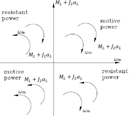
In this paper it is assumed that the transmission has two inertias: 𝐽1 on motor side

and 𝐽2 on load side. In Fig. 1.1, if 𝑀𝐿+ 𝐽2𝛼𝐿 and 𝜔𝑚 have the same sign, the load

introduces motive power to the motor; if they have opposite signs, the load introduces resistant power to the motor.

And the corresponding power flows are shown in Fig. 1.3 and Fig. 1.4. 𝑀_𝐿+ 𝐽₂𝛼_𝐿 Motor Transmission 𝐽₁ 𝐽2 𝑀_𝐿+ 𝐽₂𝛼_𝐿 𝑀_𝐿+ 𝐽₂𝛼_𝐿 𝑀𝐿+ 𝐽2𝛼𝐿 𝑀_𝐿+ 𝐽₂𝛼_𝐿

(12)

Fig. 1.3Direct power flow

Fig. 1.4 Inverse power flow

In Fig. 1.3 and Fig. 1.4 the power flow loss due to the direct and inverse efficiency is shown. In order to choose a brushless motor, apart from transmission ratio, we should take into account both direct and inverse efficiencies. In the second and fourth quadrant, the efficiency is direct, while in the first and third quadrant, the efficiency is inverse. That is, when 𝑀𝐿 and 𝜔𝐿 have the same sign, the efficiency is

direct; but when they have opposite signs, the efficiency is inverse.

In this paper, we will apply a new mathematic method to find out the right motor for a specific load.

In chapter 2, some basic knowledge, which will be very useful, are introduced, such as brushless motor, harmonic drive transmission, conic section.

𝑀_𝑚𝜔_𝑚 _𝑀 𝐿𝜔𝐿 (1 − 𝜂𝑑) 𝑀𝑚− (𝐽𝑀 + 𝐽1)𝛼𝑚 𝜔𝑚 J₁α_𝑀ω_m 𝐽𝑀𝛼𝑚𝜔𝑚 𝐽1𝛼𝑚𝜔𝑚 𝐽2𝛼𝐿𝜔𝐿 𝑀_𝐿𝜔_𝐿 𝑀_𝑚𝜔_𝑚 𝐽_𝑀𝛼_𝑚𝜔_𝑚 _𝐽 2𝛼𝐿𝜔𝐿 (1 − 𝜂_𝑖)(𝑀_𝐿+ 𝐽₂𝛼_𝐿)𝜔_𝐿 𝐽₁𝛼_𝑚𝜔_𝑚

(13)

In chapter 5, this method is applied to dynamic operating range.

In chapter 6, a simple example which applies this method to choose the appropriate transmission and motor is presented.

(14)

Chapter 2: Brushless Motor

Chapter 2: Drive system

characterization

2.1 AC Brushless Motor

2.1.1 Construction of a AC brushless motor

The brushless motor here is assembled with permanent magnets, and it is an electric motor driven by an alternating current. The brushless motors are based on magnetic rotating field.

A brushless motor having permanent magnets that can be used as a prime mover for automobiles, in place of internal combustion engines, since the motor can yield high torque during low speed rotation, as in the case of conventional types of brushless motors and can be used at high torque and with excellent motor efficiency at rotations three times as high as that of conventional types.

The brushless motor having permanent magnets according to the invention comprises a stator having a plurality of stator magnetic poles and a winding for generating a rotating field in the stator magnetic poles, a rotor having a rotating shaft and field permanent magnets rotating with respect to the stator magnetic poles ,a control circuit for detecting the position of magnetic poles of the field permanent magnet with respect to the stator and feeding current to the winding in accordance with the position; where in the field permanent magnets comprise a first field

permanent magnet having magnetic poles of different polarities alternately arranged in the direction of rotation, and a second field permanent magnet that is adapted to be rotatable with respect to the first field permanent magnet and has magnetic poles of different polarities alternately arranged in the direction of rotation; the first and second field permanent magnets facing the stator magnetic poles, and a mechanism for changing the phase of the synthesized magnetic poles of the first and second field permanent magnets in accordance with the rotation of the rotor is provided.(see Fig.

(15)

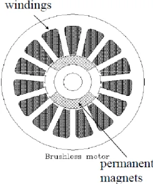
Fig. 2.1 An overall construction of a AC brushless motor

Fig. 2.1 shows the section structure of a brushless motor. We can see that the

windings are in the stator. The permanent magnets are in the rotor. A position

transducer allows us to know the position Ɵ𝑚 of the rotor, i.e. of the magnetic field.

(16)

2.1.2 Alternating Current (AC) Motor

There is no brush or sliding contact in the AC brushless motors. Heat is generated in the stator winding and the thermal resistance, to transmit heat to the environment, is very small. So they have advantages compared to the DC motors:

 Higher current limit due to the commutator contact.  Higher maximum speed than DC machine

 Light rotor and consequently low inertia. The brushless motor has great response quickness.

 High power and torque density.

 Less maintenance problem and sparkling problems due to no commutator. The AC motors are based on magnetic rotating field.

2.1.3 The basic electro-magnet

The magnetic permeability of an iron cylinder (diameter 𝐷, length 𝑙) is much larger than that of the air; an N turn winding is placed on diametrical plane; a constant current 𝐼𝑒 flows into the winding. This device acts like a permanent magnet with

cylindrical shape. The north pole is the surface from which the magnetic field lines come out, and the south pole is the surface in which the magnetic field lines enter (shown in Fig. 2.3).

(17)

Fig. 2.4 A hollow cylinder (stator)

2.1.4 Electro-magnetic joint: the alignment law

Fig. 2.5 Electro-magnetic joint

In Fig. 2.5, if the two basic permanent-magnets or electromagnets are put one inside the other, an aligning torque arises.

The torque depends on the value of the angle as a sine function: 𝑇 = −𝐾 𝑠𝑖𝑛 𝜀. And the torque acts so as to align the opposite magnetic polarities.

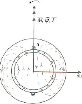
From joint to motor, if the magnetic polarities of the external magnet could rotate around the cylinder axis, this would make the alignment torque drag the inner permanent magnet thus providing a rotation. The rotation of the polarities of the external magnets can be achieved by using an external three-phase winding and placing a permanent magnet on the rotor. And the magnetic field produced by magnets or electro-magnets of cylindrical shape can be represented by vector oriented in the direction of the field line. As shown in Fig. 2.6, the vectors are called space phasors, and 𝑀𝑒, 𝑀𝑖 are the magneto motive force space phasors of external

(18)

Fig. 2.6 Electro-magnetic joint in motor

2.1.5 The three-phase windings

Three windings a, b and c are displaced by 120° one from each other; three ideal current generators feed the windings with balanced AC three-phase currents 𝑖𝑎, 𝑖𝑏

and 𝑖𝑐; the resulting magnetic field is the sum of the field produced by the single

windings. Then a rotating magnetic field is obtained (shown in Fig. 2.7).

(19)

𝑓 =3

2𝑁𝐼𝑀∙ 𝑒𝑗𝜔𝑡 (2.1)

Also the balanced three-phase current system can be represented by a rotating current space phasor 𝐼 , and the three-phase flux linkage can represented by a rotating space phasor 𝛹 too (see Fig. 2.8 ).

Fig. 2.8 Representation of space phasors

Then we know that the voltage can be represented by a space phasor, after project the rotating space phasor on each phase axes we can obtain the instantaneous value of phase variable(shown in Fig. 2.9), and the expressions are:

{ 𝑣𝑎 = 𝑅𝑎𝑖𝑎+𝑑𝛹_𝑑𝑡𝑎 𝑣𝑏 = 𝑅𝑏𝑖𝑏+𝑑𝛹_𝑑𝑡𝑏 𝑣_𝑐 = 𝑅_𝑐𝑖_𝑐+𝑑𝛹𝑐 𝑑𝑡 𝑣𝑠 = 𝑅𝑠𝑖𝑠+ 𝑑𝛹𝑠 𝑑𝑡 (2.2)

(20)

Fig. 2.9 The voltage space phasor

The flux and current are related by a constant: the synchronous (self) inductance 𝐿𝑠 ,

and we have:

𝛹 = 𝐿_𝑠𝑖_𝑠 (2.3)

(21)

As shown in Fig. 2.10, the stator rotating field (produced by the three-phase stator windings) produces an aligning torque that interacts with the rotor permanent magnet field, and the two fields run synchronously, i.e. the rotor’s angular speed is equal to the stator’s rotating field.

As we mentioned in 2.1.6, the voltages depend on the total flux 𝛹𝑠 produced by the

stator (rotating field) and by the rotor’s permanent magnet. Then we project the space phasors on a fixed axes reference frame α-β or on a synchronous rotating frame d-q, that is:

{

𝑣𝑠𝑠 = 𝑣𝑠𝑒𝑖𝜔𝑡

𝑖_𝑠𝑠 = 𝑖_𝑠𝑒𝑖𝜔𝑡

𝛹𝑠𝑠 = 𝛹𝑠𝑒𝑖𝜔𝑡

(2.4)

A rotating reference frame d-q is chosen having axes that are synchronous with the rotor’s permanent magnet flux space phasor 𝛹𝑠,

𝛹𝑠𝑠 = 𝛹𝑠∙ 𝑒𝑗𝜔 (2.5)

Where 𝛹𝑠 = 𝛹𝑚+ 𝐿𝑠𝑖𝑠, and it’s the total flux referred to a fixed reference frame α-β;

𝛹𝑠𝑠 is the total flux referred to a rotating reference frame d-q(shown in Fig. 2.11).

(22)

Chapter 2: Brushless Motor The total flux vector (referred to a fixed frame α-β) is:

𝛹𝑠𝑠 = 𝛹𝑚𝑠+ 𝐿𝑠𝑖𝑠𝑠 (2.6)

The total flux vector (referred to a rotating frame d-q) is: 𝛹_𝑠𝑒𝑖𝜔𝑡 _{= 𝛹}

𝑚𝑒𝑖𝜔𝑡+ 𝐿𝑠𝑖𝑠𝑒𝑖𝜔𝑡 (2.7)

Taking the total time derivative: 𝑑𝛹𝑠𝑒𝑖𝜔𝑡 𝑑𝑡 = 𝑖𝜔𝛹𝑚𝑒𝑖𝜔𝑡+ 𝐿𝑠 𝑑𝑖𝑠 𝑑𝑡 𝑒𝑖𝜔𝑡+ 𝑖𝜔𝐿𝑠𝑖𝑠𝑒𝑖𝜔𝑡 (2.8) Thus 𝑣_𝑠𝑒𝑖𝜔𝑡_{= 𝑅} 𝑠𝑖𝑠𝑒𝑖𝜔𝑡+ 𝑑𝛹𝑠 𝑑𝑡 𝑒𝑖𝜔𝑡= (𝑅𝑠𝑖𝑠+ 𝑖𝜔𝛹𝑚+ 𝐿𝑠 𝑑𝑖𝑠 𝑑𝑡 + 𝑖𝜔𝐿𝑠𝑖𝑠) 𝑒𝑖𝜔𝑡 (2.9) Simplifying the 𝑒𝑖𝜔𝑡 term we obtain:

𝑣_𝑠 = 𝑅_𝑠𝑖_𝑠+ 𝑖𝜔𝛹_𝑚+ 𝐿_𝑠𝑑𝑖𝑠

𝑑𝑡 + 𝑖𝜔𝐿𝑠𝑖𝑠 (2.10)

Then it is possible to project the vectors along the reference axes d (real) and q (imaginary):

𝛹𝑚 = 𝛹𝑚 (2.11)

𝑖_𝑠 = 𝑖_𝑠𝑑+ 𝑖 ∙ 𝑖_𝑠𝑞 (2.12)

The following two-axis model is therefore obtained: { 𝑣𝑠𝑑 = 𝑅𝑠𝑖𝑠𝑑 + 𝐿𝑠 𝑑𝑖_𝑠𝑑 𝑑𝑡 − 𝜔𝐿𝑠𝑖𝑠𝑞 𝑣𝑠𝑞 = 𝑅𝑠𝑖𝑠𝑞+ 𝐿𝑠 𝑑𝑖𝑠𝑞 𝑑𝑡 + 𝜔(𝐿𝑠𝑖𝑠𝑑 + 𝛹𝑚) (2.13)

Because the driving torque 𝑀𝑚 can be obtained from an energy balance, the

mechanical equation has to be considered to complete the model:

𝐽𝜔̇ = 𝑀_𝑚− 𝑀_𝐿 (2.14)

The power entering the motor is equal to:

W = 𝑣𝑠∗ 𝑖𝑠 = 𝑣𝑠𝑑𝑖𝑠𝑑+ 𝑣𝑠𝑞𝑖𝑠𝑞 (2.15)

(23)

In Eq. (2.16) we can see that the power entering the motor is made up of three parts: The power loses in the windings 𝑅𝑠(𝑖𝑠𝑑2+ 𝑖𝑠𝑞2); the power of magnetic energy

variation 𝐿𝑠(𝑑𝑖_𝑑𝑡𝑠𝑑𝑖𝑠𝑑+𝑑𝑖_𝑑𝑡𝑠𝑞𝑖𝑠𝑞) and the mechanical power exiting the motor

𝜔𝛹_𝑚𝑖_𝑠𝑞. The mechanical power exiting the motor is therefore equal to:

𝑊𝑚 = 𝑀𝑚∙ 𝜔 = 𝜔𝛹𝑚𝑖𝑠𝑞 (2.17)

Thus, the electro-magnetic torque is:

𝑀_𝑚 = 𝛹_𝑚𝑖_𝑠𝑞 (2.18)

If windings with N pole pairs are used, the rotor angular speed 𝜔𝑚 is different from

the current frequency 𝜔𝑒𝑙 by a factor 𝑁. Also the torque varies (increases) by a

factor 𝑁: 𝜔𝑚 = 𝜔_𝑒𝑙 𝑁 = 𝜔 𝑁 (2.19) 𝑀_𝑚 = 𝑁𝛹_𝑚𝑖_𝑠𝑞 (2.20)

So the complete model is:

{ 𝑣𝑠𝑑 = 𝑅𝑠𝑖𝑠𝑑 + 𝐿𝑠 𝑑𝑖𝑠𝑑 𝑑𝑡 − 𝜔𝐿𝑠𝑖𝑠𝑞 𝑣_𝑠𝑞 = 𝑅_𝑠𝑖_𝑠𝑞+ 𝐿_𝑠𝑑𝑖𝑠𝑞 𝑑𝑡 + 𝜔(𝐿𝑠𝑖𝑠𝑑+ 𝛹𝑚) 𝐽𝜔_𝑚̇ = 𝐽𝜔̇ 𝑁 = 𝑁𝛹𝑚𝑖𝑠𝑞− 𝑀𝐿 (2.21)

2.1.8 The working range of AC brushless motor

The working range of a brushless motor can reach higher speeds and torques and is nearly rectangular.

(24)

Fig. 2.12 Working range of brushless motor

As shown in the Fig. 2.12 the working range can be approximately subdivided into a continuous working zone (delimited by the motor rated torque 𝑀𝑀,𝑆1) and a

dynamic zone (delimited by the maximum motor torque 𝑀𝑀,𝑑𝑦𝑛). Usually the motor

rated torque decreases slowly with the motor speed 𝜔𝑚. In this paper, it is

considered constant and equal to 𝑀𝑀,𝑆1.

The nominal motor torque 𝑀𝑀,𝑟𝑎𝑡𝑒𝑑 is usually specified by the manufacturer in the

catalogues. The 𝑀𝑀,𝑆1 is defined as the torque that can be supplied by the motor

for an infinite time without overheating. The trend of maximum torque of the dynamic working range 𝑀𝑀,𝑑𝑦𝑛 is very complex. Because of the sparkles in the

commutator it will go down when the speed is very high near the 𝜔𝑀,𝑚𝑎𝑥. The trend

of 𝑀𝑀,𝑑𝑦𝑛 also depends on many other factors and it is difficult to express it with an

equation. So in this paper we assume it is constant and equal to 𝑀𝑀,𝑑𝑦𝑛.

Here we discuss the constraints of the brushless motor. 𝑀_{𝑀,𝑑𝑦𝑛}

𝑀

𝑀𝑀,𝑟𝑎𝑡𝑒𝑑

𝑀_𝑀,𝑆1

(25)

The root mean square torque generates the same energetic dissipation which is actually present in the cycle.

𝑀_{𝑚,𝑟𝑚𝑠}(𝜔) = √1 𝑇∫ 𝑀𝑚 2_{(𝑡)𝑑𝑡} 𝑇 0 (2.22)

In the operation the maximum torque 𝑀𝑚,𝑚𝑎𝑥 is:

𝑀_{𝑚,𝑚𝑎𝑥} = 𝑚𝑎𝑥 |𝑀_𝑚(𝑡)| Where 0 ≤ 𝑡 ≤ 𝑇 (2.23) The following set is the condition that must be satisfied by the motor:

{

𝑀_{𝑚,𝑚𝑎𝑥} ≤ 𝑀_{𝑀,𝑑𝑦𝑛} 𝑀_{𝑚,𝑟𝑚𝑠} ≤ 𝑀_𝑀,𝑆1 𝜔𝑚,𝑚𝑎𝑥 ≤ 𝜔𝑀,𝑚𝑎𝑥

(2.24)

Because 𝑀𝑚,𝑟𝑚𝑠 and 𝑀𝑚,𝑚𝑎𝑥 are univocal functions of 𝐽𝑀. Therefore we can plot

the corresponding 𝑀𝑚,𝑟𝑚𝑠 and 𝑀𝑚,𝑚𝑎𝑥 diagrams.

2.2 Transmission

The mechanical power is the product of a torque for a speed. Generally speaking, it is easier to produce mechanical power with small torques at high speeds; the

transmission performs the task of changing the distribution of power, adjusting the optimal conditions for tis production to the ones for its optimum use. This work done by the transmission usually involves reducing speed while increasing the available torque.

The transmission depends on the transmission ratio 𝜏 and on the transmission efficiency 𝜂 and the inertia 𝐽𝑇. if the transmission is an ideal one, the efficiency 𝜂

would be 1 and the inertia 𝐽𝑇 equals to 0.

A realistic model of the transmission has to consider the inevitable loss of power. The power dissipated affects the resulting performance of the machine and the choosing of correct motor.

It is defined that the transmission ratio 𝜏 : 𝜏 =𝜔𝑜𝑢𝑡

𝜔_𝑖𝑛 (2.25)

The relationship between the input acceleration and the output is shown below: 𝛼_𝑖𝑛 = 𝜔_𝑖𝑛̇ =𝜔𝑜𝑢𝑡̇

𝜏 =

𝛼𝑜𝑢𝑡

𝜏 (2.26)

(26)

Chapter 2: Brushless Motor 𝜂 =𝑃𝑜𝑢𝑡 𝑃𝑖𝑛 = 𝑀𝑜𝑢𝑡 𝑀𝑖𝑛 𝜔𝑜𝑢𝑡 𝜔𝑖𝑛 = 𝑀𝑜𝑢𝑡 𝑀𝑖𝑛 𝜏 ≤ 1

Where the 𝑀𝑜𝑢𝑡 and 𝑀𝑖𝑛 represent output and input torque of the transmission

and the 𝜔𝑜𝑢𝑡and the 𝜔𝑖𝑛 are the corresponding angular speeds.

In a more realistic model, i.e. at the situation: 𝜂 ≠ 1 as shown in Eq. (2.27) and Eq. (2.28), the power flow is sometimes from the motor to the load which is said to work with direct power flow, otherwise from the load to the motor which is said to work with inverse power flow. The transmission power losses are described by two different mechanical efficiency values 𝜂𝑖 and 𝜂𝑑.

𝜂_𝑑 = 𝑃𝑜𝑢𝑡,𝐿

𝑃_{𝑖𝑛,𝑚} (Direct power flow)(2.27) 𝜂_𝑖 = 𝑃𝑜𝑢𝑡,𝑚

𝑃_{𝑖𝑛,𝐿} (Inverse power flow)(2.28) In Eq. (2.27), the symbol 𝑃𝑖𝑛,𝑚 represents the power generated by motor flowing

into the transmission and 𝑃𝑜𝑢𝑡,𝐿 represents the power flowing out from the

transmission into the load.

Similarly, in Eq. (2.28), the symbol 𝑃𝑖𝑛,𝐿 represents the power generated by the load

flowing into the transmission and 𝑃𝑜𝑢𝑡,𝑚 represents the power flowing out from the

(27)

2.3 Conic sections

Fig. 2.13 Conic sections

The conic sections (shown in Fig. 2.13) are the no degenerate curves generated by the intersections of a plane with one or two nappes of a cone. For a plane

perpendicular to the axis of the cone, a circle is produced. For a plane that is not perpendicular to the axis and that intersects only a single nappe, the curve produced is either an ellipse or a parabola.

The curve produced by a plane intersecting both nappes is a hyperbola. The ellipse and hyperbola are known as central conics.

In the Cartesian coordinate system, the graph of a quadratic equation in two variables is always a conic section – though it may be degenerate, and all conic sections arise in this way. The equation will be of the form:

𝑎₁₁𝑥2_{+ 2𝑎}

12𝑥𝑦 + 𝑎22𝑦2+ 2𝑎13𝑥 + 2𝑎23𝑦 + 𝑎33 = 0 (2.29)

In Eq. (2.29) 𝑎11, 𝑎12, 𝑎22 are not all zero.

The above equation can be written in matrix notation as 𝑥 𝑦 ∙ [𝑎_𝑎11 𝑎12

12 𝑎22] ∙ [

𝑥

𝑦] + 2𝑎13𝑥 + 2𝑎23𝑦 + 𝑎33= 0

(28)

𝛿 = 𝑑𝑒𝑡 ([𝑎_𝑎11 𝑎12

12 𝑎22]) = −𝑎22 2_{+ 𝑎}

11𝑎12

If the conic is non-degenerate, then we have below conditions: 1. If 𝛿 > 0, the equation represents an ellipse;

 If 𝑎11= 𝑎22 and 𝑎12= 0, the equation represents a circle, which is a

special case of an ellipse;

2. If 𝛿 = 0, the equation represents a parabola; 3. If 𝛿 < 0, the equation represents a hyperbola;

 If we also have 𝑎11+ 𝑎22= 0, the equation represents a rectangular

(29)

Chapter 3: Method to solve direct and inverse efficiencies

Chapter 3: Method to solve direct and

inverse efficiencies

In the following section, we will take into consideration the use of the method which can solve both direct and inverse efficiencies and the transmission inertia.

3.1 Mathematical model of a machine

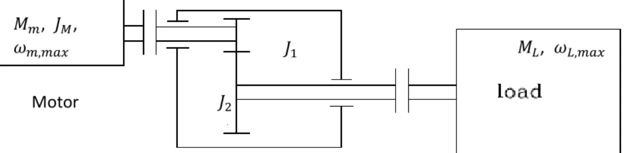
Fig. 3.1 A generic machine considered inertia in transmission

A generic machine is shown in the Fig. 3.1. It is assumed that the moment of inertia of transmission has two parts: 𝐽1 and 𝐽2. On the left side a motor is connected to

the gear in the transmission which has the moment of inertia 𝐽1, while on the right

side the load is connected to the gear in the transmission whose inertia is 𝐽2

In the transmission from motor point of view, we can get the equation of power balance:

1

2𝐽2′𝜔𝐿2 = 1

2𝐽2𝜔𝑀2 (3.1) Then, bearing in mind Eq. (2.25), we can obtain ω𝑀 =ω_𝜏𝐿, so combining with Eq.

(3.1), we obtain

𝐽2′ = 𝐽2𝜏2

So the total inertia of transmission is:

𝐽_𝑇 = 𝐽₁+ 𝐽₂′ _{= 𝐽}

1 + 𝐽2𝜏2 (3.2)

The inertia of the transmission is known. The acceleration law α𝐿(t) is designed

according to the task motion we need. 𝐽₂

𝐽₁ 𝑀𝐿, 𝜔𝐿,𝑚𝑎𝑥

𝑀𝑚, 𝐽𝑀,

𝜔𝑚,𝑚𝑎𝑥

(30)

We know there are direct and inverse power flows. In general, the power flows and their relations with the efficiencies are very complex. In this paper we assume that the power flow is sometimes direct and sometimes inverse.

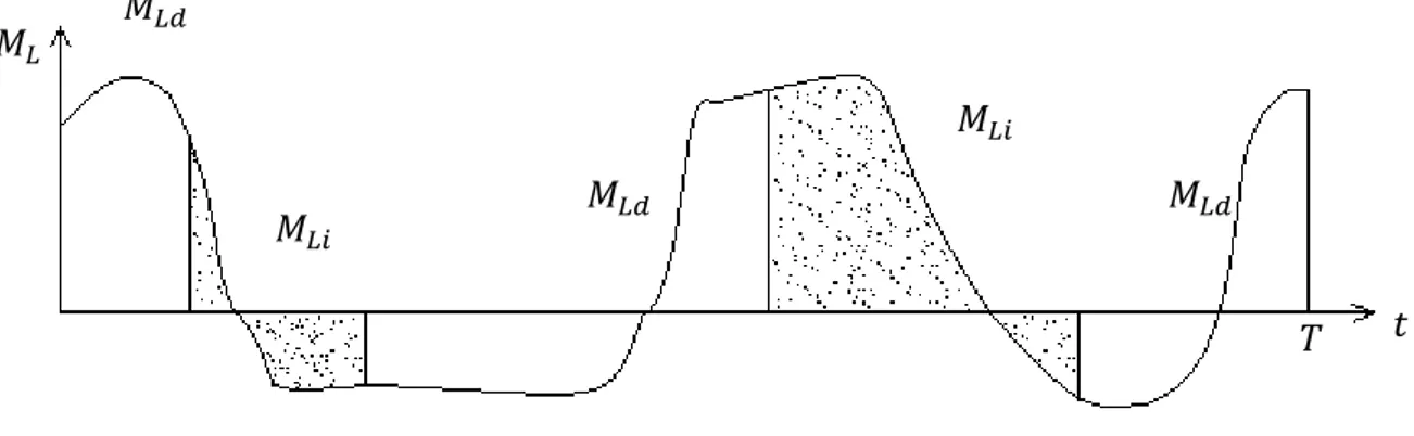
Fig. 3.2 ML-time curve

As shown in Fig. 3.2, the ML-time curve is divided into 2 curves (shown in Fig. 3.3 and Fig. 3.4): 𝑀𝐿𝑑 which means the torque produces a direct power flow; while the

other one is 𝑀𝐿𝑖 represent the torque for inverse power flow.

We can easily achieve the inequality from the Fig. 1.2:

{

(𝑀𝐿+𝐽2 𝛼𝐿)𝜔𝐿 > 0 𝑑𝑖𝑟𝑒𝑐𝑡 𝑒𝑓𝑓𝑖𝑐𝑖𝑒𝑛𝑐𝑦

(𝑀_𝐿+𝐽₂𝛼_𝐿)𝜔_𝐿 = 0 (𝑀𝐿+𝐽2 𝛼𝐿)𝜔𝐿 < 0 𝑖𝑛𝑣𝑒𝑟𝑠𝑒 𝑒𝑓𝑓𝑖𝑐𝑖𝑒𝑛𝑐𝑦

(3.3)

If (𝑀𝐿+𝐽2𝛼𝐿)𝜔𝐿 > 0, the load torque has the same rotating direction with the

angular speed. Find the time domain of this zone; let the 𝑀𝐿𝑑 to represent the

torque of direct efficiency. The system has the direct efficiency.

Similarly, if (𝑀𝐿+𝐽2 𝛼𝐿)𝜔𝐿 < 0, the load torque has the opposite rotating direction

with respect to the angular speed. So the system has the inverse efficiency. Let the 𝑀_𝐿𝑖 to represent the torque of inverse efficiency.

However, the situation when (𝑀𝐿+𝐽2 𝛼𝐿)𝜔𝐿 = 0 is a little complex. It is assumed

that the motor works periodically. The time 𝑇 is the cycle time. Here two possibilities come:

If the angular speed is not zero, i.e. 𝜔𝐿 ≠ 0, it is obvious that (𝑀𝐿+ 𝐽2 𝛼𝐿) = 0.

𝑀_𝐿 𝑡 𝑇 𝑀𝐿𝑑 𝑀_𝐿𝑖 𝑀𝐿𝑑 𝑀𝐿𝑑 𝑀_𝐿𝑖

(31)

If at the initial time of the motion (𝑡 = 0) the situation is (𝑀𝐿+𝐽2𝛼𝐿)𝜔𝐿 = 0 and

𝜔_𝐿 = 0. The system will has the same power flow efficiency as the situation at the end of the period. For example, for 𝑡 = 𝑇, the system has direct efficiency, the system will have the direct efficiency at 𝑡 = 0 when (𝑀𝐿+𝐽2 𝛼𝐿)𝜔𝐿 = 0.

After the analysis, the ML-time curve will be split into two curves: MLd-time curve and MLi-time curve, so we can obtain the direct and inverse components separately, and

it is very convenient for further research.

Fig. 3.3 MLd-time curve

Fig. 3.4 MLi-time curve

In this paper we assume the transmission is already known: 𝐽1, 𝐽2, 𝜏, 𝜂𝑑 and 𝜂𝑖.

Due to the transmission efficiency, the inertia of transmission will have some changes. The following shows the equilibriums from the motor point of view.

When the system has direct transmission efficiency, from the Fig. 1.3 and Eq. (2.27) we can have the equation of the power balance:

𝜂𝑑𝑃𝑖𝑛,𝑚= 𝑃𝑜𝑢𝑡,𝐿 (3.4)

From the Fig. 1.3, we can easily find out the 𝑃𝑖𝑛,𝑚 in Eq. (3.4) represents the input

power flow coming from the motor on the left side of the transmission which includes three parts: the positive power produced by the motor, the negative power loss due to the inertia 𝐽𝑀 of the motor and the negative power loss due to the

inertia 𝐽1 of the transmission.

t T MLd t T MLi

(32)

𝑃_{𝑖𝑛,𝑚}= 𝑀_𝑚𝜔_𝑚− 𝐽_𝑀𝛼_𝑚𝜔_𝑚− 𝐽₁𝛼_𝑚𝜔_𝑚 (3.5) And 𝑃𝑜𝑢𝑡,𝐿 in Eq. (3.4) represents the output power flow on the right side of the

transmission which includes two parts: the positive power loss due to the inertia 𝐽2

of the transmission and the final output power to the load.

𝑃_{𝑜𝑢𝑡,𝐿} = 𝑀_𝐿𝜔_𝐿+ 𝐽₂𝛼_𝐿𝜔_𝐿 (3.6) Use these two equations to substitute in Eq. (3.4), we can obtain:

𝜂_𝑑 𝑀_𝑚𝜔_𝑚− (𝐽_𝑀+ 𝐽₁)𝛼_𝑚𝜔_𝑚 = (𝑀_𝐿+ 𝐽₂𝛼_𝐿)𝜔_𝐿 (3.7) Remembering in mind Eq. (2.26), we achieve the relation between the acceleration of motor and the load:

𝛼_𝑚 = 𝛼𝐿

𝜏 (3.8)

We replace Eq. (3.8) in Eq. (3.7):

𝜂_𝑑[𝑀_𝑚− (𝐽_𝑀+ 𝐽₁)𝛼𝐿

𝜏] 𝜔𝑚 = (𝑀𝐿+ 𝐽2𝛼𝐿)𝜔𝐿 (3.9) Dividing all the terms in Eq. (3.9) by 𝜏, we obtain

𝑀𝑚 𝜏 = 𝐽𝑀 𝜏2𝛼𝐿+ 𝐽1 𝜏2𝛼𝐿+ 𝐽2 𝜂𝑑𝛼𝐿+ 𝑀𝐿 𝜂𝑑 (3.10)

Then, combining the inertia parts of transmission, we obtain 𝑀_𝑚 𝜏 = 𝐽_𝑀 𝜏2𝛼𝐿+ ( 𝐽₁ 𝜏2+ 𝐽₂ 𝜂_𝑑)𝛼𝐿+ 𝑀_𝐿 𝜂_𝑑 (3.11) We indicate by 𝐽𝑇,𝑑: 𝐽𝑇,𝑑 = 𝐽₁ 𝜏2+ 𝐽₂ 𝜂𝑑 (3.12)

Similarly, when the system has direct transmission efficiency, from the Fig. 1.4 and Eq. (2.28) we can have the equation of the power balance:

𝜂𝑖𝑃𝑖𝑛,𝐿 = 𝑃𝑜𝑢𝑡,𝑚 (3.13)

From the Fig. 1.4, we can easily find out the 𝑃𝑖𝑛,𝐿 in Eq. (3.13) represents the input

power flow coming from the load on the right side of the transmission which includes two parts: the power generated by the load and inertia 𝐽2 of the

(33)

Chapter 3: Method to solve direct and inverse efficiencies the motor.

𝑃𝑜𝑢𝑡,𝑚 = 𝑀𝑚𝜔𝑚− 𝐽1𝛼𝑚𝜔𝑚− 𝐽𝑀𝛼𝑚𝜔𝑚 (3.15)

Substitute them in Eq. (3.13), we can achieve:

𝜂_𝑖(𝑀𝐿+𝐽2𝛼𝐿)𝜔𝐿 = [𝑀𝑚− (𝐽𝑀+ 𝐽1)

𝛼𝐿

𝜏] 𝜔𝑚 (3.16)

By dividing by 𝜏 and leaving 𝑀_𝜏𝑚 to the first member we obtain 𝑀𝑚 𝜏 = 𝐽𝑀 𝜏2𝛼𝐿+ 𝐽1 𝜏2𝛼𝐿+ 𝜂𝑖𝐽2𝛼𝐿+ 𝑀𝐿𝜂𝑖 𝑀𝑚 𝜏 = 𝐽𝑀 𝜏2𝛼𝐿+ ( 𝐽1 𝜏2+ 𝜂𝑖𝐽2)𝛼𝐿+ 𝑀𝐿𝜂𝑖 (3.17) We indicate by 𝐽𝑇,𝑖: 𝐽𝑇,𝑖= 𝐽₁ 𝜏2+ 𝜂𝑖𝐽2 (3.18) It is easy to get: 𝑀𝑚 = 𝐽_𝑚 𝜏 𝛼𝐿+ 𝜏 (𝐽𝑇,𝑑𝛼𝐿+ 𝑀_𝐿 𝜂𝑑) (3.19) 𝑀_𝑚 =𝐽𝑚 𝜏 𝛼𝐿+ 𝜏(𝐽𝑇,𝑖𝛼𝐿+ 𝜂𝑖𝑀𝐿) (3.20) In order to simplify them, we introduce 𝑀𝐿∗

𝑀_𝐿∗ _{= {}𝐽𝑇,𝑑𝛼𝐿+ 𝑀𝐿 𝜂𝑑 𝑖𝑓 (𝑀𝐿+ 𝐽2𝛼𝐿) > 0 𝐽𝑇,𝑖𝛼𝐿+ 𝜂𝑖𝑀𝐿 𝑖𝑓 (𝑀𝐿+ 𝐽2𝛼𝐿) < 0 (3.21) So we obtain 𝑀𝑚 = 𝐽𝑚 𝜏 𝛼𝐿+ 𝜏𝑀𝐿∗ (3.22)

(34)

Chapter 4: Apply the method to continuous duty operating range

Chapter 4: Apply the method to

continuous duty operating

range

In this chapter, we will introduce a method to deal with the continuous duty working range of the motor.

4.1 Introduction to the MM,s1 and τth

𝑀_𝑀,𝑆1 depends on the thermal characteristics of the motor. The motor warms up because of:

 Joule effect (copper losses);

 Parasitic currents and Hysteresis (iron losses);  Mechanical losses (bearings, etc.).

The motor can suffer a maximum internal temperature Ɵ𝑀,𝑚𝑎𝑥, above which the

sheathing “burns”. Let us consider 𝑀𝑚 and 𝜔𝑚constant, which indicates that the

motor is in mechanical steady state. And then the wasted power 𝑊𝑤 in the motor is

constant.

However, it is possible that the motor is not at thermal steady state. After a thermal transient, the motor tends to reach a steady state temperature Ɵ𝑀,𝑚𝑎𝑥. If

Ɵ𝑚,𝑚𝑎𝑥 ≤ Ɵ𝑀,𝑚𝑎𝑥 , the motor reaches Ɵ𝑚,𝑚𝑎𝑥. On the contrary, if Ɵ𝑚,𝑚𝑎𝑥 >

(35)

Fig. 4.1 Temperature profile versus time

The nominal torque 𝑀𝑀,𝑆1 corresponds to the limit condition: Ɵ𝑚,𝑚𝑎𝑥 = Ɵ𝑀,𝑚𝑎𝑥.

Therefore, the nominal torque MM,S1 is the maximum torque that the motor can

exert without burning in mechanical and thermal steady state. So the constraint inequality is |𝑀𝑚𝑜| ≤ 𝑀𝑀,𝑆1.

Then we introduce 𝜏𝑡ℎ, which is the thermal time constant of the motor.

If the mechanical behavior of the motor is periodic (with period T), we can make a good approximation if the following three conditions are satisfied:

1) 𝑇 ≪ 𝜏𝑡ℎ: in this condition the motor warming up depends on the average wasted

power 𝑊̅𝑊 in the period, and not on the instantaneous power (which varies

significantly in the period);

2) The motor torque is proportional to the current:

𝑀_𝑚 = 𝐾_𝑇𝑖 (4.1)

3) The motor wasted power 𝑊𝑤 is only due to the Joule Effect:

𝑊𝑤 = 𝑅𝑖2 (4.2)

Then bearing in mind Eq. (2.22), and the average wasted power is 𝑊̅_𝑊= 𝐸𝑊 𝑇 = 1 𝑇∫ 𝑊𝑊(𝑡) 𝑑𝑡 = 1 𝑇∫ 𝑅𝑖2 (𝑡) 𝑇 0 𝑑𝑡 = 𝑅1 𝑇∫ 𝑀𝑚2(𝑡) 𝐾_𝑇2 𝑑𝑡 𝑇 0 𝑇 0 = 𝑅 𝐾𝑇2 1 𝑇∫ 𝑀𝑚2(𝑡) 𝑑𝑡 = 𝑅 𝐾𝑇2 𝑀_{𝑚,𝑟𝑚𝑠}2 𝑇 0 (4.3)

(36)

4.2 The JM versus Mm,rms curve

By applying Eq.(3.22), now the root mean square of the torque due to both direct and inverse efficiencies can be expressed as:

𝑀𝑚,𝑟𝑚𝑠2 = 1 𝑇∫ 𝑀𝑚2𝑑𝑡 = 𝑇 0 1 𝑇∫ ( 𝐽_𝑚2 𝜏2 + 𝜏2𝑀𝐿∗2+ 2𝐽𝑚𝛼𝐿𝑀𝐿∗) 𝑇 0 𝑑𝑡 = {1 𝑇∫ 𝐽_𝑚2 𝜏2 𝛼𝐿2𝑑𝑡 + 1 𝑇∫ 𝜏2𝑀𝐿∗2𝑑𝑡 + 1 𝑇∫ 2𝐽𝑚𝛼𝐿𝑀𝐿∗𝑑𝑡 𝑇 0 𝑇 0 𝑇 0 } =𝐽𝑚 2 𝜏2 𝛼𝐿,𝑟𝑚𝑠2+ 𝜏2𝑀𝐿,𝑟𝑚𝑠∗ 2_{+ 2𝐽} 𝑚𝐺𝐿 (4.4) Where 𝐺𝐿 = 1 𝑇∫ 𝛼𝐿𝑀𝐿∗𝑑𝑡 𝑇 0

And 𝛼𝐿,𝑟𝑚𝑠 and 𝑀𝐿,𝑟𝑚𝑠∗ are the root mean square of the angular acceleration and

the generalized load.

𝛼_{𝐿,𝑟𝑚𝑠} = √1 𝑇∫ 𝛼𝐿2𝑑𝑡 𝑇 0 𝑀_{𝐿,𝑟𝑚𝑠}∗ _{= √}1 𝑇∫ 𝑀𝐿∗2𝑑𝑡 𝑇 0

In the previous studies, the transmission is an unknown factor while the motors are known. The old method is from motor point of view to choose the transmission. However in this case all the parameters of transmission are known, which means the transmission ratio 𝜏 and the transmission inertia 𝐽1,𝐽2 are known. Now we choose

motor from transmission point of view.

For this situation, it is reasonable to draw the JM -Mm,rms curve and to check if the

motor satisfies the curve conditions. Each motor has the parameters of Mm,rms and JM.

It is easy to plot the motor on the curve using the point (𝐽𝑀 , 𝑀𝑚,𝑟𝑎𝑡𝑒𝑑). Each point

(37)

Chapter 4: Apply the method to continuous duty operating range After having simplified:

𝑀𝑚,𝑟𝑚𝑠= √𝐴𝐽𝑀2+ 2𝐵𝐽𝑀 + 𝐶 (4.6) Where 𝐴 =𝛼𝐿,𝑟𝑚𝑠 2 𝜏2 = 1 𝜏2 1 𝑇∫ 𝛼𝐿2𝑑𝑡 𝑇 0 (4.7) 𝐵 = 𝐺_𝐿 = 1 𝑇∫ 𝛼𝐿𝑀𝐿∗𝑑𝑡 𝑇 0 (4.8) 𝐶 = 𝜏2_𝑀 𝐿,𝑟𝑚𝑠∗ 2 = 𝜏2 1 𝑇∫ 𝑀𝐿∗2𝑑𝑡 𝑇 0 (4.9)

Now let us discuss Eq. (4.6). From the formulas (4.7) and (4.9), we can know that: 𝐴 ≥ 0 𝑎𝑛𝑑 𝐶 ≥ 0

And if 𝐴 = 0 then 𝐵 = 0, because

𝐴 =𝛼𝐿,𝑟𝑚𝑠2

𝜏2 = 0

So 𝛼𝐿,𝑟𝑚𝑠 = √1_𝑇∫ 𝛼₀𝑇 𝐿2𝑑𝑡= 0

Then 𝛼𝐿(𝑡) = 0 ∀𝑡.

Then bearing in mind Eq. (4.8), we can prove that 𝐵 = 0.

In order to have a better analysis of Eq. (4.6), a variable D is induced: D = 𝐵2_{− 𝐴𝐶}

It is possible to show that:

D = 𝐵2_{− 𝐴𝐶 ≤ 0}

To sum up, the system must satisfy these conditions: {𝐴 ≥ 0𝐶 ≥ 0

𝐷 ≤ 0 If 𝐴 = 0, 𝐵 = 0.

In fact, Eq. (4.6) is a conic section formula. We can rewrite it into the form: 𝑎11𝐽𝑀2+ 2𝑎12𝐽𝑀𝑀𝑚,𝑟𝑚𝑠+ 𝑎22𝑀𝑚,𝑟𝑚𝑠2+ 2𝑎13𝐽𝑀+ 2𝑎23𝑀𝑚,𝑟𝑚𝑠+ 𝑎33= 0

(38)

The matrix of the conic section is 𝑀 = [

𝑎₁₁ 𝑎₁₂ 𝑎₁₃ 𝑎₁₂ 𝑎₂₂ 𝑎₂₃ 𝑎₁₃ 𝑎₂₃ 𝑎₃₃] So Eq. (4.6) becomes: 𝐴𝐽_𝑀2− 𝑀_{𝑚,𝑟𝑚𝑠}2+ 2𝐵𝐽_𝑀+ 𝐶 = 0 (4.10) So 𝑀 = [𝐴0 −1 00 𝐵 𝐵 0 𝐶]

And the discriminant of the conic section is

𝛿 = 𝑑𝑒𝑡 ([𝐴 0

0 −1]) = −𝐴

From the formula it is known that:

If 𝐴 > 0 then the curve will be a hyperbola. If 𝐴 = 0 then it will become a parabola.

If 𝐶 = 0 then the curve will pass though the origin point.

If 𝐷 = 0 which means = ±√𝐴𝐶 , the curve will become two straight lines. 𝑀𝑚,𝑟𝑚𝑠= √𝐴𝐽𝑚2± 2√𝐴𝐶𝐽𝑚+ 𝐶

= √(√𝐴𝐽𝑚± √𝐶) 2

=√𝐴𝐽𝑚± √𝐶 (4.11)

(39)

1. If 𝐴 > 0, 𝐶 > 0, 𝐵 > 0 and 𝐷 < 0 then the JM -Mm,rms curve is as below:

Fig. 4.2 JM -Mm,rms curve

As the figure shown above, Eq. (4.10) is a hyperbola curve. The orange part of the curve shows the real JM -Mm,rms curve because both JM and Mm,rms must be greater

than zero. And the directrix of the curve is always at the line 𝐽𝑀 = −𝐵_𝐴, which is on

the left of the ordinate, so in this case, the minimum 𝑀𝑚,𝑟𝑚𝑠 is useless. And the

minimum 𝑀𝑚,𝑟𝑚𝑠 of the orange curve is bigger, and it is √𝐶, at the abscissa 𝐽𝑀 = 0.

And the orange part is ascending.

−𝐵

𝐴

𝐽_𝑀 𝑀𝑚,𝑟𝑚𝑠

(40)

2. If 𝐴 > 0, 𝐶 > 0, 𝐵 = 0 and 𝐷 < 0 then the JM -Mm,rms curve is like below:

As the figure shows above, Eq. (4.10) is also a hyperbola curve. The directrix of the curve is at the abscissa 𝐽𝑀 = 0 because

−𝐵

𝐴 = 0

The minimum 𝑀𝑚,𝑟𝑚𝑠 is at where 𝐽𝑀 = −𝐵_𝐴 = 0, so in this case, the orange part

that we need contains the real minimum 𝑀𝑚,𝑟𝑚𝑠. And the orange part is ascending.

−𝐵

𝐴 𝐽𝑀

(41)

3. If 𝐴 > 0, 𝐶 > 0, 𝐵 < 0 and 𝐷 < 0 then the JM -Mm,rms curve is like below:

As Fig. 4.4 shows above, Eq. (4.10) is a hyperbola curve. The directrix of the curve lies on right side of 𝐽𝑀 = 0 because 𝐽𝑀 = −𝐵_𝐴> 0, so the directrix is on the right of the

ordinate axis, and minimum 𝑀𝑚,𝑟𝑚𝑠is at the abscissa 𝐽𝑀 = −𝐵_𝐴, and is useful,

because it’s also the minimum point of the orange part that we need. And we can also see that the orange curve descends before 𝐽𝑀 = −𝐵_𝐴, and then ascends after

𝐽_𝑀 = −𝐵_𝐴.

4. If 𝐴 > 0, 𝐷 = 0, 𝐵 > 0 .

Because we have D = 𝐵2− 𝐴𝐶 = 0, Eq. (4.10) becomes two straight lines. 𝐵2 _{= 𝐴𝐶}

And then:

𝐶 =𝐵

2

𝐴 > 0 Then, the JM -Mm,rms curve is as below:

−𝐵

𝐴

𝐽_𝑀 𝑀_{𝑚,𝑟𝑚𝑠}

(42)

The directrix of the curve lies on left side of the ordinate axis, because 𝐽𝑀 = −𝐵_𝐴 < 0.

And the orange JM -Mm,rms curve becomes a straight line, and its minimum point is

not at the abscissa 𝐽𝑀 = −𝐵_𝐴, but at the abscissa 𝐽𝑀 = 0. So the orange part is

ascending.

5. If 𝐴 > 0, 𝐷 = 0, 𝐵 = 0

Because we have D = 𝐵2− 𝐴𝐶 = 0, Eq. (4.10) becomes two straight lines. From 𝐵2 = 𝐴𝐶 = 0 then

𝐶 = 0 Then, the JM -Mm,rms curve is shown in Fig. 4.6:

−𝐵

𝐴

(43)

As the figure shows, Eq. (4.10) becomes two straight lines which pass through the origin point (0, 0), which is also the minimum point. The directrix of the curve is at 𝐽𝑀 = 0 because B = 0. The orange real JM -Mm,rms curve becomes a line which start

from the origin point. And the orange part is ascending.

6. If 𝐴 > 0, 𝐷 = 0, 𝐵 < 0

As before because D = 𝐵2− 𝐴𝐶 = 0, Eq. (4.10) becomes two straight lines 𝐵2 _{= 𝐴𝐶 > 0}

And then:

𝐶 =𝐵2 𝐴 > 0 The JM -Mm,rms curve is as below in Fig. 4.7:

−𝐵

𝐴 𝑀𝑚,𝑟𝑚𝑠

(44)

As the figure shows, Eq. (4.10) also consists of two straight lines due to D = 𝐵2_{− 𝐴𝐶 = 0. The directrix of the curve lies on the right side of ordinate,}

because 𝐽𝑀 = −𝐵_𝐴 > 0. The orange real JM -Mm,rms curve becomes a polyline, which

descends before 𝐽𝑀 = −𝐵_𝐴, and then ascends after 𝐽𝑀 = −𝐵_𝐴.

−𝐵

𝐴

(45)

7. If 𝐴 = 0, 𝐷 = 0, 𝐵 = 0 and 𝐶 > 0 then the JM -Mm,rms curve is as below in Fig. 4.8:

As the figure shows, Eq. (4.10) becomes two parallel straight lines. In fact the formula becomes:

𝑀𝑚,𝑟𝑚𝑠2 = 𝐶

When 𝐶 > 0

𝑀𝑚,𝑟𝑚𝑠 = ±√𝐶

So the curves are two parallel lines. But we only care about the line which is in the first quadrant, which is the orange part shown in Fig. 4.7.

𝑀_{𝑚,𝑟𝑚𝑠}

(46)

Chapter 4: Apply the method to continuous duty operating range We use these JM -Mm,rms curves to choose the motor.

As shown in Fig. 4.9, a point 𝑅 ≡ (𝐽𝑀, 𝑀𝑚,𝑟𝑎𝑡𝑒𝑑) represents a motor, where

𝑀_{𝑚,𝑟𝑎𝑡𝑒𝑑} is the rated torque of a motor. If the point is above the curve 𝑠 shown in the figure, the motor satisfies the condition:

𝑀𝑚,𝑟𝑚𝑠≤ 𝑀𝑚,𝑟𝑎𝑡𝑒𝑑 𝑀𝑚,𝑟𝑎𝑡𝑒𝑑 𝐽_𝑀 𝑀_{𝑚,𝑟𝑚𝑠} 𝐽_𝑀 0 s 𝑅

(47)

Chapter 5: Apply the method to dynamic operating range

Chapter 5: Apply the method to

dynamic operating range

5.1 Dependence of Mm on JM in a given instant

[1]

𝑀_{𝑀,𝑑𝑦𝑛} depends on the electronic converter driving the motor. The converter transistors can suffer a maximum peak current without burning for a small time range. Because of the proportionality between 𝑀𝑚 and 𝑖, the torque 𝑀𝑀,𝑑𝑦𝑛

corresponds to this current.

From previous analysis, we know that in order to let the motor become feasible it must satisfy three conditions, i.e. it does not only satisfy 𝑀𝑚,𝑟𝑚𝑠 ≤ 𝑀𝑀,𝑆1 and

𝜔𝑚,𝑚𝑎𝑥 ≤ 𝜔𝑀,𝑚𝑎𝑥, but also

𝑀_{𝑚,𝑚𝑎𝑥} ≤ 𝑀_{𝑀,𝑑𝑦𝑛}

So it is necessary to check if the maximum torque of the motor during the cycle is smaller than the maximum torque the motor can provide.

In order to obtain the 𝐽𝑀-𝑀𝑚,𝑚𝑎𝑥 curve we need to adopt a different approach,

which, apart from achieving the same results, allows us to focus attention on the most exacting condition for the system. We know according to the machine design and the definition of the reference task, during the system working there are lots of pairs of angular accelerations and the generalized torques of the load like (α𝐿, 𝑀𝐿∗).

Therefore we wish to identify them in the reference task, which are directly responsible for the limitations in the motor maximum torque, i.e. 𝑀𝑚,𝑚𝑎𝑥.

For a given instant 𝑡, we consider about the pair (α𝐿, 𝑀𝐿∗). In the same instant 𝑡, we

take into account Eq. (3.22) written in the form where 𝑀𝑚 is a function of 𝐽𝑀, and

expressed in Eq.(5.4)

𝑀_𝑚 = 𝐽𝑀

𝜏 α𝐿+ 𝑀𝐿∗𝜏 = α𝐿

𝜏 𝐽𝑀+ 𝑀𝐿∗𝜏 (5.1) In fact the pair (α𝐿, 𝑀𝐿∗) is time consumed, which means α𝐿(t) and 𝑀𝐿∗(𝑡) are

functions of time. Considering the plane (α𝐿, 𝑀𝐿∗), it is advisable to use a diagram

that presents α𝐿 in abscissa and 𝑀𝐿∗ in ordinate. Once α𝐿(t) and 𝑀𝐿∗(𝑡) are

known, because the transmission ratio 𝜏 is given, 𝑀𝑚 is a linear function of 𝐽𝑀. In

fact, the inertia of the motor is always positive. So 𝐽𝑀 satisfies the condition:

(48)

During a time period, it is possible to use the discrete points to show the angular accelerations and the generalized torques of the load. As Fig. 5.1 shown below, the discrete points represent the pairs of (α𝐿, 𝑀𝐿∗).

Fig. 5.1 The discrete points of αL –ML*

Since the transmission ratio 𝜏 and the pair (α𝐿, 𝑀𝐿∗) are known, Eq. (5.1) will

become several straight lines that use 𝐽𝑀 as the abscissa and 𝑀𝑚 as ordinate. Each

pair of angular acceleration and generalized torque forms a linear function. The slope of the line is α_𝜏𝐿 and the point of intersection between the graph of the function and the 𝑀𝑚-axis is 𝑀𝐿∗𝜏 .

We now consider the J𝑀 versus 𝑀𝑚 curves. There are four cases.

1. α𝐿 ≥ 0 and 𝑀𝐿∗ ≥ 0

In this case, in the plane 𝛼𝐿-𝑀𝐿∗ the corresponding point 𝑆 lies in the first quadrant.

From Eq. (5.1) we can know that both the slope 𝛼_𝜏𝐿 and the 𝑀𝑚-intercept are

positive. In the 𝐽𝑀-𝑀𝑚 plane we obtain a corresponding curve

𝑠 lying in the first quadrant because 𝐽𝑀 is positive (shown in Fig. 5.2).

In fact, because of 𝐽𝑀 > 0, the curve 𝑠 has a minimum point (0, 𝑀𝐿∗𝜏).

𝑀_𝐿∗

(49)

Fig. 5.2 Curve s in plane JM-Mm when αL>0 and ML*>0

If α𝐿 = 0 then the curve 𝑠 will become a horizontal line which parallels to the

abscissa JM, passing the point (0, 𝑀𝐿∗𝜏).

If 𝑀_𝐿∗ = 0 then the curve 𝑠 remains a linear function with the slope 𝛼_𝜏𝐿, passing through the origin point (0, 0).

If α𝐿 = 0 and 𝑀𝐿∗ = 0 then the curve 𝑠 will overlap the abscissa 𝐽𝑀.

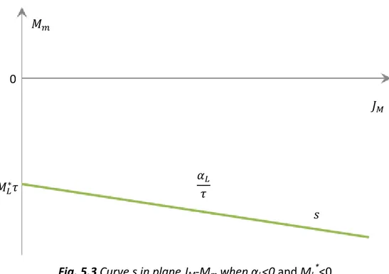
2. α𝐿 ≤ 0 and 𝑀𝐿∗ ≤ 0

In this case, in the plane 𝛼𝐿-𝑀𝐿∗ the corresponding point 𝑆 lies in the third

quadrant. From Eq. (5.1) we can know that both the slope α_𝜏𝐿 and the 𝑀𝑚-intercept

are negative. In the plane 𝐽𝑀-𝑀𝑚 we obtain a corresponding curve 𝑠 lying in the

fourth quadrant due to JM is always positive (shown in Fig. 5.3).

𝐽_𝑀 𝑀_𝑚 𝑀_𝐿∗_𝜏 𝛼_𝐿 𝜏 𝑠 0

(50)

Fig. 5.3 Curve s in plane JM-Mm when αL<0 and ML*<0

Obviously this curve is symmetric of the curve corresponding to the coordinates (|𝛼𝐿|, |𝑀𝐿∗|) which respect to the abscissa axis.

3. α𝐿 < 0 and 𝑀𝐿∗ > 0

In this case, in the plane 𝛼𝐿-𝑀𝐿∗ the corresponding point 𝑆 lies in the second

quadrant. From Eq. (5.1) we can know that the slope 𝛼_𝜏𝐿 is negative, and the 𝑀_𝑚-intercept is positive. In the plane 𝐽𝑀-𝑀𝑚 we obtain a corresponding curve 𝑠

lying in the first quadrant and in the fourth quadrant (shown in Fig. 5.4). 𝑀_𝑚 𝐽𝑀 𝑀_𝐿∗_𝜏 0 𝛼𝐿 𝜏 𝑠

(51)

Fig. 5.4 Curve s in plane JM-Mm when αL<0 and ML*>0

The curve 𝑠 is monotonically descending and it is easy to solve the intersection point between the curve and the abscissa 𝐽𝑀. According to Eq. (5.1):

𝑀𝑚 = α_𝐿 𝜏 𝐽𝑀+ 𝑀𝐿∗𝜏 = 0 So we can get: 𝐽_𝑀 = −𝑀𝐿 ∗_𝜏2 α_𝐿 (5.2)

The formula indicates the curve 𝑠 passing through the point (−𝑀_α𝐿∗𝜏2

𝐿 , 0). In this

case, the inertial torque of the motor is used for balancing the load, while the motor does not exert any torque Mm.

Furthermore, both α𝐿 and 𝑀𝐿∗ vary over time, so that the point 𝑆 changes in the

second quadrant of the plane 𝛼𝐿-𝑀𝐿∗. The corresponding curve 𝑠 and its

intersection with the abscissa axis in the plane 𝐽𝑀-𝑀𝑚 also vary.

4. α𝐿 > 0 and 𝑀𝐿∗ < 0

In this case, in the plane 𝛼𝐿-𝑀𝐿∗ the corresponding point 𝑆 lies in the fourth

quadrant. From Eq. (5.1) we can know that the slope α_𝜏𝐿 is positive, and the 𝑀_𝑚-intercept is negative. In the plane 𝐽𝑀-𝑀𝑚 we obtain a corresponding curve 𝑠

lying in the first quadrant and in the fourth quadrant (shown in Fig. 5.5).

Obviously, this curve is symmetric of the curve corresponding to the coordinates (−|α_𝐿|, |𝑀_𝐿∗_{|) with respect to the abscissa axis.}

𝑀_𝑚 𝐽_𝑀 𝑀_𝐿∗_𝜏 0 𝑀_𝐿∗_𝜏2 α𝐿 𝑠

(52)

Fig. 5.5 Curve s in plane JM-Mm when αL>0 and ML*<0

Obviously, both α𝐿 and 𝑀𝐿∗ vary over time, so that the point S changes in the

second quadrant of the plane 𝛼𝐿-𝑀𝐿∗. The corresponding curve 𝑠 and its

intersection with the abscissa axis in the plane 𝐽𝑀-𝑀𝑚 also vary.

5. |𝑀𝑚| versus 𝐽𝑀

In Fig. 5.6 there are some curves representing the absolute value |𝑀𝑚| versus 𝐽𝑀

with different values of α𝐿 and 𝑀𝐿∗. From Eq. (5.1) we obtain

|𝑀𝑚| = | 𝛼𝐿 𝜏 𝐽𝑀+ 𝑀𝐿∗𝜏| (5.3) 𝑀_𝑚 𝐽𝑀 𝑀_𝐿∗_𝜏 0 𝑀_𝐿∗_𝜏2 α_𝐿 𝑠 𝑀_𝑚 𝛼_𝐿𝑀_𝐿∗ _{< 0} 𝛼_𝐿𝑀_𝐿∗ _{> 0}

(53)

If 𝛼𝐿 > 0 and 𝑀𝐿∗ > 0, the curve in Fig. 5.6 remains unaffected with respect to that

in Fig. 5.2.

If 𝛼𝐿 < 0 and 𝑀𝐿∗ < 0, the curve in Fig. 5.6 is symmetric of that in Fig. 5.3 with

respect to the abscissa axis.

If α𝐿 < 0 and 𝑀𝐿∗ > 0, as the Fig. 5.6 shows, the curve does not lie in the first and

in the fourth quadrant, but rather only in the first one. |𝑀𝑚| has a minimum value,

which is an edge point, on the abscissa 𝐽𝑀 = −𝑀𝐿

∗_𝜏2

α𝐿 with an ordinate equal to 0. On

the left of the minimum point the curve descends monotonically. This branch is equal to the corresponding branch in Fig. 5.4, while on the right of the minimum point the curve ascends monotonically when 𝐽𝑀 increases. This branch is symmetric of the

corresponding branch in Fig. 5.4 with respect to the abscissa axis.

If α𝐿 > 0 and 𝑀𝐿∗ < 0, as the Fig. 5.6 shows, the curve no longer lies in the first

and in the fourth quadrant, but rather only in the first one. |𝑀𝑚| has a minimum

value, which is an edge point, on the abscissa 𝐽𝑀 = −𝑀𝐿

∗_𝜏2

α𝐿 with an ordinate equal to

0. On the left of the minimum point the curve descends monotonically when 𝐽𝑀

increases. This branch is symmetric of the corresponding branch in Fig. 5.5 with respect to the abscissa axis, while on the right of the minimum point the curve ascends monotonically when 𝐽𝑀 increases. This branch is equal to the

corresponding branch in Fig. 5.5.

In any case, the curve |𝑀𝑚| versus 𝐽𝑀 is continuous.

5.2 The Mm,max

versus J

M curve[1]

We wish to find the maximum torque among the linear lines of 𝐽𝑀-𝑀𝑚. The curve

𝑀𝑚,𝑚𝑎𝑥 versus JM depends on 𝛼𝐿 and 𝑀𝐿∗, both of which assume different values

over time. For each value of 𝐽𝑀, our aim is to obtain the maximum value assumed

over time by 𝑀𝑚. In presence of many pairs (α𝐿, 𝑀𝐿∗), we now consider, for each

value of 𝐽𝑀, ,the curve having the maximum value of 𝑀𝑚. Therefore we obtain a

new curve, which is the curve JM-Mm,max. The calculation of Mm,max can be expressed:

𝑀_{𝑚,𝑚𝑎𝑥} = 𝑚𝑎𝑥

𝐽𝑀 |𝑀𝑚| = 𝑚𝑎𝑥𝑡 [|

𝛼𝐿(𝑡)

𝜏 𝐽𝑀 + 𝑀𝐿∗(𝑡)𝜏|] (5.4) We can now start by considering only two curves s and t, corresponding to two

generic points 𝑆 ≡ (𝛼𝐿,𝑆, 𝑀𝐿,𝑆∗ ) and 𝑇 ≡ (𝛼𝐿,𝑇, 𝑀𝐿,𝑇∗ ). These curves are shown in Fig.

(54)

Fig. 5.7 Example of JM-Mm,max curve corresponding to two pairs of values (αL,S, ML,S*) and (αL,T, ML,T*)

We intend to show the 𝐽𝑀-𝑀𝑚,𝑚𝑎𝑥 curve is continuous, and has only one the

minimum value of 𝑀𝑚,𝑚𝑎𝑥.

It is possible to think that in some abscissas ranges the curve 𝑠 lies above the curve 𝑡 and the 𝐽𝑀- 𝑀𝑚,𝑚𝑎𝑥 curve 𝑙 coincides with the corresponding continuous

branches of 𝑠. On the contrary, in other abscissas ranges the curve 𝑡 lies above the curve 𝑠 and the curve 𝑙 coincides with the corresponding continuous branches of 𝑡. The transition from a branch of s to a branch t happens with continuity in the intersection points between s and t, just as Fig. 5.7 shows. Because of the reasons mentioned above, the 𝐽𝑀-𝑀𝑚,𝑚𝑎𝑥 curve is continuous.

Now let us discuss the minimum value of the curve 𝑙. There are three main cases of the 𝐽𝑀-𝑀𝑚,𝑚𝑎𝑥 curve

5.2.1 The two pairs of value (α

L,S

, M

L,S

*) and (α

L,T

, M

L,T

*) in the first or

third quadrant:

𝑅𝑡 𝐽𝑀 𝑀𝑚,𝑚𝑎𝑥 𝑠 𝑡 𝑙 𝑅 𝑅_𝑠

(55)

5.2.1.1 |αL,S |< |αL,T |and | ML,S*|<| ML,T*|

Fig. 5.8 Example of JM-Mm,max curve corresponding to two pairs of values (αL,S, ML,S*) and (αL,T, ML,T*)

As Fig. 5.8 shows above, the curve 𝑠 and t have no intersection points. And the minimum point of one curve (for example, curve 𝑡 in Fig. 5.8) lies above the other curve (curve 𝑠 in Fig. 5.8), then the minimum point 𝑅𝑡 of the curve 𝑡 is a

minimum point of the 𝐽𝑀-𝑀𝑚,𝑚𝑎𝑥 curve 𝑙. In fact, since the curve 𝑡 is above curve

𝑠, the curve 𝑙 is overlapping the whole curve 𝑡. Because of this reason, the minimum point of curve 𝑙 coincides with the curve 𝑡, which means 𝑅𝑡 ≡ 𝑅.

We can also consider the plane αL versus 𝑀𝐿∗ to analyze the relative position of the

two points 𝑆𝑠 ≡ (|𝛼𝐿,𝑆|, |𝑀𝐿,𝑆∗ |) and 𝑆𝑡 ≡ (|𝛼𝐿,𝑇|, |𝑀𝐿,𝑇∗ |). It is obvious that 𝑆𝑠 lies

on the left side of 𝑆𝑡 which means that the curve 𝑠 does not give contribution to

the curve 𝑙.

Therefore in this situation, the point 𝑅𝑡 is the only minimum point of the curve 𝑙.

5.2.1.2 |𝜶𝑳,𝑺| < |𝜶𝑳,𝑻| and |𝑴𝑳,𝑺∗ | > |𝑴𝑳,𝑻∗ |

In this case, as Fig. 5.9 shows, the curve 𝑠 and 𝑡 have one intersection point. Because both slopes are greater than zero, the two curves are monotonically ascending. 𝑅_𝑡 ≡ 𝑅 𝑅𝑠 _𝐽_𝑀 𝑀_{𝑚,𝑚𝑎𝑥} 𝑠 𝑡 𝑙 0