Climatological analysis of temperature and salinity fields in the Mediterranean sea

(1)

Alma Mater Studiorum · Universit`

a di Bologna

Scuola di Scienze

Corso di Laurea Magistrale in Fisica

Climatological analysis of temperature and

salinity fields in the Mediterranean Sea

Relatore:

Prof. Nadia Pinardi

Correlatore:

Dott. Simona Simoncelli

Correlatore:

Dott. Marina Tonani

Presentata da:

Michela Giusti

Sessione II

(2)

Acknowledgements

I am very grateful to my supervisor Professor Nadia Pinardi for his invaluable guidance and constant encouragement throughout my work and in the preparation of this thesis. Many thanks are also due to Dr. Simona Simoncelli, Dr. Marina Tonani and Alessandro Grandi for their thoughtful advice, precious help and cooperation.

Special thanks go to my parents, Luigina and Franco, and my aunt Antonietta for their unfailing encouragement and trust, as well as their support, both material and immaterial, throughout my studies, and, last but not least, to my ﬁancée, Giacomo, for his inﬁnite patience, wisdom, and caring attitude. To him I dedicate this thesis.

(3)

(4)

Abstract

A climatological field is a mean gridded field that represents the monthly or seasonal trend of an ocean parameter. This instrument allows to understand the physical conditions and physical processes of the ocean water and their impact on the world climate. To construct a climatolog-ical field, it is necessary to perform a climatologclimatolog-ical analysis on an historclimatolog-ical dataset. In this dissertation, we have constructed the temperature and salinity fields on the Mediterranean Sea using the SeaDataNet 2 dataset. The dataset contains about 140000 CTD, bottles, XBT and MBT profiles, covering the period from 1900 to 2013.

The temperature and salinity climatological ﬁelds are produced by the DIVA software using a Variational Inverse Method and a Finite Element numerical technique to interpolate data on a regular grid. Our results are also compared with a previous version of climatological ﬁelds and the goodness of our climatologies is assessed, according to the goodness criteria suggested by Murphy (1993). Finally the temperature and salinity seasonal cycle for the Mediterranean Sea is described.

Una climatologia rappresenta il campo medio mensile o stagionale di un parametro dell’oceano su una griglia regolare. Questo strumento permette di capire i processi e le condizioni ﬁsiche dell’acqua e il loro impatto sul clima. Per costruire una climatologia è necessario compiere un’analisi climatologica su un dataset storico. In questa tesi sono state create climatologie di temperatura e salinità del Mediterraneo usando il dataset SeaDataNet 2. Questo dataset comprende circa 140000 proﬁli misurati con CTD, bottiglie, XBT and MBT nel Mediterraneo e copre un periodo che va dal 1900 al 2013.

Per produrre le climatologie è stato usato il software DIVA che utilizza il Variational Inverse Method e il Finite Element method per interpolare i dati su una griglia regolare. Abbiamo poi comparato i risultati con quelli di una versione precedente, valutando la bontà delle nostre cli-matologie, in base ai criteri di ‘goodness’ introdotti da Murphy (1993). Inﬁne abbiamo descritto il seasonal cycle per la temperatura e la salinità nel Mediterraneo.

(5)

(6)

List of Figures

1.1 Mediterranean Sea. . . 3

1.2 Mediterranean Sea circulation at 15 m. . . 5

1.3 Mediterranean Sea circulation at 200–300 m. . . 6

1.4 Salinity ﬁeld at 10 m of the Mediterranean Sea. . . 8

1.5 Salinity ﬁeld at 10 m depth during November reconstructed from the statistical OA scheme. . . 8

1.6 Salinity ﬁeld at 10 m depth during November reconstructed from the variational inverse method. . . 9

1.7 MEDAR/MEDATLAS partners. . . 10

1.8 Example of salinity ﬁeld of MEDAR/MEDATLAS data set. . . 10

1.9 Prototype ATLAS moorings. . . 11

1.10 An ARGO proﬁling ﬂoat. . . 13

1.11 A proﬁling ﬂoat system. . . 13

1.12 A Niskin bottle. . . 13

1.13 A rosette. . . 13

1.14 An MBT. . . 15

1.15 An XBT. . . 15

(9)

1.17 A glider. . . 16

1.18 An example of a glider trajectory. . . 16

1.19 Altimetry satellite. . . 16

2.1 SeaDataNet partners. . . 18

2.2 SeaDataNet 2 Infrastructure. . . 19

2.3 SeaDataNet Common Data Index (CDI). . . 20

2.4 Work ﬂow diagram. . . 22

2.5 Numbers of proﬁles during years. . . 24

2.6 Percentages of types of instruments used from 1910 to 1987. . . 24

2.7 Percentages of types of instruments used from 1988 to 2013. . . 25

2.8 Month distribution. . . 26

2.9 Location of temperature and salinity proﬁles from 1910 to 2013. . . 27

2.12 Location of temperature proﬁles from 1910 to 2013. . . 28

2.13 Location of salinity proﬁles from 1910 to 2013. . . 29

2.14 Regions of the Mediterranean Sea. . . 29

2.15 Percentages of the total casts for each region. . . 30

2.16 Percentages of proﬁles for each region in the period 1910-1987. . . 31

2.17 Percentages of proﬁles for each region in the period 1988-2013. . . 31

2.18 Number of casts for seasons and regions from 1910 to 1987. . . 32

(10)

2.20 Western Mediterranean: Number of temperature measurements with respect to

depth. . . 34

2.21 Western Mediterranean: Number of salinity measurements with respect to depth. 35 2.22 Eastern Mediterranean: Number of temperature measurements with respect to depth. . . 35

2.23 Eastern Mediterranean: Number of salinity measurements with respect to depth. 36 2.24 Number of temperature measurements with respect to depth and season. . . 36

2.25 Number of salinity measurements with respect to depth and season. . . 37

2.26 Regions used for the Regional range test. . . 40

2.27 Quality Control ﬂag. . . 41

2.28 Example of map with wrong positions. . . 42

2.29 Map with land points. . . 42

2.30 Correct map. . . 43

2.31 Bathymetry of the Mediterranean Sea. . . 43

3.1 Example of interpolated proﬁle. . . 47

3.2 Gridding problem . . . 48

3.3 Diva example mesh. . . 51

4.1 Examples of monthly temperature and annual salinity background ﬁelds at dif-ferent depths for March. . . 55

4.2 Temperature climatologies of the surface for March, June, September, and De-cember. . . 58

4.3 Salinity climatologies of the surface divided by seasons. . . 59

4.4 Temperature climatologies at 100m for March, June, September, and December. 60 4.5 Salinity climatologies at 100 m divided by seasons. . . 61

(11)

4.6 Temperature climatologies at 500m for March, June, September, and December. 62

4.7 Salinity climatologies at 500 m divided by seasons. . . 63

4.8 Temperature error maps with the corresponding data distribution maps. . . 64

4.9 Salinity error maps with the corresponding data distribution maps. . . 65

4.10 Comparison of temperature climatologies V5 and V3 at the surface for (a)March, (b)June, (c)September and (d)December. . . 67

4.11 Comparison of salinity climatologies V5 and V3 at the surface divided by seasons ((a)Winter, (b)Spring, (c)Summer, (d)Autumn). . . 68

4.12 Comparison of temperature climatologies V5 and V3 at 100 m for (a)March, (b)June, (c)September and (d)December. . . 70

4.13 Comparison of salinity climatologies V5 and V3 at 100 m divided by seasons((a)Winter, (b)Spring, (c)Summer, (d)Autumn). . . 71

4.14 Comparison of temperature climatologies V5 and V3 at 500 m for (a)March, (b)June, (c)September and (d)December. . . 72

4.15 Comparison of salinity climatologies V5 and V3 at 500 m divided by seasons ((a)Winter, (b)Spring, (c)Summer, (d)Autumn). . . 73

4.16 V5 temperature monthly proﬁles of Standard Deviation. . . 75

4.17 V5 salinty monthly proﬁles of Standard Deviation. . . 75

4.18 V3 temperature monthly proﬁles of Standard Deviation. . . 76

4.19 V3 salinity monthly proﬁles of Standard Deviation. . . 76

4.20 Temperature RMSD percentages with respect to the V5 SD. . . 78

4.21 Salinity RMSD percentages with respect to the V5 SD. . . 78

4.22 Temperature MD percentages with respect to the V5 SD. . . 79

4.23 Salinity MD percentages with respect to the V5 SD. . . 79

(12)

4.25 Salinity RMSD percentages with respect to the V3 SD. . . 80

4.26 Temperature MD percentages with respect to the V3 SD. . . 81

4.27 Salinity MD percentages with respect to the V3 SD. . . 81

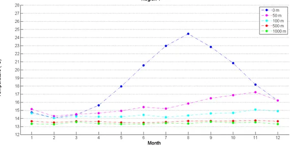
5.1 Temperature and salinity mean values of region 1. . . 84

5.14 Temperature means at surface in the Gulf of Maine as a function of calendar day. 97 5.15 Salinity means at surface in the Gulf of Maine as a function of calendar day. . . . 98

(13)

(14)

List of Tables

2.1 Data set institutes. . . 23

2.2 Data set casts divided for instrument. . . 24

2.3 Data set measurements. . . 25

2.4 Number of temperature and salinity proﬁles by seasons and regions from 1910 to 1987. . . 32

2.5 Hydrological casts divided for seasons and regions from 1988 to 2013. . . 33

2.6 Percentages of temperature measurements per interval of depth. . . 37

2.7 Percentages of salinity measurements per interval of depth. . . 37

2.8 Temperature, salinity, and depth Quality Flag values. . . 41

3.1 Statistical equivalence between the OA and VIM. . . 50

(15)

(16)

Chapter 1

Introduction

In physical oceanography, climatology is the study of the trend of a hydrological or biochemical propriety of the ocean for annual, seasonal, and monthly periods. These studies are important to understand the physical conditions and physical processes of the ocean water and their impact on the world climate. For this reason, the oceanographic community has been collecting a huge amount of experimental data for several decades, in order to create complete, multidisciplinary, and international data sets that allowed to construct climatological fields of the ocean param-eters. A climatological field is a mean field of an ocean parameter that represents the monthly or daily climatological state of the sea. This representation is ‘the smoothest field that respects the consistency with the observed values over the domain of interest’ [1] and permits to solve the ’gridding problem’: we can redistribute the parameter values from an irregular distribution to a regular grid.

The aim of this work is to produce new three-dimensional temperature and salinity ﬁelds in the Mediterranean Sea through climatological analysis of SeaDataNet 2 in situ data set.

The dissertation is organized as follows:

• In chapter 1, a brief history of the climatological analyses is outlined;

• In chapter 2, SeaDataNet 2 data set is described, including the eight principles of the quality control of the data set.

• In chapter 3, a description of the data analysis algorithms is performed.

(17)

• In chapter 5, a seasonal cycle analysis of temperature and salinity ﬁelds is performed.

• In chapter 6, the conclusions of the study are provided.

1.1 Climatological studies in the Mediterranean Sea

The Mediterranean Sea is among the oceanographically most interesting regions of the world ocean because of its unique features. Since many years, it has been the site of climatology projects. In fact, despite its little dimensions, it is the focus of a great range of processes and interactions, including for example, some physical processes of the global general circulation. The Mediterranean Sea is a semi-enclosed sea that has been divided by the oceanographers in two sub-basins: the Western Mediterranean and the Eastern Mediterranean. The boundary line between the two regions is the Sicily Strait. The reason for this division is not only geographic but especially related to hydrological and physical properties such as temperature, salinity, and circulation. As we can see from Figure 1.1, the Western Mediterranean includes: the Strait of Gibraltar, that controls the exchange of water between the Mediterranean Sea and the Atlantic Ocean; the Alboran Sea, enclosed between the Morocco coasts and the meridional Spain coasts; the Balearic Sea, which is delimited by the Spanish and French coasts in the West, and conﬁnes with the Algerian basin in the South, the Ligurian Sea in the North, and Sardinia and Corsica in the East; and the Tyrrhenian Sea, separated by the Sardinia channel. The Eastern Mediterranean includes the Adriatic Sea in the North, separated from the Southern Ionian basin by the Otranto strait, and the Levantine basin in the East, separated from the Aegean Sea by the Greek islands.

We now presents a brieﬂy description of the vertical structure of the Mediterranean water masses and the general circulation. Traditionally it is possible to identify three principal water masses, that are related to their formation locations:

• The Modiﬁed Atlantic Water (MAW), which is located between the surface and 100 m, entering from the Strait of Gibraltar. Its path proceed in the zonal direction and it is possible to follow it observing the salinity values between 20 (in the Western basin) to 50 m (in the eastern basin).

• The Levantine Intermediate Water (LIW), which is located between 200 and 300 m, is produced in the Levantine basin during winter. Its circulation goes from east to west.

(18)

F 1.1: Mediterranean Sea.

Source: http://media-2.web.britannica.com/eb-media/10/6010-004-373EBA60.jpg

• The Mediterranean Deep Water (MDW), which is the deep water mass, is separated in two reservoirs from the Strait of Sicily. The western part (WMDW) was produced during winter in the Gulf of Lions, the eastern part (EMDW) in the Adriatic and the Aegean Sea also in winter.

The Mediterranean general circulation is forced by the wind stress and the buoyancy fluxes. It is possible to notice from Figure 1.2 that the northern areas are characterized by cyclonic circulation while the souther areas by anticyclonic circulation. This is related to the wind stress curl sign. An important features present in the Mediterranean basin are the gyres that generally are forced by wind stress. The cyclonic gyres, presented in the northern areas, are forced also by deep and intermediate water formation, while the southern gyres are forced of the intermediate waters. Another important component of the Mediterranean Sea are the mesoscale eddies that are different from gyres for the persistency time. We start to describe the general surface circulation (see Figure 1.2) from the entering of the AW from Gibraltar, that meandering around the two Alboran gyres. These gyres are different in dimension and time persistence. Between the eastern Alboran gyre and a cyclonic eddy there is The Almera-Oran front that gives the name at the eddy: Almera-Oran cyclonic eddy. After the Almera-Oran front we can see two different currents: one going northward toward the Ibiza channel and the other forming

(19)

an important segment of the Algerian Current. In this zone there are a frequently growth of large anticyclonic eddies, persisting for several months. In the central western Mediterranean there is a eastward current called the Western MidMediterranean Current (WMMC). This current merges at north with the southern border of the cyclonic flow called the Gulf of Lion gyre that reachs a northward current also called the Liguro–Provenal–Catalan Current. Eastward of the Balearic Islands, the WMMC flows in the open ocean turning southward along the western coasts of Sardinia and forming an intensified current called the Southerly Sardinia Current (SSC). The SSC flows along the Tunisian coastlines and forms another segment of the Algerian Current in the Sardinia Channel. In the southern Tyrrhenian Sea the reformed Algerian Current is divided in three branches: two branches flows in the Strait of Sicily and the third flows in the Tyrrhenian Sea. Furthermore in the Tyrrhenian Sea we can find three cyclonic gyres: the South-Western Tyrrhenian Gyre (SWTG), the South-Eastern Tyrrhenian Gyre (SETG) and the Northern Tyrrhenian Gyre (NTG). The SWTG forms in the middle of the Tyrrhenian Sea a northward current, called the Middle Tyrrhenian Current (MTC). Through the Strait of Sicily, the Algerian Current branches into the Sicily Strait Tunisian Current (SSTC) along the southern coasts and the Atlantic Ionian Stream (AIS). At about 13◦E the SSTC turns northward around a large anticyclonic gyre called the Sirte Gyre (SG). The northern border of the SG is the AIS current that divided the Ionian Sea in two regions. North of the AIS there are an eastern boundary current, called Eastern Ionian Current (EIC), a weak cyclonic gyre, called the Northern Ionian Cyclonic Gyre and the Pelops Gyre (PG). Before passing the Cretan Passage the AIS forms a current along the North African coasts called the Cretan Passage Southern Current (CPSC). The other branches formed are the the Mid-Mediterranean Jet (MMJ) and the Southern Levantine Current (SLC). The first is located between the Mersa Matruh Gyre System (MMGS) at south and the Rhodes Gyre at north, and flows inside the Asia Minor Current that forms the Shikmona Gyre System. In the northern part of the Cretan Passage, before the Strait of Kassos, the continuation of the Asia Minor Current forms a large anticyclonic meander, encircling the area of the recurrent anticyclonic Ierapetra Gyre. The Adriatic Sea is dominated by the Middle and Southern Adriatic cyclonic gyres and the Eastern Adriatic Current and the Western Adriatic Coastal Current systems. The Aegean Sea shows a southward flow through the Cyclades (the Cretan Sea Westward Current (CSWC)) and in the northern area the circulation is dominated by a well-defined and high-intensity anticyclonic gyre: the North Aegean Sea Anticyclone (NASA).

(20)

F 1.2: Mediterranean Sea circulation at 15 m.

Source: Pinardi et al., 2013

the opposite direction to the surface circulation. The description starting from the Levantine basin because is the site of the LIW formation. The Rhodes Gyre and Ierapetra Ierapetra are consistent with the surface flow. The Mersa Matruh Gyre has a more varied structure due to a large meander of the MMJ and a large-amplitude anticyclone near the Egyptian coasts. The Shikmona Gyre System presents several anticyclonic semi–stationary eddies. the surface Cretan Sea Westward Current (CSWC) branches in the Ionian Sea into three streams at this depth. The first forms the southern border of the Pelops Gyre, the second turns eastward while the other joins the Sirte Gyre anticyclonic flow. The preferred path for the LIW is southward, along the Gulf of Sirte and westward LIW current of the Sicily Strait emerges as a branching of the SG south–western intensified current. Nortward of the AIS surface current there is a cyclonic gyre at this depth called the Northern Ionian Cyclonic Gyre (NICG). In the Western Mediterranean the LIW current turns cyclonically around the SWTG. The LIW path is characterized by two major branches one directed northward, toward the Gulf of Lion Gyre and the second westward toward the Strait of Gibraltar. At this depth the Gulf of Lion Gyre presents several cyclonic circulation structures inside the larger-scale gyre1_.

The Mediterranean Sea climatological water masses and the general circulation have been the object of study of many articles. One of the ﬁrst climatological analyses of hydrographic data as a basis of geostrophic circulation in the Mediterranean has been conducted by Ovchinnikov (1966) [2].

(21)

F 1.3: Mediterranean Sea circulation at 200–300 m.

Source: Pinardi et al., 2013

Subsequent attempts to improve the knowledge of properties and circulation in the Mediter-ranean Sea, in particular in the Eastern MediterMediter-ranean, brought ambiguous and contradictory results [3]. In 1982, on the occasion of a Congress of the International Commission for the Scien-tiﬁc Exploration of the Mediterranean, an international research group was formed, called POEM (Physical Oceanography of the Eastern Mediterranean, 1984), supported by IOC/UNESCO (the Integovermental Oceanographic Commission). The group focused on the description of the phe-nomenology of the Eastern Mediterranean, by both analysing historical data, and collecting new data. Moreover, the group modelled the circulation of the sea and its physical, biological and chemical fundamental processes. The focus on the Eastern Mediterranean Sea was motivated by the very scanty knowledge of this basin compared with other world regions [3] as well as by a special interest in some of its characteristics reproducing the global ocean general circulation but with multiple and interactive space and time scales [4].

Following the POEM effort, Hecth et al (1988) [5] succeeded in describing the climatological seasonal and instantaneous kinematical properties of the mesoscale flow field on the Levantine Basin through the climatological water masses properties and their seasonal variations. The authors used a long time series data that covered the period from February 1979 to August 1984 on a regular grid domain (a box of 2°30’ x 2° with the station located at 0.5°). They charac-terized some different water mass layers for temperature and salinity values and time duration. Furthermore they mapped the flow field and observed a new kind of mesoscale variabilities with the formation of eddies and jets never revealed before.

(22)

Climatological Atlas of World Ocean by Levitus (1982) [6]. Levitus used data of the National Oceanographic Data Center (NODC), Washington, D.C, that included temperature, salinity and oxygen data measured from stations, mechanical bathythermographs, and expendable bathyther-mographs of the previous eighty years. Levitus followed a standard procedure comprising a quality control and a statistical check to eliminate spurious data and an objective analysis at standard levels on a one degree latitude-longitude grid between the surface and ocean bottom with a maximum depth of 5500 m.

In Figure 1.4, we show a climatological salinity field of the Mediterranean Sea during winter, reconstructed with the Levitus atlas by Brasseur et al. (1996) (whose for a climatological work in the Mediterranean Sea, will be described further on). It can be noted that the general trends of this parameter were adequately represented ( in the Eastern Mediterranean values are higher than in the Western Mediterranean), although the spatial resolution did not conform to the regional scale. Levitus work was the start of the World Ocean Atlas (WOA) project by the Ocean Climate Laboratory of the National Oceanographic Data Center that produced new atlas at four year intervals from 1994 to 2013. The WOA project followed procedures that were similar to the ones employed by Levitus. In fact the WOA dataset consists of objectively-analysed global grids at 1° spatial resolution. Data are interpolated onto 33 standardised vertical intervals from the surface to 5500 m and the averaged fields are produced for annual, seasonal and monthly time-scales. The WOA 2013 extended the vertical levels from 33 to 102 to have more accurate quality control of observational data and study how mixed layer depth changes with reduced error. The WOA 2013 also added the 1° and 1/4° horizontal resolution versions for temperature and salinity field. All data and products are available on the WOA 2013 website2.

As far as the Western Mediterranean Sea is concerned, an important climatological study was performed by Picco (1990) [7] who reconstructed a numerical atlas from 15000 hydrographic proﬁles coming from diﬀerent sources for the period 1909-1987.

Brasseur et al. (1996)[1] introduced a new method to reconstruct the three dimensional ﬁelds of the properties of the Mediterranea Sea. Unlike their predecessors these authors used a variational inverse method to generate the climatological maps, rather than the objective analysis introduced by Gandin3 (1969). They also used the CTD data in addition to bottle data coming from several datasets covering the period 1900-1987, namely the BNDO (Bureau National del Données Océaniques, Brest,French) and the U.S. NODC. All those in situ data were collected in a single

2_{http://www.nodc.noaa.gov/OC5/woa13/}

(23)

F 1.4: Salinity ﬁeld at 10 m of the Mediterranean Sea.

Source: P. Brasseur et al. (1995)

dataset called MED2. After a brief description of the data distribution and reduction, Brasseur et al. concentrated on the variational analysis method to show that it was ‘mathematically equivalent but numerically more eﬃcient’ than the objective analysis. They in fact compared the results obtained with the objective analysis method (see Figure 1.5) with those obtained through the variational analysis method (see Figure 1.6): actually, only minimal diﬀerences can be noticed between the two maps.

F 1.5: Salinity ﬁeld at 10 m depth during November reconstructed from the statistical OA scheme.

With time, it has become evident that the results of such studies are inﬂuenced by the quantity and the quality of data used. Moreover new versions of those ﬁelds are an essential part of the

(24)

F 1.6: Salinity ﬁeld at 10 m depth during November reconstructed from the variational inverse method.

numerous toolkits used by oceanographers, engineers, managers, navies, and authorities to mon-itor the ocean state and variability, to infer possible climate changes, and to initialize models. This fostered the need of historical multidisciplinary archive of observational data which would be otherwise difficult to find, and could possibly be lost. The Intergovernmental Oceanographic Commission began to foster international projects to compile exhaustive data sets and make them available to the entire scientific community with a standard format and quality assurance procedure. After some important programmes such as GODAR4 _{(Global Oceanographic Data}

Archaeology and Rescue), and EU/MAST-MATER project [8] (Mass Transfer and Ecosystem Response ﬁnancially supported by the Marine Science and Technology programme of the Eu-ropean Unit), the most representative and comprehensive project for the Mediterranean and Black Sea was MEDAR/MEDATLAS II (Mediterranean Data Archaeology and Rescue) that collected historical data from about 1890 to 2002. SeaDataNet (2006-today) is the evolution of MEDAR/MEDATLAS II. We will discuss it in the second chapter. The participants of MEDAR/MEDATLAS II are detailed in Figure 1.7.

The goal of MEDAR/MEDATLAS II was to gather, safeguard and make available to the en-tire scientiﬁc community a comprehensive data set of oceanographic parameters which includes, not only temperature and salinity but also dissolved oxygen, hydrogen sulfure, alkalinity, phos-phate, ammonium, nitrite, nitrate, silicate, chlorophyll and pH, collected in the Mediterranean and Black Seas, through a wide co-operation of the Mediterranean and Black Sea countries.

4_{This project, presented by NODC, considerably increased the volume of historical oceanographic data about}

climate change and other researches, as well as of digitized data, and ensured their submission to national data centers and the World Data Center System

(25)

F 1.7: MEDAR/MEDATLAS partners.

Source: http://medar.ieo.es/participantes_en.htm

Furthermore the programme provided new observations for data-void areas in the Eastern and Southern parts of the Mediterranean Sea and Black Sea, employing a standard format( MEDAT-LAS), and a standard procedure for quality checking based on the international IOC, ICES and EC/MAST recommendations, with both automatic (objective) and visual (subjective) checks. The project also developed valuable products such as climatological gridded statistics and maps (Figure 1.8). Data and products were collected in an atlas available free of charge5_{, that contains}

observed and analysed data, maps, software and documentation.

F 1.8: Example of salinity ﬁeld of MEDAR/MEDATLAS data set.

Source: JRA5: Mediterranean products Data analysis protocol for the Mediterranean Sea

(26)

1.2 Data sources

Over the years the sources of the ocean observations have changed and evolved. We can divide the platforms in two general classes:

• in-situ platforms;

• satellite-based instruments.

The former have been used by oceanographers for ages.They included surface and sub-surface moorings, proﬁling ﬂoats, research vessels and volunteer observing ships and gliders. The pa-rameters measured by in-situ platforms are: temperature, salinity, pressure, dissolved oxygen, hydrogen sulfure, alkalinity, phosphate, ammonium, nitrite, silicate, chlorophyll and pH.

A mooring is a vertical wire anchored to the sea ﬂoor where scientiﬁc instruments can be attached and climb up and down the underwater wire. This platform measures a wide variety of surface and sub-surface variables including temperature, salinity, currents over long periods of time, and transmits the collected data to a satellite (Figure 1.9).

F 1.9: Prototype ATLAS moorings.

(27)

A profiling float is a platform that changes its buoyancy by rising and descending in the ocean from sea surface to thousands meters in depth (Figure 1.10). This instrument mainly measures temperature and salinity; the data are transmitted via satellite (Figure 1.11). ARGO is a collaborative partnership of more than 30 nations from all continents that countes approximately 3600 drifting profiling floats deployed worldwide.

Research vessels deliver several high-accurate parameters (including chlorophyll-a and temper-ature) from sea surface to the ocean ﬂoor, but with intermittent spatial coverage. The most important instruments used on vessels and ships to measure temperature and salinity are: Niskin bottles, bathythermographs (MBT and XBT) and CTD.

The Niskin bottle is a tube, made of plastic, at both ends. Each end is equipped with a cap which is either spring-loaded or tensioned by an elastic rope (Figure 1.12). At a certain depth, both caps shut and seal the tube. The Niskin bottle is used to collect water samples from below the surface. A modern variation uses remotely controlled caps, making it possible to mount together, as many as 36 bottles, in a circular frame. This device is called rosette (Figure 1.13).

There are two types of bathythermographs:

• The mechanical bathythermograph (MBT) has a liquid-in-metal thermometer to measure temperature and a Bourdon tube sensor for pressure. Temperature measurements are imprinted on a coated glass slide by a mechanical stylus (Figure 1.14). The highest depth these instruments can reach is 300 m. These instruments were put out of service in the 80s.

• The expendable bathythermograph (XBT) is an instrument that measures temperature and is launched by research or commercial vessels. The XBT falls through the water from the surface to 750-1800 m below . The XBT is a probe composed of a thermistor connected electronically to a chart recorder, a wire and a shipboard canister (Figure 1.15). Oceanographers use fall-rate equations to calculate depth proﬁles:

z(t) = at2+ bt (1.1)

(28)

F 1.10: An ARGO profiling float. Source: http://en.wikipedia.org/wiki/ Argo_(oceanography) F 1.11: A profiling float system. Source: http://www.ifremer.fr/dtmsi/ images/produits/marvor/provor001.gif F 1.12: A Niskin bottle. Source: http://courses.washington.edu/ uwtoce12/methods/images/nisk3.jpg F 1.13: A rosette. Source: http://continentalshelf.gov/ missions/10arctic/logs/aug25/media/ ctd0809_6475crds_600.jpg

(29)

CTD (Conductivity, Temperature, and Depth) is a set of sensors used to measure these three parameters; depth is assessed by hydrostatic pressure equation; and salinity by electrical con-ductivity (Figure 1.16). CTDs are usually mounted on a rosette and are lowered into the water on a wire to diﬀerent depths. They transmit real-time data via a cable to a ship’s computer.

Gliders are autonomous underwater vehicles (AUV) that change their bouyancy through volume changes to move vertically, and use an internal battery to propel themselves horizontally on a speciﬁc path (Figure 1.17 and Figure 1.18). The vertical range goes from 0 m to 1000 m. These instruments measure physical and biochemical parameters, and transmit data via satellite.

Satellite–based instruments have been developed since the 1970s. Those instruments are basically radiometers in diﬀerent intervals of wavelength, (such as microwave or infrared region) and altimeters (Figure 1.19). The main parameters being measured are: Sea Surface Temperature (SST), salinity, dynamic height/altimetry, wind and sea state, and sea ice.

(30)

F 1.14: An MBT.

Source: Data Analysis Methods in Physical

Oceanography - Emery, W. J. and Thomson, R. E. F 1.15: An XBT. Source: http://www.aoml.noaa.gov/phod/ hdenxbt/xbtfigs2.gif F 1.16: CTD. Source: http://en.wikipedia.org/wiki/CTD_(instrument)#mediaviewer/File:CTD-me-details_hg.jpg

(31)

F 1.17: A glider. Source: http://imos.org.au/uploads/pics/ Glider_structure.jpg F 1.18: An example of a glider trajectory. Source: http://imos.org.au/uploads/pics/ glider_path_01.gif F 1.19: Altimetry satellite. Source: http://oceanworld.tamu.edu/students/satellites/images/altimetry_schematic_1.jpg

(32)

Chapter 2

Data set description

In Chapter 1 we described international marine projects such as MEDAR/MEDATLAS that aimed to collect and share data for the entire community. We also stressed the importance of the quantity and especially the quality of the data sets in order to accurately reconstruct a climatological ﬁeld. In this chapter we will introduce the project from which we obtained the data set we used to construct the climatological ﬁelds. We will discuss the spatial and temporal sampling of data and the standard principles of quality control.

2.1 SeaDataNet

The initial SeaDataNet (Pan-European infrastructure for ocean and marine data management) was lauched in 2006 to integrate historical, multidisciplinary data on a unique, standardized online data management infrastructure. SeaDataNet is coordinated by IFREMER (Institut Français de Recherche pour l’Exploitation de la Mer) and takes advantage of the collaboration of 40 European scientiﬁc marine research institutes from 35 diﬀerent countries (Figure 2.1).

This project addressed the problem of the fragmentation of the marine scientific community: it allowed to manage and share data, coming from several scientific and research institutes along the coastlines of the European seas, by introducing common standards (metadata format, data format quality control methods, and quality flags). Furthermore this system allows users to find data, metadata, and products coming from different data centers through a unique integrated portal. The first part was completed in 2011 and SeaDataNet II started in the same year with

(33)

F 2.1: SeaDataNet partners.

Source: http://www.seadatanet.org/Overview/Partners

the aim to complete, extend and improve the previous work, starting from the number of data centers, which raised from 40 to 90.

The SeaDataNet II infrastructure is depicted in Figure 2.2.

The activities of the project are of three diﬀerent types:

1. The Coordination activities (COORD) include the promotion and coordination of the entire infrastructure, data discovery, safeguard and improvement of existing data, and manage-ment of the standard catalogues. Those catalogues are metadata and data services that help users gather important information about marine organisations, research projects, and cruise reports. SeaDataNet II provides access to the following data sets:

• European Directory of Marine Organisations (EDMO);

• European Directory of Marine Environmental Data sets (EDMED);

• European Directory of Marine Environmental Research Projects (EDMERP); • Cruise Summary Reports (CSR);

• European Directory of the initial Ocean-observing Systems (EDIOS); • Common Data Index (CDI).

(34)

F 2.2: SeaDataNet 2 Infrastructure.

Source: http://www.seadatanet.org/Overview/Context-and-Objectives

2. The Support activities (SUPP) consist in the provision of metadata, data, aggregated data sets, and data products.

3. The Research activities (RTD) include the scientiﬁc control of the coverage and quality of the data sets, the generation of data sets aggregations, and products such as gridded ﬁelds of environmental parameters (to estimate their mean, seasonal variability and interannual trend), and visualing and analysing software (e.g. ODV, DIVA1 _).

Among the catalogues, the Common Data Index (CDI) is the most important for users because it is the direct interface between users and data sets. From this interface it is possible to search, request and download data, ﬁltered by parameters, geographical region, instrument type and other criteria (Figure 2.3). The CDI Version 1 has been launched as pilot in 2008; the CDI Version 3, launched in 2013. can be found online2_.

The data sets are of three diﬀerent formats:

1_{This software will be described in the third chapter} 2_{http://seadatanet.maris2.nl/v_cdi_v3/search.asp}

(35)

F 2.3: SeaDataNet Common Data Index (CDI).

Source: http://seadatanet.maris2.nl/v_cdi_v3/search.asp

• SeaDataNet ODV import format, a richer variant of the ODV3_{(Ocean Data View) version}

4 generic spreadsheet format, including additional information.

• SeaDataNet MEDATLAS format, an autodescriptive ASCII format developed for hydrolog-ical verthydrolog-ical proﬁles by the MEDATLAS group in 1994 in conformity with the international ICES/IOC GETADE recommendations.4

• SeaDataNet Climate and Forecast (CF) NetCDF format, a machine-independent data format that supports “the creation, access, and sharing of array-oriented scientiﬁc data”5

NetCDF uses the CF conventions for metadata.6

3_{http://odv.awi.de/}

4_{http://www.ifremer.fr/sismer/program/formats_phy/formats_UK.htm} 5_{http://www.unidata.ucar.edu/software/netcdf/index.html}

(36)

2.1.1 Data gathering and processing

The data considered in this study are temperature and salinity proﬁles for the region of the Mediterranean Sea during the period 1900-2013. In order to have a more convenient and eﬀective data access we decided to transfer the data into a MySQL database. This allowed us to:

• divide the data into thirteen standard regions (see Subsection 2.2.2);

• easily compute sums and statistical operations by means of a declarative query language (SQL);

• interpolate data for the ﬁnal analysis (see Section 3.1);

• make additional quality controls on data and metadata (e.g. position/longitude/latitude of a proﬁle).

In Figure 2.4 an informal workflow diagram is depicted. We used an ad-hoc Python script to populate a MySQL database with the data coming from SeaDataNet datasets. Two main tables were created: the first one, datarows, contains the profile metadata (Cruise, Station, Lat-itude, LongLat-itude, DateTime, Instrument type, Local_Cdi_Id, Edmo_code, and Bathymetry); the second one, measurements, contains the actual data (Depth, Depth_qual, Temperature, Temperature_qual, Salinity, and Salinity_qual).

By means of another ad-hoc Python script, we created a third table with the interpolated values of temperature and salinity (see Section 3.1). Finally, DIVA and MATLAB were employed to create the tables, maps, and charts presented in this dissertation. The usage of DIVA for constructing the ﬁnal climatological ﬁelds will be discussed in Chapter 3.

2.2 Data sampling

As already mentioned, the data set consists of temperature and salinity measurements collected during the XX century and in the first decades of the XXI century by 39 research institutes of different European countries, identified by the EDMO (Table 2.1) in the Mediterranean Sea. The database includes about 140900 hydrographic profiles, measured with different types of instruments. This is the main reason for the irregular vertical and spatial distributions:

(37)

F 2.4: Work ﬂow diagram.

• The vertical range is very different with respect to the instruments; for example XBT have a shorter vertical range with respect to ARGO profiling floats.

• The spatial coverage depends, not only on the countries resources but also on the sampling methods. In fact some data come from coastal monitoring, some profiles are sampled by scientific or commercial ships during their specific routes, whereas other profiles are sampled on specific grid.

Therefore it is important to focus on the description of the spatial and vertical distribution of the dataset, as we will show below.

2.2.1 Data time coverage

In this paragraph we present the time coverage of our dataset through the monthly, yearly, and seasonally number of proﬁles trends. First of all we count the number of proﬁles over years. Figure 2.5 shows the irregular distribution of data: there was a remarkable increase from the

(38)

EDMO Institute Proﬁles

43 British Oceanographic Data Centre (BODC) 13 108 CNR, Istituto di Scienze Marine (Sezione di Venezia - ex IBM) 4041 120 OGS (Istituto Nazionale di Oceanografia e di Geofisica Sperimentale) 6250 126 SACLANT Undersea Research Centre (SACLANTCEN) 489 127 CNR, Istituto di Scienze Marine (Sezione di Trieste) 1521 128 CNR, Istituto per lo Studio della Dinamica delle Grandi Masse 75 134 CNR, Institute of Marine Science U.O.S. of Pozzuolo di Lerici (SP) 2527 136 ENEA Centro Ricerche Ambiente Marino - La Spezia 8949 138 University of Genova - Laboratory of Marine Geology and Sedimentology 34 144 Institute of Marine Science (ISMAR) - Ancona 1134 145 Institute of Marine Science (ISMAR) - Bologna 142 149 ISAC - Institute of Atmospheric Sciences and Climate (Rome) 39 164 Hellenic Centre for Marine Research, Institute of Oceanography (HCMR/IO) 6070 234 Università degli Studi di Napoli ’Parthenope’ 900 237 Stazione Zoologica Anton Dohrn of Naples 584 238 Marine Biology Laboratory of Trieste 643 269 Hellenic National Oceanographic Data Centre (HCMR/HNODC) 2128 353 IEO/Spanish Oceanographic Institute (IEO) 6250 486 IFREMER / IDM/SISMER 35560 540 SHOM (Service Hydrographique et Oceanographique de la Marine) 29234 630 NIOZ (Royal Netherlands Institute for Sea Research) 277 681 All-Russia Research Institute of Hydrometeorological Information (RIHMI) 7309 697 National Institute for Marine Research and Development ”Grigore Antipa” 1 700 Institute of Oceanography and Fisheries (IOF) 1498 708 International Ocean Institute - Malta Operational Centre 307 710 Israel Marine Data Center (ISRAMAR) 29 711 Cyprus Oceanography Center (OC-UCY) 1548 730 International Council for the Exploration of the Sea (ICES) 68 731 Department of Navigation and Hydrography and Oceanography, Turkish Navy 288 802 Istanbul University, Institute of Marine Science and Management 23 840 Institute of Biology of the Southern Seas, NAS of Ukraine 1502 1130 ARPA Emilia-Romagna - Struttura Oceanografica Daphne 3965 1229 National Institute of Biology - NIBMarine Biology Station 1873 1232 Institut National des Sciences et Technologies de la Mer – INSTM 125 1338 Italian Navy Hydrographic Office 4445 1339 Commissione Permanente per lo Studio dell’Adriatico, Venezia 107 2432 Institute of Marine Biology (IMBK) 1 3234 Data Publisher for Earth & Environmental Science (PANGAEA) 84

T 2.1: Data set institutes.

60s to 2013, with a spike in 2000. We decide to divided the data set in two periods: 1900-1987 and 1988-2013.

We also divided the dataset by instruments, period, and parameters to calculate the percentages profiles and measurements. Table 2.2 and Table 2.3 show those values. From 1910 to 1987 the number of casts is about 47.70% of the total, divided in 42.90% of MBT/XBT, and 57.10% of all other types of instruments (Figure 2.6). From 1988 to 2013 the number of profiles is about 52.30% of which 35.91% MBT/XBT, and 64.09% all other types of instruments (Figure 2.7). About 20% of measurements are collected in the first period and 80% in the second.

(39)

F 2.5: Numbers of proﬁles during years.

Period MBT/XBT Other instruments All Temperature Salinity

1900-1987 28863 38417 67280 65955 36700

1988-2013 26461 47236 73697 71322 46885

Total 55324 85653 140977 137277 83585

T 2.2: Data set casts divided for instrument.

(40)

F 2.7: Percentages of types of instruments used from 1988 to 2013.

Period Temperature Salinity

1910-1987 4822425 4556855

1988-2013 20086756 11588552

Total 24909181 16145407

T 2.3: Data set measurements.

The disparity between the number of profiles and measurements in the first period can be traced back to the instruments features, such as their low accuracy and short vertical range. The higher number of profiles is related to a progressive increase of observational programmes. Furthermore the numbers of MBT/XBT profiles in the second period are smaller than in the first because the MBT were put out of service in the 80s.

The monthly distribution of profiles is shown in Figure 2.8. As one can notice there is a seasonal trend in both periods. During the first three months of the year the number of profiles increases; in April we have a small decrease and an immediate increase in May. During summer we can see a smooth decline from June to August, a small increase in September, that continue in October, and another slow decrement from November to December.

Those month and year distributions are probably due to the need to monitor some seasonal pro-cesses that occurred in speciﬁc periods, such as the deep water formation occurring in February in the Gulf of Lions, or interannual variabilities that typically produce important changes in the

(41)

F 2.8: Month distribution.

major properties of the Mediterranean Sea [9]. An important example is the Eastern Mediter-ranean Transient (EMT) occurred between the end of the 80s and the start of the 90s.[10] This event is the reason for the increase of the Water Mass Formation rate, particularly in the Eastern basin, and for the increase of the salinity values, occurred ﬁrst in the Eastern basin and later in some areas of the Western Mediterranean.[11]

2.2.2 Data spatial coverage

In this paragraph we focus on the horizontal and vertical coverage of the data divided by pa-rameters, standard region and periods. As seen in Figures 2.9, 2.10, and 2.11, the horizontal distribution of station data is inhomogeneous too, in that some areas are more sampled than others. In particular we can ﬁnd a larger number of proﬁles in the Western than in the Eastern Mediterranean. Furthermore, as shown in Figure 2.12 and Figure 2.13 there are more tempera-ture casts with respect to salinity in general.

To make a more detailed analysis, we divided the Mediterranean Sea in 13 regions, represented in Figure 2.14. The Western Mediterranean includes the regions 1-2-3-4, and the Eastern Mediter-ranean the regions 5-6-7-8-9-10-11-12-13. In the Eastern part, the Levantine basin has been divided in 4 areas (10,11,12,13), because of its large dimensions.

(42)

F 2.9: Location of temperature and salinity proﬁles from 1910 to 2013.

(43)

F 2.11: Location of temperature and salinity proﬁles from 1988 to 2013.

(44)

F 2.13: Location of salinity proﬁles from 1910 to 2013.

(45)

We also calculate the percentages of number of profiles per region and period. Figure 2.15 shows the percentages of number of profiles for each region with respect to the total casts. Figure 2.16 and Figure 2.17 show the percentages of the casts for each region in the period 1910-1987 and the period 1988-2013, respectively. As it can be seen, what was qualitatively revealed by the maps is confirmed by the numbers.

In the Western basin we generally find higher percentages, in particular in zone 3 (Gulf of Lions), than the Eastern basin. We calculate about 56% of casts for the West and 44% for the East over the total period (see Figure 2.15. We calculate about 66% for the West and 34% for the East in the first period (see Figure 2.16), and about 48% for the West and 52% for the East in the second period (see Figure 2.17). The latter result is related to an increase of the experiments conducted in particular in the Levantine and Adriatic basins. Furthermore there is a decrease of percentages in region 3. Among the Eastern regions, the Adriatic Sea and Aegean Sea (zone 5 and 9, respectively) have a more dense coverage of casts. The Tunisian basin (zone 7) remains the region with the lowest number of profiles, also for deep/bathimetric reasons.

F 2.15: Percentages of the total casts for each region.

For a more specific analysis we present the distribution of the number of casts divided by season and region. In Table 2.4 and Figure 2.18 we present the distribution of profiles by regions and seasons ( in the period 1910-1987). The general trend, illustrated above, is respected. However, no trend can be identified with respect to the seasons, in that each region presents a distinct

(46)

F 2.16: Percentages of proﬁles for each region in the period 1910-1987.

(47)

distribution. On the whole, the greatest number of casts and the highest number of maxima for regions are seen in spring.

Region Winter Spring Summer Autumn All

1 847 1250 1224 701 4022 2 1336 1967 985 1449 5737 3 7069 7236 7420 6505 28230 4 1342 2495 1319 1564 6720 5 979 1685 2737 1514 6915 6 418 1033 759 588 2798 7 334 230 128 172 864 8 282 719 498 270 1769 9 893 1090 1065 1220 4268 10 141 176 249 185 751 11 431 373 227 512 1543 12 153 170 134 316 773 13 534 686 775 895 2890 Total 14759 19110 17520 15891 67280

T 2.4: Number of temperature and salinity proﬁles by seasons and regions from 1910 to 1987.

F 2.18: Number of casts for seasons and regions from 1910 to 1987.

Table 2.5 and Figure 2.19 show the number of proﬁles by regions and seasons from 1988 to 2013. Also in this period there is no regular regional trend. The season with maximum casts is summer and the highest number of maxima occurs in autumn.

(48)

Region Winter Spring Summer Autumn All 1 473 2020 2877 1031 6401 2 1404 2059 1455 1355 6273 3 3547 6670 3525 3268 12399 4 1237 1453 1051 1561 5302 5 3131 4796 3799 3856 15582 6 1142 1079 617 1255 4093 7 168 307 324 219 1018 8 564 712 768 730 2774 9 1609 1242 1418 717 4986 10 505 503 811 556 2375 11 966 933 750 1022 3671 12 529 644 511 764 2448 13 527 540 358 339 1764 Total 15802 22958 18264 16673 73697

T 2.5: Hydrological casts divided for seasons and regions from 1988 to 2013.

F 2.19: Number of casts for seasons and regions from 1988 to 2013.

2.2.3 Data vertical distribution

In this section we focus on the vertical coverage divided by region, basin, parameter, and season. This analysis is important for the ﬁnal results because the accuracy of climatological ﬁelds is strictly related to the number of measurements presented in the evaluated levels, as we will discuss in SubSection 4.1.3.

Figure 2.20 shows the distributions of temperature measurements in the Western Mediterranean divided in its four regions(speciﬁed in Subsection 2.2.2). Region 1, 2, and 4 present similar

(49)

distribution: the greatest number of measurements can be found at depths between 0 and 750m . Region 3 is, as usual, the region with the highest number of temperature measurements. In fact the the depths in which we have the greatest number of measurements in this region are the ones between 0 and 1500m. The region having the measurements at highest depth is the fourth because it is the region with the deepest bathymetry. Figure 2.21 shows the distribution of salinity measurements in the Western Mediterranean. Again regions 1, 2, and 4 present the same trend, and the greatest number of measurements is concentrated between 0 and 750m. Also in this case, region 3 has the highest number of measurements.

F 2.20: Western Mediterranean: Number of temperature measurements with respect to depth.

Figure 2.22 shows the distributions of temperature measurements in the Eastern Mediterranean divided in its nine regions(speciﬁed in Subsection 2.2.2). The distribution of measurements is similar for all regions, and the major number of measurements is between 0 and 750m. Zone 7 is the one with the smallest number of measurements. Zone 8 is the region with the measurements at the highest depth. Figure 2.23 shows the distributions of salinity measurements in the Eastern Mediterranean. Salinity present the same characteristics of temperature distributions, but the total number of measurements is smaller.

Let us now considered the seasonal trends of temperature and salinity measurements in the entire Mediterranean region. Figure 2.24 shows the number of seasonal temperature measurements trend. All the seasonal distributions present the same decreasing trend with respect to depth.

(50)

F 2.21: Western Mediterranean: Number of salinity measurements with respect to depth.

F 2.22: Eastern Mediterranean: Number of temperature measurements with respect to depth.

(51)

F 2.23: Eastern Mediterranean: Number of salinity measurements with respect to depth.

This decrease with depth is confirmed by the percentages presented in Table 2.6. We calculated the percentages for all seasons dividing the range depth in five major intervals. For all cases the first interval has the highest value of about 65% and the last interval has the smallest value. In autumn and summer, the percentages of the last interval are higher than in the other season, as shown in Figure 2.24.

F 2.24: Number of temperature measurements with respect to depth and season.

(52)

Interval of depth (m) Winter Spring Summer Autumn 0 - 500 64,98% 65,84% 65,05% 64,26% 500 - 1000 22,76% 21,82% 19,99% 23,35% 1000 - 1500 6,29% 5,59% 6,67% 5,58% 1500 - 2000 3,64% 3,65% 4,48% 3,69% Depth > 2000 2,33% 3,10% 3,81% 3,12%

T 2.6: Percentages of temperature measurements per interval of depth.

temperature. In Table 2.7, we show the percentages of salinity measurements divided by season and interval of depth. Also in this case the percentage values conﬁrm that measurements tend to decrease with depth, and in summer and autumn we ﬁnd the highest percentages.

F 2.25: Number of salinity measurements with respect to depth and season.

Interval of depth (m) Winter Spring Summer Autumn

0 - 500 58,38% 58,69% 59,48% 58,60%

500 - 1000 23,30% 22,67% 19,78% 19,78%

1000 - 1500 9,41% 8,40% 9,20% 9,20%

1500 - 2000 5,43% 5,53% 6,18% 6,33%

Depth > 2000 3,48% 4,71% 5,36% 6,09%

(53)

2.3 Quality Control procedure

As said before, one of the fundamental requirements of a successful data analysis is the quality of the data set. All the SeaDataNet data centers carry out a Quality Control of the collected data before developing them. The Quality Control procedure, in accordance with the IOC (Intergov-ernmental Oceanographic Commission) and ICES (International Council for the Exploration of the Sea), has standard automatic and human monitoring tests of instruments and parameters.

The QC procedure applies not only to data but also to metadata. Three main kinds of test are conducted:

1. Check of the Format: points out wrong platform codes or names, parameter names or units, missing compulsory information like cruise, observation system, or sensor type.

2. Check of the location and date which can be further distinguished in:

• Duplicates test.

• Date and time test: controls whether the date and time format are correct (Year 4 digits, Month 1/12,Day 1/31, Hour 0-23, and Minute 0-59).

• Longitude and latitude test: controls whether the range of the coordinates (the former from -180 to 180 and latter from -90 to 90) is correct.

• Position test: requires that the geographical coordinates must not be on land.

3. Check of the measurements: these tests typically vary according to the parameters and instruments used; however three general tests apply to any parameter and instrument:

• Global range test: controls whether the parameter measurements are in the appro-priate range of the ocean.

• Regional range test: controls whether the regional values fall within the typical extremes of each particular region.

• Deepest pressure test: controls whether pressure values exceed the bathymetry value.

Now we introduce speciﬁcally the QC procedure for vertical proﬁles. In this procedure, the Ship

(54)

The Ship Velocity test consists in calculating the ship velocity through the distance and time interval between two consecutive stations. If the value is less than tha maximum standard ship speed, the position is good. If the position is wrong it is possible correct it by interpolation [12].

The measurement tests for vertical proﬁles are:

• Global range test (as above).

• General malfunction test: permits to check whether the proﬁle is constant (if so some sensor was jammed), and the presence of at least two parameters (vertical and measurement value).

• Pressure trend checks whether pressure increases monotonically.

• Regional range test (as above). The regions considered are speciﬁed in MEDAR/MEDAL-TAS project (see Figure 2.26).

• Deepest pressure test (as above).

• Spikes detection test: identifies the spikes on profile values. The IOC algorithm requires at least three consecutive good values and considers the difference in value for regulary spaced data (e.g. CTD):

V2− (V3+ V1) 2 − | V1− V3 | 2 > THRESHOLD VALUE. (2.1) For irregular spaced data (e.g. Bottles) the algorithm considers the diﬀerence in gradients:

(V2− V1) (P2− P1) − (V3− V1) (P3− P1) −(V3− V1) (P3− P1) > THRESHOLD VALUE. (2.2) • Narrow range test: compares the proﬁle values with the previous climatologies for the region by linear interpolation at the level of the observation. If the value diﬀers from the climatological point more than:

– 5_{× Standard Deviation}7 _{over the shelf (depth < 200 m);}

– 4× Standard Deviation at the slop and straits region (200 m < depth < 400 m); – 3_{× Standard Deviation at the bottom (depth > 400 m)}

7_{In Physical oceanography Standard Deviation represents the natural variability of system. For this reason the}

(55)

the point is marked as ‘outlier’.

• Density inversion test: permits to identify wrong values of temperature and salinity by the UNESCO equation of state for sea water[13].

F 2.26: Regions used for the Regional range test.

The general goal of a Quality Control is to assign a quality flag to each value of the data set to indicate its degree of reliability, as well as the possible points of error. The data values are not modified. SeaDataNet adopted the QC flag scale introduced by the GTSPP (Global Temperature and Salinity Profile Programme) project8 with some addictions (Figure 2.27).

In Table 2.8 we present, in percentages, the Quality Flag values of temperature, salinity, and depth measurements of our dataset. As can be noted, most values have the ’good’ flag, about 95% for temperature and %57 for salinity. Only the salinity shows a high number of missing values because we consider some profiles that have only temperature measurements, as XBT profiles.

Through a visual inspection of the station maps, we noticed that some proﬁles appeared to be wrong, as their position corresponded to a land point (e.g Figure 2.28). Therefore, we proceeded to an additional quality control on the station coordinates. We added the GEBCO (General Bathymetric Chart of the Oceans) gridded bathymetric data set to the MySQL database, putting

(56)

F 2.27: Quality Control ﬂag.

QF Temperature QF% Salinity QF% Depth QF%

0 719180 2.56% 719598 2.57% 1127663 4.02% 1 26653249 95.03% 15989979 57.01% 26714494 95.25% 2 49615 0.18% 0 0.00% 161788 0.58% 3 12596 0.05% 8986 0.03% 2316 0.01% 4 25583 0.10% 39039 0.14% 41481 0.15% 5 9 0.00% 0 0.00% 2 0.00% 9 587513 2.09% 11290143 40.25% 1 0.00%

(57)

it in a separate table. GEBCO was used to identify and remove the oﬀending proﬁles. Figure 2.29 illustrates the land points found and Figure 2.30 the corrected map.

F 2.28: Example of map with wrong positions.

F 2.29: Map with land points.

The number of profiles with wrong positions is 2763, about 1.67% of the total casts. Most wrong positions are very close to the coast. It is important to exclude these profiles from the analysis in that the coastal data can produce very strong gradients on the climatologies for effect as river

(58)

F 2.30: Correct map.

runoﬀ... In general, for other uses of the data an additional quality control is necessary that considers additional types of procedure to check whether the coastal position is wrong.

GEBCO also allowed us to map the bathymetry of the Mediterranean Sea (Figure 2.31) and to understand the depth distribution of the data in relation to the geographical areas (see Subsection 2.2.3).

(59)

(60)

Chapter 3

Data analysis algorithms

In Chapter 2 we described the dataset in terms of numbers of proﬁles and measurements with respect to the time periods, the standard regions, and depth. In this chapter we will focus on the algorithms for the data analysis.

First of all we interpolate vertically each profile to have data on a number of standard levels which will be used in the climatological analysis. Then we describe the Variational Optimal Interpolation theory that allows to spatially interpolate our data and create the climatological fields on a regular grid. For these interpolations we use the data with quality flag 1 for the period 1900 to 2013.

3.1 Vertical interpolation

Data were acquired at discrete irregular levels due to the limitations imposed by the instruments used and the environmental conditions. Therefore, it was necessary to interpolate the proﬁles on standard levels at a regular distance: in particular we used linear interpolation with a distance of ten metres of depth between levels. We used a linear interpolation that takes a linear polynomial as function.

Let T (z) be the temperature at depth z. In order to calculate a data point on a standard level z we solve the equation:

T (z) = T (z0) +

T (z1)− T (z0)

z1− z0

(61)

z1 ≥ z and z0 ≤ z are the depth levels closest to z where the actual value of the temperature

is provided by the data set. The same equation applies for the salinity as well.

In order to interpolate the proﬁles, we employed an ad-hoc Python program (see Appendix).The program is articulated in four steps:

1. Deﬁnition of the standard depth levels, from the surface to 5500 m with a step every 10 metres.

2. Identiﬁcation of the two nearest neighbours (greater and lower) of each level through the function findNearest.

3. Deﬁnition of the linear equation, as seen above, in general form.

4. Calculation of the diﬀerences between the involved depth and the nearest neighbours to check that they are distant at most 5 m from the standard level. If the check succeeds, the interpolated temperature and salinity levels are calculated. Otherwise, no interpolated values are computed, and the program proceeds to the next standard level. It is necessary to deal with the surface layer (0 m) as a special case: this level does not have the lower neighbour and this is why we decided to take the greater neighbour only, provided it lies within a 5 m range.

Figure 3.1 shows an example of an interpolated profile. The blue line is the original profile and the red line is the interpolation. The result is quite satisfactory, as the interpolation curve fits accurately the profile curve.

3.2 Variational Optimal Interpolation Techniques

In this section we present the DIVA software that permits to interpolate data spatially and pro-duce the smoothest ﬁeld of the parameter at issue. DIVA is the acronym for Data-Interpolating Variational Analysis: the software, developed in Fortran 90, uses the Variational Inverse Method (VIM) to create the spatial optimized interpolation. This software was developed by GHER (GeoHydrodynamics and Environment Research), a research group of the University of Liègi, and thus solving of the classical gridding problem in oceanography. The gridding problem is related to the inhomogeneous distribution of in situ data in space and time and the necessity to determine a ﬁeld on a regular grid. In Figure 3.2 there is a schematic representation of the

(62)

F 3.1: Example of interpolated proﬁle.

gridding: the blue dots are the data points that are interpolated on the black dot that represents a standard grid point of the target ﬁeld.

3.2.1 Theory

The oldest method introduced in oceanography and meteorology to construct an optimal inter-polation of data is the Objective Analysis (OA) (Gandin, 1965), expressing the target ﬁeld ϕ(r) as a linear combination of the data anomalies d_j with respect to a background ﬁeld ϕ_b(x):

ϕ(r) = ϕ_b(r) +

Nd

∑

j=1

djwj (3.2)

with w_j are weights, N_d represent the number of data, and x is the location of the data point represented by longitude e latitude. The criterion of the method is to minimize the expect error e(x)2 _{assuming the following statistical knowledge of the target ﬁeld and the noise:}

(63)

F 3.2: Gridding problem

Source: http://modb.oce.ulg.ac.be/mediawiki/index.php/File:Gridding2.png

• The mean of the probability distribution of the target ﬁeld at the point x is zero.

• The mean of the probability distribution of the noise at the point x is supposed to be zero.

• The noise is homogeneous.

• The probability distributions are supposed to be uncorrelated from one point to another.

The expect error is:

e2(x) = [ϕ(x)_{− ϕ}_t(x)]2 _(3.3)

with ϕt(x) is the true(unknown) ﬁeld, the bar is the average.

Replacing 3.2 in 3.3 and deﬁning the observation covariance matrix D = ddT _{, the covariance}

between the data and the real ﬁeld c = ϕt(x)d , and the vector w(x), that contain the weights

used for interpolation, we obtain:

e2(x) = ϕt(x)2 − cTD−1c +

(

w_{− D}−1c)T D(w_{− D}−1c). (3.4)

Assuming that the observations are independent and the observation error covariance is written σ2, the matrix D becomes:

Climatological analysis of temperature and salinity fields in the Mediterranean sea

Alma Mater Studiorum · Universit`

a di Bologna

Climatological analysis of temperature and

salinity fields in the Mediterranean Sea

Relatore:

Prof. Nadia Pinardi

Correlatore:

Dott. Simona Simoncelli

Correlatore:

Dott. Marina Tonani

Presentata da:

Michela Giusti

Sessione II

Acknowledgements

Abstract

Contents

List of Figures

List of Tables

Chapter 1

Introduction

1.1 Climatological studies in the Mediterranean Sea

1.2 Data sources

Chapter 2

Data set description

2.1 SeaDataNet

2.2 Data sampling

2.3 Quality Control procedure

Chapter 3

Data analysis algorithms

3.1 Vertical interpolation

3.2 Variational Optimal Interpolation Techniques