1. INTRODUCTION
The availability and accessibility of high-quality surface temperature data are currently very limited worldwide, especially in the greater Mediterranean region (Brunet et al. 2014). This deficiency exists largely because (1) not all observed climate variables are routinely digitised and readily available, and (2) most of the data are not qualitatively and reasonably free of inhomogeneities (non-climatology irregulari-ties), so they cannot be used in climate assessment (Gubler et al. 2017). Historical temperature data can be subjected to artificial and external perturbations that are not related to climate, such as relocation of the measurement stations, changes in instrumenta-tion type and exposure, differences in land use and
land cover and historical events (WMO 2011). The con sequence of these perturbations is the presence of inhomogeneities in the time series, which could result in sudden shifts of data values usually referred to as ‘breaks’ (in the case of instrument change or station relocation, for example), or a progressive bias (land use change). The station histories (metadata), if well documented, and the availability of simultane-ous measurement data could allow identification of such inhomogeneities. However, often metadata availability is inadequate for homogenization pur-poses, and moreover, statistical homogenization is always recommended if the station density and spatial correlations allow such procedures to be fol-lowed (Aguilar et al. 2003, WMO 2011, Mamara et al. 2014).
© The authors 2019. Open Access under Creative Commons by Attribution Licence. Use, distribution and reproduction are un -restricted. Authors and original publication must be credited. Publisher: Inter-Research · www.int-res.com
*Corresponding author: [email protected]
Homogenization of instrumental time series of air
temperature in Central Italy (1930−2015)
Eleonora Aruffo*, Piero Di Carlo
Department of Psychological, Health and Territorial Sciences, University ‘G. d’Annunzio’ of Chieti-Pescara, 66100 Chieti, Italy
ABSTRACT: Long-term and high quality instrumental air temperature data are important for reducing the uncertainty of past temperature trends at local and global scales, and for the projec-tion of future expected changes. Currently this type of data is limited in the Mediterranean, which is particularly important since this region is considered a hot spot for climate change. To cover the data gap for Central Italy, a set of territorially dense long-term time series of temperature data cov-ering different climate areas in the Abruzzo region is presented in this work. Due to the possible presence of inhomogeneities (non-climatology irregularities in the data set), a homogenization process was applied to the data. Monthly maximum and minimum temperatures measured at 22 stations were homogenized for the period 1930−2015 using the software HOMER v.2.6. All sta-tions had at least 1 break in the time series, for a total of 89 and 80 inhomogeneities identified in the maximum and minimum temperature series, respectively. The annual amplitude of breaks in the annual series ranged between 0−4.44°C for the maximum temperatures and 0.01−3.75°C for the minimum temperatures. The trend of annual mean temperatures showed increasing tempera-tures at a regional level starting in the early 20thcentury, with a greater rate especially after 1980
(0.060°C yr−1). The temperature trends, analysed in 3 different intervals (1930−1979, 1950−2015 and
1980−2015) for the 22 time series, demonstrate a slight increase in the rate of warming in the coastal and hilly area during the period 1930−1979 and highlight the importance of local measurements.
KEY WORDS: Homogenization · HOMER · Temperature · Italy · Observed climate data · Trends
O
PEN
PEN
Ribeiro et al. (2016) reviewed the available homog-enization methods for climate data, presenting a clas-sification and review of homogenization methods and homogenization software packages. The authors classified the statistical techniques, considering non-parametric (such as Pettitt 1979), classical (such as Craddock 1979), regression models (such as Allen at al. 1998) and Bayesian tests (Beaulieu et al. 2010). Ribeiro et al. (2016) also described techniques di -rectly proposed as methods for climate data homoge-nization (i.e. homogehomoge-nization procedures), such as (1) the Standard Normal Homogeneity Test (SNHT) (Alexandersson 1986, Alexandersson & Moberg 1997), (2) Multiple Analysis of Series for Homogenization (MASH) (Szentimrey 1999), (3) PRODIGE (Caussinus & Mestre 1996, 2004), (4) Climatol (Guijarro 2006, 2011), (5) Geostatistical Simulation Approach (Costa et al. 2008, Ribeiro et al. 2017), (6) USHCN (also known also as the Pairwise Homogenization Algo-rithm, PHA) (Menne & Williams 2009), (7) RHTest (Wang 2008), (8) Adapted Caussinus-Mestre Algo-rithm for homogenizing Networks of Temperatures series (ACMANT) (Domonkos 2011), (9) ACMANT software package for the homogenization of temper-ature and precipitation (Domonkos 2014, Domonkos & Coll 2017), and (10) HOMER (Mestre et al. 2013).
The HOMER software, used in our study, was developed in the framework of the European project COST Action ES0601, and includes some of the homogenization and quality control (QC) procedures of other homogenization software packages, such as (1) the data visualization and QC segments of Clima-tol (Guijarro 2011), (2) the pairwise detection of PRODIGE, hereafter ‘pairwise detection’ (Caussinus & Mestre 2004), (3) the ‘cghseg’ joint detection method of Picard et al. (2011), hereafter ‘joint detec-tion’, (4) the bivariate detection of ACMANT (Do -monkos 2011), hereafter ‘ACMANT detection’ and (5) the ANOVA correction model of PRODIGE. Dur-ing the COST project, the source methods of HOMER were tested together with several other homogeniza-tion methods, with results indicating that PRODIGE and ACMANT were among the best performing methods (Venema et al. 2012).
In Italy, Brunetti et al. (2006) homogenized 67 series of mean temperatures (1865−2003), 80% of which were longer than 120 yr, and 48 maximum and minimum temperature series, 70% of which were longer than 120 yr, over the whole national territory, divided into 3 main climatic regions. Brunetti et al. (2006) used a revised version of the HOCLIS proce-dure (Auer et al. 1999), performing the homogeniza-tion in sub-groups of 10 series. In that analysis, only
one station was homogenized in the Abruzzo region (L’Aquila, 1869− 2003) and, in general, the main series were located in the northern (Po Valley, Alps and Tuscany regions) and southern (Apulia and Cal-abria regions) parts of Italy. Brunetti et al. (2006) found, after the homogenization procedure, a uni-form increasing trend in the yearly mean tempera-ture (1 K century−1) in the Italian territory. They also
performed a progressive trend analysis, showing that the trends in slope depend on the chosen interval. In fact, they found that considering the entire period (1865−2003), the minimum temperature rate of in -crease was greater than that of the maximum tem-perature; but, on the contrary, looking only at the last 50 yr, this result was reversed. From 2006, the Italian Institute for Envi ronmental Protection and Research (ISPRA) started monitoring Italian climatological para -meters, such as homogenized temperatures trends, through the Sistema nazionale per la raccolta, l’elab-orazione e la diffusione di dati Climatici di Interesse Ambientale (SCIA) project. Analysing the SCIA’s data set, ISPRA produces a report every year about the climate in dicators in Italy (ISPRA 2017). How-ever, the only station in the Abruzzo region em -ployed by ISPRA for the yearly report is Pescara. Toreti & Desiato (2008) homogenized 49 temperature series of the national air force weather service in Italy for the period 1961−2004, but none of the stations involved in that analysis was part of the Abruzzo territory. Finally, Scorzini et al. (2018) homogenized daily temperature data (1980−2012) over Abruzzo and Marche (a region neighbouring Abruzzo), to ana -lyse extreme events in this area. In their study, the absolute maximum temperatures increased in 9 sta-tions (Marche) at an average rate of 1.27°C decade−1.
In this paper, we present the results of the homog-enization procedure of maximum and minimum tem-perature series registered by the National Hydro-graphic Service (NHS; now Centro Funzionale of Abruzzo Region) at 22 different sites in the Abruzzo region. Long-term homogenized temperature series were produced using the HOMER homogenization software, in order to increase the spatial density of homogenized stations in the Mediterranean area, and to furnish a set of longer, homogenized, high-quality time series to be used for climate-related assessment.
2. DATA AND METHODS
The Abruzzo maximum and minimum temperature data set was provided by the NHS. Starting at the end of the 19th century, stations were installed to
monitor pluviometric data and, throughout the 20th
century, also included thermometric data over the whole national territory, divided into macro-regional areas. The Abruzzo region was mainly included in the Pescara macro-regional area, with the exception of the Fucino zone (a marshy area reclaimed at the end of the 19thcentury), which was part of the Naple
region. The NHS digitised the temperature data for 52 stations in the Pescara region starting in 1924. However, of the 52 total available stations, only 22 were selected for the homogenization procedure. The excluded stations were mainly those that had been installed recently or those with several years of missing data. We chose to homogenize the data from 1930−2015 for 15 stations, and from 1924−2015 for the remaining 7 stations corresponding mainly to the provinces of the Abruzzo region; specifically, we included Pescara in this dataset, in which data avail-ability ranged from 1924 into the 2010s, as it is the most populated coastal town in Abruzzo. Our hom ogenization procedure included 2 steps: first, we se -lected the 7 stations with more temporally continuous data and homogenized them all together; then, we separated the 22 stations into 2 groups based on dif-ferent geographic regions (coastal/hilly and
moun-tainous; Fig. 1), and homogenized each sta-tion series together with their regional partner series. The properties of each station, in -cluding the percentage of available raw data, are listed in Table 1.
Metadata were reconstructed through per -sonal communications and consultation of the NHS's archive. The annals that we had the opportunity to use covered the period from 1924−2003, while the station cards covered a shorter period (starting from approximately 1985 and finish-ing about 2000). Personal communications concerned relocation of some stations after 2000.
2.1. The software: HOMER v.2.6
To homogenize the temperature series collected in Abruzzo, we employed HOMER v.2.6, a free, R-based software for the homogenization of monthly or annual climate variables (Mestre et al. 2013). HOMER was developed to integrate, in a single software package, the advantages of some of the best methods currently in use. The structure of HOMER can be summarized as follows: (1) basic QC and network analysis adapted from Climatol (Guijarro 2011), (2) detection of break points with 3 different methods: the pairwise detection from PRODIGE (Caus sinus & Mestre 2004); the ‘cghseg’ joint detection (Picard et al. 2011); and the ACMANT detection (Domonkos 2011) and (3) a network-wide unified correction model (ANOVA, Caussinus & Mestre 2004). It should be noted that Fig. 1. Location of the
homoge-nized climate stations in central Italy, showing separation by re-gions of (A) coastal and hilly and
a recent version of Climatol with improved prop -erties has been developed (Guijarro 2018), which differs from the one used in HOMER; however, the changes did not involve the QC segment, which is included in HOMER. HOMER, finally, allows for the input of missing data and performs an un -biased reconstruction; consequently, the homoge-nized series the data set used in this paper does not show gaps in the monthly data.
Before homogenization, the monthly means of both of daily temperature maximums and mini-mums were calculated, as HOMER requires input data at a monthly resolution. With HOMER, the user employs automatic methods such as joint de -tection or ACMANT de-tection to confirm the results obtained by pairwise detection, which is a more subjective technique, allowing the use of the metadata. Pairwise detection is based on a com-parison of the differences between a candidate series and its neighbours (identified by selecting one of two possible criteria: (1) the lower distance or (2) the higher correlation coefficient [R] be -tween them). In contrast to ACMANT detection, this method does not need a composite reference series to be created, and a univariate detection process allows the detection of breaks. In any case, less evident breaks might remain hidden with pairwise detection, so the skill of the user is fundamental. Joint detection, based on a mixed linear model with the modified Bayes information criterion (Picard et al. 2011), is an automatic and quick procedure for break identification. Finally, ACMANT detection is very useful in the identifi-cation of breaks with a strong seasonal depend-ence, as it searches coincidental breaks in the series of annual means and the series of summer− winter differences. Note that ACMANT detection requires pre-homogenized reference series. Details and in-depth information about all the methods used in HOMER can be found elsewhere (Mestre et al. 2013). We chose to use the HOMER software to homogenize the monthly Abruzzo temperature data set considering that these long temporal series have never been homogenized, they present data gaps and show some evident inhomogeneities in many stations; thus, the flexibility and the semi-automatic methods in HOMER permitted us a more careful analysis of the homogenization pro-cess. The subjective approach of HOMER, in fact, allowed us to use the metadata (when available) to confirm some of the identified breaks, having the ability to check them by using automatic methods as well.
2.2. QC and homogenization
The homogenization procedure in HOMER is an it-erative process, starting from a fast QC with outliers identified and removed, followed by the real homoge-nization procedure: after the first application of pair-wise and joint detection analyses of the raw data, a first correction is performed, followed by an automatic pairwise detection control on the corrected series. Then, the ACMANT detection is run, which can con-firm the detected breaks and help to identify others. After a new correction, pairwise and joint detection are applied again to the corrected series, and so on. The iterative process ends when no additional breaks are identified. In our analysis, we set the model param-eters as follows: (1) to analyse temperature series, we selected the additive correction; (2) for the intercom-parison of neighbours, we chose the criteria R > 0.8 and the inclusion of 6 stations, knowing that HOMER selected the first 6 stations even if they did not comply with the R threshold; and (3) we used the annual plus seasonal comparison option for pairwise detection.
2.2.1. Preliminary QC
A QC procedure was applied to the original daily data (when available) in accordance with WMO indica-tions (WMO 2011, 2016). Specifically, we excluded the data outside extreme ranges (> 50 or <−40°C) in order to remove possible outliers due to errors in the registra-tion of the data. Then we checked that the maximum temperature was always greater than the minimum temperature, deleting the daily data in which this con-dition was not met. In adcon-dition, we defined a monthly mean as valid only when no more than 5 daily values or 3 or more consecutive daily values were missing, fol-lowing the restrictive WMO indications. Furthermore, we considered a year valid only when no more than 1 mo season−1was missing (based on the solar year).
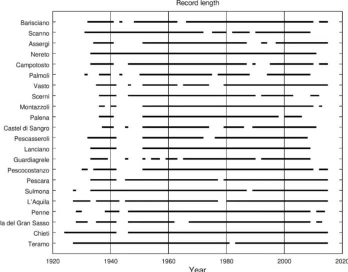
Following these restrictions, we compiled the percent-age of available data, listed in Table 1 for each station. Fig. 2 shows the availability of the raw data considering the restrictions described above: it is evident that for the period of the Second World War there is a lack of data availability in many stations, and that after about 2010 many stations were closed.
2.2.2. Fast QC of HOMER
HOMER, performing some Climatol tools, allows analysis of the main properties of the data series in
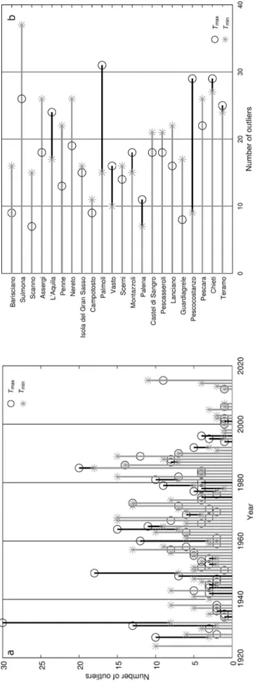
the network: the number of data points available in the network for each year, the boxplot of the temper-ature values for each month and station, a histogram with the occurrence of temperature frequency inter-vals across the whole network, a correlogram of the first difference series as function of the distance between stations and, finally, an analysis of dissimi-larity. These analyses allow further quality checks of the data relative to that described in Section 4.1. We did not identify any data quality problems at this step. The HOMER software also includes the PRODIGE analysis of outliers. We visually identified the outliers for each station, inspecting the plots generated by HOMER in which the departure from each local anomaly is compared with the average anomaly com-puted over all stations in the neighbourhood; outliers are defined when the anomaly differs from the others for a specific month and station. In our analysis, we identified 395 outliers for maximum temperatures and 416 outliers for minimum temperatures, consid-ering the whole data set of 22 stations (Fig. 3). The percentages of outliers found for each station with respect to the total available data set are shown in Table 2, which summarizes the correlation analysis between the reference series and those in the neigh-bourhood (automatically identified by HOMER) for
all stations, both before and after outlier removal. Specifically, Table 2 shows the R-values for the total data set after the first round of homogenization (i.e. for 7 homoge-nized and 15 non-homogehomoge-nized station series, see Section 2): it is evident that R-values increase after removal of the outliers.
2.2.3. Break detection
After the outliers were removed, we ran pairwise detection followed by joint detection on the QC data to identify the more evident breaks, taking into account the available metadata. We defined an inhomogeneity if at least 3 stations in the neighbourhood identified it as such, taking into account both the annual and the seasonal breaks. After the correction, we ran the ACMANT detection to confirm the inhomoge neities found with a different technique. We did not find any station series in the raw data set to be homogeneous, i.e. without inhomogeneities. In our procedure, breaks were first identified by pairwise detection; both joint detection and ACMANT detec-tion were then used to confirm these breaks. In fact, joint detection results must be treated with caution due to the problems reported by Gubler et al. (2017) and Domonkos (2017).
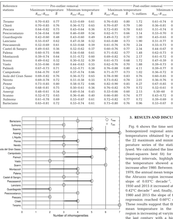
Considering that the primary objective of AC -MANT detection is to find inhomogeneities with seasonally varied biases, we used it to better iden-tify those breaks with seasonal dependence. In this case as well, we validated the seasonal breaks only if they were confirmed by pairwise detection (breaks present in at least 3 stations of the neighbourhood). We found a total of 89 and 80 inhomogeneities in the maximum and minimum temperature series, respectively (Fig. 4). All inhomogeneities found for each station are reported in Tables S1 & S2 in the Supplement at www.int-res.com/ articles/ suppl/ c077 p193_ supp. pdf, which also states if they were con-firmed by the metadata and by ACMANT detection. The majority of the 7 stations homogenized during the first step did not show any other inhomo-geneities when they were included in the second step of the homogenization, with the exception of
Stations NHS Latitude Longitude Altitude % of T
code (°N) (°W) (m a.s.l.) data
available Teramo 100 42° 39’ 17’’ 13° 43’ 2’’ 218 96.4 Chieti 1060 42° 22’ 37’’ 14° 10’ 59’’ 278 96.7 Pescara 1160 42° 26’ 58’’ 14° 14’ 32’’ 2 86.9 Pescocostanzo 1180 41° 53’ 17.5’’’ 14° 3’ 32.5’’ 1461 89.4 Guardiagrele 1240 42° 11’ 13.6’’ 14° 12’ 52.3’’ 551 77.7 Lanciano 1330 42° 13’ 32.9’’ 14° 23’ 4.1’’ 298 81.4 Pescasseroli 1350 41° 48’ 34.3’’ 13° 47’ 32.3’’ 1164 77.9 Castel di Sangro 1420 41° 46’ 51.9’’ 14° 6’ 29’’ 800 74.4 Palena 1570 41° 59’ 2.2’’ 14° 8’ 15’’ 781 72.1 Montazzoli 1680 41° 56’ 32.2’’ 14° 25’ 40.6’’ 871 80.2 Scerni 1700 42° 7’ 6.9’’ 14° 37’ 48.3’’ 125 79.1 Vasto 1740 42° 5’ 59.5’’ 14° 41’ 54.2’’ 196 82.6 Palmoli 1870 41° 56’ 30.5’’ 14° 34’ 59.8’’ 624 73.2 Campotosto 190 42° 32’ 10.1’’ 13° 24’ 23’’ 1344 85.6
Isola del Gran Sasso 260 42° 29’ 4’’ 13° 39’ 53’’ 545 83.5
Nereto 30 42° 49’ 18.6’’ 13° 48’ 46.1’’ 165 91.7 Penne 380 42° 27’ 52’’ 13° 55’ 3’’ 431 85.8 L’Aquila 550 42° 20’ 2’’ 13° 25’ 43’’ 595 92.4 Assergi 590 42° 25’ 10.7’’ 13° 31’ 5.3’’ 992 81.3 Scanno 700 41° 54’ 25’’ 13° 52’ 39’’ 1045 88.4 Sulmona 810 42° 4’ 7’’ 13° 54’ 51’’ 372 92.4 Barisciano 920 42° 19’ 25.3’’ 13° 34’ 26’’ 978 90.5 Table 1. Name, National Hydrographic Service (NHS) code, latitude, longitude, altitude and percentage of available temperature (T ) data of each station. The
Teramo station (maximum temperatures); this is highlighted in grey in Table S1. We chose to select the break points that were identified by pairwise de tection in HOMER and, when possible, confirmed them using the metadata. We did not confirm breaks suggested only by the metadata and not also supported by the statistical analysis in HOMER. We considered a break to be confirmed by metadata when the maximum difference between the breaks and the metadata was less than 2 yr. We fixed the same interval for the ACMANT detection. Tables S1 & S2 indicate the following nature of the inter -ventions, as reconstructed by the metadata: (1) a change in the altitude above sea level (a.s.l.) of the stations or in the instrument height above the ground; (2) a change in the type of instruments in use; (3) relocation; (4) a new operator for the station and (5) annotations about instrument maintenance. Unfortunately, the longest data set of available metadata (i.e. the annals) reports only changes in
altitude and instrumentation type, without reporting instrument maintenance such as calibration, inter-ventions in the stations, operators, etc. The main causes of the inhomogeneities documented by the metadata were changes in measurement techniques or station/instrument relocations. Overall, we found that (1) 47.2 and 41.3% of the inhomogeneities were confirmed by the metadata for the maximum and minimum temperatures, respectively and (2) 80.9 and 77.5% of the inhomogeneities were confirmed by the ACMANT detection analysis for the maxi-mum and minimaxi-mum temperatures, respectively. The percentage of breaks confirmed by the meta-data is in line with those found in other homoge-nization analyses: Mamara et al. (2014) found that 32% of the total inhomogeneities were confirmed by metadata information and that the majority of the metadata corresponded to breaks; Osadchyi et al. (2018) confirmed 31% of breaks by using historical information.
After the breaks were identified, we ran the ‘assess month’ function of HOMER in order to assess the positions of the identified breaks at a monthly resolution, although it must be noted that true break positions might differ from the detected break positions even when the best detection methods are used, and the detection accuracy has a statistical connection with the break magnitude (Lindau & Venema 2016). Finally, we checked the inhomo-geneities with ACMANT detection again; the percentage of confirmed ACMANT break de -tections is relative to this final check. The break highlighted by an asterisk in Table S1 was not considered as confirmed by the meta-data, because the metadata were not clearly definable.
2.2.4. Iteration and correction
The correction procedure in HOMER is an it-erative process, starting with pairwise and joint detections applied to the QC data, and then correcting them for the first time. Subsequently, we ran the same procedure again (when neces-sary), as suggested by Mestre et al. (2013). The corrections were performed with the ANOVA correction model. After a correction step, the ACMANT detection was applied to the pre-homogenized series in order to confirm the breaks highlighted by pairwise detection. The HOMER procedure cyclically proceeds be-tween correction, pairwise and joint detection on corrected series, and ACMANT detection until no more breaks are detected. In our analy-sis, we usually ran this recursive cycle between 2 and 5 times before considering the homoge-nization procedure complete.
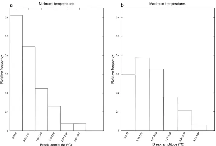
We found that all analysed series had at least one break. The annual amplitude of the breaks, expressed in absolute values, that were evaluated for the annual series are shown in Fig. 5 in terms of relative frequency distributions. The annual amplitude of the breaks in maximum temperatures ranged between 0 and 4.44°C; about 75% of the breaks had an amplitude at annual scale lower than 2.27°C (Fig. 5). For minimum tempera-tures, the break annual amplitude ranged between 0.01 and 3.75°C and about 70% of the breaks in the annual series had an annual amplitude lower than 1.35°C (Fig. 5).
Fig. 3. (a) Number of maximum (
Tmax
) and minimum (
Tmin
) temperatur
e outliers as function of year for the total data set; (b) number of
Tmax
and
Tmin
outliers identified
3. RESULTS AND DISCUSSION Fig. 6 shows the time series of the homogenized regional annual mean temperatures obtained by averaging the 22 maximum and minimum tem-perature series of the stations ana-lysed. We calculated the linear trends (least-squares best fit) for different temporal intervals, highlighting that the temperature showed an abrupt increase after 1980. Between 1924 and 1979, the annual mean temperature in the Abruzzo region increased with a slope of 0.03°C decade−1, between
1950 and 2015 it increased at a rate of 0.42°C decade−1and, finally, between
1980 and 2015 the slope of the linear regression reached 0.60°C decade−1.
These results suggest that the annual mean temperature in the Abruzzo region is increasing at varying rates in the last century with a higher rate after 1980. This is in line with what has also been found for the global Fig. 4. Inhomogeneities found for each station for both the maximum (Tmax) and
minimum (Tmin) temperatures
Reference Pre-outlier removal Post-outlier removal
stations Maximum temperature Minimum temperature Maximum temperature Minimum temperature
Rmin−Rmax R
–
Rmin−Rmax R– Rmin−Rmax R– % outliers Rmin−R max R
– % outliers Teramo 0.70−0.83 0.77 0.53−0.69 0.61 0.76−0.85 0.80 1.72 0.61−0.74 0.66 0.82 Chieti 0.70−0.85 0.76 0.56−0.72 0.65 0.70−0.87 0.79 1.00 0.56−0.81 0.67 1.09 Pescara 0.64−0.82 0.75 0.45−0.64 0.56 0.72−0.85 0.78 0.63 0.51−0.74 0.62 1.27 Pescocostanzo 0.54−0.64 0.60 0.46−0.69 0.54 0.62−0.71 0.66 3.14 0.53−0.70 0.61 0.98 Guardiagrele 0.42−0.60 0.48 0.43−0.60 0.49 0.49−0.72 0.57 1.00 0.45−0.65 0.55 2.12 Lanciano 0.55−0.67 0.62 0.47−0.58 0.52 0.65−0.88 0.73 1.90 0.51−0.77 0.62 2.62 Pescasseroli 0.52−0.69 0.61 0.53−0.68 0.59 0.61−0.76 0.70 2.24 0.55−0.73 0.65 2.61 Castel di Sangro 0.49−0.65 0.56 0.52−0.62 0.57 0.60−0.76 0.77 2.34 0.44−0.67 0.53 2.73 Palena 0.60−0.75 0.66 0.54−0.68 0.61 0.71−0.82 0.77 1.48 0.62−0.73 0.68 0.94 Montazzoli 0.59−0.74 0.64 0.51−0.72 0.60 0.69−0.82 0.74 2.17 0.61−0.72 0.69 1.81 Scerni 0.49−0.62 0.52 0.30−0.52 0.39 0.61−0.75 0.68 1.72 0.47−0.59 0.53 1.96 Vasto 0.55−0.66 0.60 0.44−0.63 0.55 0.62−0.76 0.70 1.88 0.59−0.73 0.65 1.17 Palmoli 0.67−0.73 0.71 0.52−0.71 0.58 0.76−0.88 0.80 4.11 0.59−0.77 0.69 1.99 Campotosto 0.64−0.70 0.67 0.57−0.74 0.66 0.71−0.77 0.73 1.02 0.56−0.72 0.65 1.25
Isola del Gran Sasso 0.69−0.82 0.76 0.56−0.72 0.65 0.78−0.90 0.83 0.76 0.60−0.85 0.71 0.45
Nereto 0.69−0.78 0.72 0.51−0.58 0.55 0.73−0.82 0.78 2.01 0.56−0.76 0.62 2.75 Penne 0.73−0.85 0.80 0.58−0.72 0.66 0.82−0.90 0.85 0.27 0.67−0.85 0.74 1.00 L’Aquila 0.68−0.81 0.75 0.50−0.61 0.56 0.76−0.82 0.79 0.72 0.52−0.61 0.57 0.27 Assergi 0.48−0.61 0.54 0.40−0.54 0.45 0.53−0.66 0.60 2.15 0.50−60 0.55 3.10 Scanno 0.52−0.72 0.65 0.36−0.46 0.40 0.66−0.80 0.74 0.77 0.43−0.72 0.51 1.64 Sulmona 0.61−0.78 0.69 0.53−0.67 0.61 0.72−0.82 0.77 0.72 0.59−0.69 0.63 0.54 Barisciano 0.65−0.81 0.72 0.53−0.74 0.61 0.73−0.80 0.76 0.96 0.53−0.67 0.61 1.71
Table 2. Correlation coefficient analysis for the complete temperature data set. The 7 stations homogenized in the first step are written in
italics. Correlations (R-values) were evaluated between each reference station (listed in the first column) and the first 6 best correlated stations of the neighbourhood
mean temperature (Trenberth et al. 2007, Hartmann et al. 2013). We compared our results with tempera-ture trends that have been found for similar regions in the Mediterranean area. Antolini et al. (2016) ana-lysed the mean temperature trend over the Emilia-Romagna region (300 km north of the sites analysed in this study), reporting increases at some stations of up to 0.5°C decade−1(1961−2010). Furthermore, Mar-letto et al. (2009) produced a hydro-climatic atlas for the Emilia-Romagna region, evaluating increasing trends during the period 1961−2008 of 0.25 and 0.46°C decade−1 for minimum and maximum mean
temperatures, respectively. The Annual Bulletin on the Climate in WMO Region VI (DWD 2011) showed the trend analysis map for annual temperatures (1951−2011) and re vealed that, in the region of inter-est (central-southern Italy), the trends were greater than 0.3°C decade−1. Finally, Liuzzo et al. (2017)
investigated the long-term temperature changes in Sicily during the 1924− 2013 period and indicated that at some sites, the maximum temperature had a positive trend of 0.5°C decade−1. Fig. 7 depicts the
Fig. 5. Annual amplitude of the breaks, in absolute values, for the (a) minimum and (b) maximum temperatures, expressed as relative frequency distributions
Fig. 6. Annual mean temperatures for the Abruzzo region (obtained by averaging the maximum and minimum tem-perature series of all stations). A linear regression model (least-squares best fit) was applied in different temporal intervals in order to find the slopes as function of period in
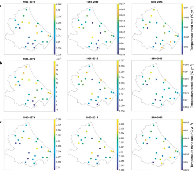
spatial distribution of the temperature trends in the Abruzzo region, showing the slopes of linear regres-sion for the annual mean temperatures (Fig. 7a), the maximum temperatures (Fig. 7b) and the minimum temperatures (Fig. 7c), evaluated over 3 different time periods: 1930−1979, 1950−2015 and 1980−2015. The local variability of the rate of temperature change is quite pronounced and differs among the different time intervals as well as for the maximum, minimum and annual mean temperatures. One exam-ple of this difference is that in the first period consid-ered (1930−1979), the rate of temperature change
was slightly higher in the coast-hill parts of the region compared to mountain areas, whereas in the periods 1950−2015 and 1980−2015, the variations were more scattered with less evidence of definite areas having higher changes than others. These results confirm the importance of using homogenized data series of maximum and minimum temperatures to better describe the local impact of climate change and regional temperature trends. It is evident that some sites (such as Pescara and Teramo in Fig. 7, with increases of 0.9°C decade−1) in the 1980−2015
period present greater increasing temperature trends
Fig. 7. Spatial temperature trend rates of the Abruzzo region: (a) annual mean temperature, (b) maximum temperature and (c) minimum temperature. The slopes of linear regression models, applied to the homogenized data set of 22 series, have been
than that at the regional level (0.78°C decade−1).
Moreover, the difference between local and regional trends is more variable in the 1980− 2015 period com-pared to the 1950−2015 period. It is also evident that in some sites (such as Castel di Sangro in Fig. 7, with an increase of about 0.7°C decade−1) the major
impact is on the minimum temperatures, since the annual mean temperature trends (1980−2015) were greater than the regional annual mean trend (0.6°C decade−1).
4. CONCLUSIONS
We homogenized the series of maximum and mini-mum temperatures recorded at 22 different sites (mountains, valleys, hills and sea coast) in the Ab -ruzzo region (central Italy). With the application of the software HOMER, we identified 395 and 416 out-liers in the maximum and minimum temperatures, respectively. The pairwise, joint and ACMANT de -tection analyses allowed us to detect a total of 89 and 80 breaks in the maximum and minimum tempera-ture series, respectively. About 47.2 and 41.3% of the inhomogeneities were confirmed by the metadata for the maximum and minimum temperatures, respec-tively. About 80.9 and 77.5% of the inhomogeneities were confirmed by the ACMANT detection analysis for the maximum and minimum temperatures, re -spectively. The lack of metadata did not allow us to verify more breaks, but the correspondence between the pairwise and ACMANT detection results con-firmed that the detected breaks were relevant. The homogenized data set covers a gap of temperature data over the period 1930−2015 in central Italy, extending from the coast of the Adriatic Sea to high mountain areas; hence, this information will enrich the Greater Mediterranean area temperature series with a long-term and high-quality surface data set that can be used for climate-related assessments and for climate products and services. Spatial hetero-geneities of minimum, maximum and annual mean temperature changes across the different temporal intervals analysed are highlighted, showing the pres-ence of different trends between the coastal and mountain regions during the period 1930−1979.
Acknowledgements. We thank Mario Cerasoli and Antonio
Iovino of the Centro Funzionale of Abruzzo Region, for access to their temperatures database and for supporting us in the metadata reconstruction. Moreover, we thank Dr. Mestre and Dr. Dubuisson (Meteo France) for their help in the use of the HOMER software. This work was partially sup-ported by Fondi di Ricerca Dipartimentali (DiSPuTer − 2017).
LITERATURE CITED
Aguilar E, Auer I, Brunet M, Peterson TC, Wieringa J (2003) Guidelines on climate metadata and homogenization. World Meteorological Organization Technical Document No. 1186. WMO, Geneva
Alexandersson H (1986) A homogeneity test applied to pre-cipitation data. Int J Climatol 6: 661−675
Alexandersson H, Moberg A (1997) Homogenization of Swedish temperature data. I. Homogeneity test for linear trends. Int J Climatol 17: 25−34
Allen R, Pereira L, Raes D, Smith M (1998) Statistical analy-sis of weather data sets, crop evapotranspiration — guidelines for computing crop water requirements. Irri-gation and Drainage Paper No. 56. FAO, Rome
Antolini G, Auteri L, Pavan V, Tomei F, Tomozeiu R, Mar-letto V (2016) A daily high-resolution gridded climatic data set for Emilia-Romagna, Italy, during 1961−2010. Int J Climatol 36: 1970−1986
Auer I, Böhm R, Schöner W, Hagen M (1999) ALOCLIM− Austrian−central European long-term climate — creation of a multiple homogenized long-term climate data-set. In: Proc 2ndseminar for homogenisation of surface
clima-tological data, 9−13 November 1998, Budapest. WMO, Budapest, p 47−71
Beaulieu C, Ouarda TBMJ, Seidou O (2010) A Bayesian normal homogeneity test for the detection of artificial discon -tinuities in climatic series. Int J Climatol 30: 2342−2357 Brunet M, Jones PD, Jourdain S, Efthymiadis D, Kerrouche
M, Boroneant C (2014) Data sources for rescuing the rich heritage of Mediterranean historical surface climate data. Geosci Data J 1: 61−73
Brunetti M, Maugeri M, Monti F, Nanni T (2006) Tempera-ture and precipitation variability in Italy in the last two centuries from homogenised instrumental time series. Int J Climatol 26: 345−381
Caussinus H, Mestre O (1996) New mathematical tools and methodologies for relative homogeneity testing. In: Proc 1stseminar for homogenization of surface climatological
data, 6−12 October 1996, Budapest. Hungarian Meteoro-logical Service, Budapest, p 63−82
Caussinus H, Mestre O (2004) Detection and correction of artificial shifts in climate series. Appl Stat 53: 405−425 Costa AC, Negreiros J, Soares A (2008) Identification of
inhomogeneities in precipitation time series using stochastic simulation. In: Soares A, Pereira MJ, Dimitrako -poulos R (eds) geoENV VI: geostatistics for environmen-tal applications. Springer, Heidelberg, p 275−282 Craddock JM (1979) Methods of comparing annual rainfall
records for climatic purposes. Weather 34: 332−346 Domonkos P (2011) Adapted Caussinus-Mestre algorithm
for networks of temperature series (ACMANT). Int J Geosci 2: 293−309
Domonkos P (2014) The ACMANT2 software package. In: Lakatos M, Szentimrey T, Marton A (eds) Eighth seminar for homogenization and quality control in climatological databases and third conference on spatial interpolation techniques in climatology and meteorology, 12−16 May 2014, Budapest. WCDMP No. 84. WMO, Geneva, p 46−72
Domonkos P (2017) Time series homogenisation with opti-mal segmentation and ANOVA correction: past, present and future. In: Szentimrey T, Lakatos M, Hoffmann L (eds) Ninth seminar for homogenization and quality con-trol in climatological databases and fourth conference on
spatial interpolation techniques in climatology and mete-orology, 3−7 April 2017, Budapest. WCDMP No. 85. WMO, Geneva, p 29−45
Domonkos P, Coll J (2017) Homogenisation of temperature and precipitation time series with ACMANT3: method description and efficiency tests. Int J Climatol 37: 1910−1921
DWD (Deutscher Wetterdienst) (2011) Annual bulletin on the climate in WMO Region VI — Europe and Middle East. DWD, Offenbach am Main
Gubler S, Hunziker S, Begert M, Croci Maspoli M and others (2017) The influence of station density on climate data homogenization. Int J Climatol 37: 4670−4683 Guijarro J (2006) Homogenization of a dense
thermo-pluvio-metric monthly database in the Balearic Islands using the free contributed R package ‘climatol’. In: Lakatos M, Szentimrey T, Bihari Z, Szalai S (eds) Proc 5thseminar for
homogenization and quality control in climatological databases, 29 May−2 June 2006, Budapest. WCDMP No. 71. WMO, Geneva, p 25−36
Guijarro JA (2011) User’s guide to climatol. An R contributed package for homogenization of climatological series. www.climatol.eu/climatol-guide.pdf
Guijarro JA (2018) Homogenization of climatic series with Climatol. www.climatol.eu/homog_climatol-en.pdf Hartmann DL, Klein Tank AMG, Rusticucci M, Alexander
LV and others (2013) Observations: atmosphere and sur-face. In: Stocker TF, Qin D, Plattner GK, Tignor M and others (eds) Climate change 2013: the physical science basis. Contribution of Working Group I to the Fifth Assessment Report of the Intergovernmental Panel on Climate Change. Cambridge University Press, Cam-bridge, p 159−254
ISPRA (2017) Stato dell’Ambiente — Gli indicatori del clima in Italia nel 2015, ISPRA, Stato dell’Ambiente 72/2017 (in Italian)
Lindau R, Venema V (2016) The uncertainty of break posi-tions detected by homogenization algorithms in climate records. Int J Climatol 36: 576−589
Liuzzo L, Bono E, Sammartano V, Freni G (2017) Long-term temperature changes in Sicily, southern Italy. Atmos Res 198: 44−55
Mamara A, Argiriou AA, Anadranistakis M (2014) Detection and correction of inhomogeneities in Greek climate tem-perature series. Int J Climatol 34: 3024−3043
Marletto V, Antolini G, Tomei F, Pavan V, Tomozeiu R (2009) Atlante idroclimatico dell’Emilia-Romagna 1961–2008. ARPA Emilia-Romagna, Bologna. www.arpa.emr.it/sim/? clima (accessed 8 May 2015)
Menne MJ, Williams CN Jr (2009) Homogenization of tem-perature series via pairwise comparisons. J Clim 22: 1700−1717
Mestre O, Domonkos P, Picard F, Auer I and others (2013) HOMER: a homogenization software — methods and ap -plications. Q J Hung Meteorol Ser 117: 47−67
Osadchyi V, Skrynyk O, Radchenko R, Skrynyk O (2018) Homogenization of Ukrainian air temperature data. Int J Climatol 38: 497−505
Pettitt AN (1979) A non-parametric approach to the change-point problem. Appl Stat 28: 126−135
Picard F, Lebarbier E, Hoebeke M, Rigaill G, Thiam B, Robin S (2011) Joint segmentation, calling, and normalization of multiple CGH profiles. Biostatistics 12: 413−428 Ribeiro S, Caineta J, Costa AC (2016) Review and discussion
of homogenisation methods for climate data. Phys Chem Earth 94: 167−179
Ribeiro S, Caineta J, Costa AC, Henriques R (2017) gsimcli: a geostatistical procedure for the homogenisation of climatic time series. Int J Climatol 37: 3452−3467 Scorzini AR, Di Bacco M, Leopardi M (2018) Recent trends
in daily temperature extremes over the central Adriatic region of Italy in a Mediterranean climatic context. Int J Climatol 38(Suppl 1): e741−e757
Szentimrey T (1999) Multiple Analysis of Series for Homog-enization (MASH). In: Proc 2ndseminar for
homogeniza-tion of surface climatological data, 9−13 November 1998, Budapest. WCDMP No. 41. WMO, Geneva, p 27−46 Toreti A, Desiato F (2008) Temperature trend over Italy from
1961 to 2004. Theor Appl Climatol 91: 51−58
Trenberth KE, Jones PD, Ambenje P, Bojariu R and others (2007) Observations: surface and atmospheric climate change. In: Solomon S, Qin D, Manning M, Chen Z and others (eds) Climate change 2007: the physical science basis. Contribution of Working Group I to the Fourth Assessment Report of the Intergovernmental Panel on Climate Change. Cambridge University Press, Cam-bridge, p 235−336
Venema VKC, Mestre O, Aguilar E, Auer I and others (2012) Benchmarking homogenization algorithms for monthly data. Clim Past 8: 89−115
Wang XL (2008) Accounting for autocorrelation in detecting mean shifts in climate data series using the penalized maximal t or F test. J Appl Meteorol Climatol 47: 2423−2444
WMO (2011) Guide to climatological practices, Vol 100. World Meteorological Organization, Geneva
WMO (2016) WMO Climatological Standard Normals, Chapter 4, Item 4.8 (updated 19.01.2016). World Mete -orological Organization, Geneva
Editorial responsibility: Eduardo Zorita, Geesthacht, Germany
Submitted: July 24, 2018; Accepted: December 20, 2018 Proofs received from author(s): February 22, 2019