Design and Performance Evaluation of Residual Generators for the FDI of an Aircraft

DOI: 10.1007/s10453-004-5872-7

Design and Performance Evaluation of Residual

Generators for the FDI of an Aircraft

Marcello Bonf`e

_{Paolo Castaldi}

_{Walter Geri}

_{Silvio Simani}

Abstract: In this work, several procedures for the fault detection and isolation (FDI) on general aviation aircraft sensors are presented. In order to provide a comprehensive wide–spectrum treatment, both linear and nonlinear, model–based and data–driven methodologies are considered. The main contributions of the paper are related to the development of both FDI polynomial method (PM) and FDI scheme based on the nonLinear geometric approach (NLGA). As to the PM, the obtained results highlight a good trade–off between solution complexity and resulting performances. Moreover, the proposed PM is especially useful when robust solutions are required for minimising the effects of modelling errors and noise, while maximising fault sensitivity. As to the NLGA, the proposed work is the first development and robust application of the NLGA to an aircraft model in flight conditions characterised by tight–coupled longitudinal and lateral dynamics. In order to verify the robustness of the residual generators related to the previous FDI techniques, the simulation results adopt a typical aircraft reference trajectory embedding several steady–state flight conditions, such as straight flight phases and coordinated turns. Moreover, the simulations are performed in the presence of both measurement and modelling errors. Finally, extensive simulations are used for assessing the overall capabilities of the developed FDI schemes and a comparison with neural networks (NN) and unknown input Kalman filter (UIKF) diagnosis methods is performed.

Keywords: Fault diagnosis, dynamic filters, polynomial method(PM), input–output sensors, aircraft simulated model.

1

Introduction

The control devices currently in use to improve the over-all performance of aircraft systems involve both sophisti-cated digital system design techniques and complex hard-ware (sensors, actuators, processing units). The complexity means that the probability of fault occurrence can be signif-icant and an automatic supervisory control system should be used to detect and isolate anomalous working conditions as early as possible. These motivations pushed a great at-tention on fault detection and isolation (FDI) in dynamic processes and a wide variety of so–called model–based ap-proaches have been proposed[1−4]_{. Model–based methods}

all use mathematical models of the plant being monitored. However, the conceptual realization of these models can vary according to the following approaches: the parity space[5]_{, state estimation}[6]_{, unknown input observer (UIO)}

and Kalman filters (KF)[1] _{and parameter identification}[6]_.

Intelligent techniques[7]_{can be also exploited.}

For the case of model–based approaches, to guarantee that faults can be detected and isolated (and distinguish-able), mathematical models of the process under investi-gation are required, either in state space or input–output forms. Residuals should then be processed to detect an actual fault condition to reject any false alarms caused by noise or spurious signals. However, in practical appli-cations, especially when considering aircraft systems, the straightforward application of such FDI techniques can be difficult. In fact, the plant model is usually designed to carefully capture all kinds of details relevant to the anal-ysis and deployment of the real system. Thus, this model is often nonlinear and complex to describe accurately the

Manuscript received February 21, 2006; revised December 18, 2006. *Corresponding author. E-mail address: silvio.simani@unife.it

behaviour of the real target system. Moreover, presence of disturbances, modelling and measurement errors cannot be neglected. This intrinsic complexity, however, makes almost unfeasible the straightforward application of many cited FDI methods, and a viable procedure for practical application of FDI techniques is really necessary. Although many linear and nonlinear approaches have been developed, robust FDI for the case of aircraft systems and aerospace applications is still an open problem for further research.

This work deals with the residual generator design for the FDI of onboard sensors of a general aviation aircraft subject to turbulence, wind gust disturbances and measure-ment noises. As to PM, the proposed method is based on an input–output polynomial description of the system un-der diagnosis. In this way, the design of disturbance de-coupled residual generators can be reduced to the deter-mination of the null–space of a specific polynomial matrix associated to the process model. In particular, the use of input–output forms allows to easily obtain the analytical description for the disturbance decoupled residual genera-tors. These dynamic filters, organised into bank structure, are able to achieve fault isolation properties. An appropri-ate choice of their parameters allows to maximise robustness with respect to both measurement noise and modelling er-rors, while optimising fault sensitivity characteristics. As to NLGA, the proposed FDI scheme is based on the recently methodology developed in [8,9]. Such a method has been applied for the first time in [10] to a VTOL aircraft with reference to a reduced–order model, by constraining also the motion on the vertical–lateral plane. Moreover, in that applicative seminal work no wind effects or engine model has been considered. In [11], instead, the design of residual generators based on the NLGA with respect to just the lon-gitudinal dynamics (3DoF aircraft model) of a general

avi-ation aircraft can be found. Even though both the present work and [10,11] have a common framework, the present paper provides a generalisation to an aircraft model based on a 6 degrees of freedom (6 DoF) rigid body formulation and the aim is to carry out the FDI even if the flight con-ditions are not compliant with the hypothesis of decoupled longitudinal and lateral–directional dynamics. Moreover, the NLGA residual generators have been designed in order to be analytically decoupled from the vertical and lateral components of the wind (gusts and turbulence).

The residual generators of the proposed approaches have been tested on a PIPER PA–30 aircraft flight simula-tor, implemented in Matlabr_{and Simulink}r_{environments.}

The simulation model, detailed in [11], is made up of a 6DoF rigid body structure as well as the models of wind gusts, Dryden atmospheric turbulence, measurement sen-sors, servo actuators and a classical autopilot.

The robustness of the proposed FDI schemes with respect to model errors and disturbances has been evaluated by adopting a typical aircraft reference trajectory embedding several steady–state flight conditions, such as straight flight phases and coordinated turns. Finally, a comparison with neural networks (NN) and unknown input Kalman filter (UIKF) diagnosis methods is provided.

The paper is organised as follows. Section 2 presents the PM FDI scheme. In Section 3 a brief description of the NLGA FDI scheme is reported. In Section 4 the effective-ness of the proposed filter generators applied to a PIPER PA–30 flight simulator and some numerical results are re-ported. Finally, Section 5 summarises the contributions and achievements of the paper and provides some suggestions for possible further research topics.

2

PM residual generators

Let’s consider a linear, time–invariant, continuous–time system described by the following input–output model:

P (s) y(t) = Q(s) u(t) (1) where s is the derivative operator and P (s) and Q(s) are polynomial matrices with dimensions (m × m) and (m × `) respectively, with P (s) nonsingular. The terms u(t) and

y(t) are the `–dimensional and m–dimensional input and

output vectors of the considered multivariable system. The residual generators can be obtained by partitioning the matrix Q(s) according to the following structure:

P (s) y(t) = h Qc(s) Qd(s) Qf(s) i 2 6 4 c(t) d(t) f (t) 3 7 5 (2)

where c(t) is the `c–dimensional control input vector, d(t) is the `d–dimensional disturbance unknown vector, f (t) is the

`f–dimensional monitored fault vector and `c+ `d+ `f = `. The general linear residual generator for the FDI of (2) is a filter of type:

R(s) r(t) = Sy(s) y(t) + Sc(s) c(t). (3) If r(t) is a scalar signal, R(s) has to be a polynomial with degree greater than or equal to the row–degree of Sc(s) and

Sy(s).

The decoupling of the disturbance d(t) can be obtained as follows. If the model (2) is rewritten in the form:

P (s) y(t) − Qc(s) c(t) − Qf(s) f (t) = Qd(s) d(t) (4) premultiplying all the terms in (4) by a row polynomial vector L(s) ∈ N`(Qd(s)), which belongs to the left null– space of Qd(s), the relation (5) is obtained:

L(s) P (s) y(t) − L(s) Qc(s) c(t) − L(s)Qf(s) f (t) = 0 . (5) When f (t) = 0, the residual generator is obtained (3) by setting Sy(s) = L(s) P (s) Sc(s) = −L(s) Qc(s) R(s) = (1 + τ1s)(1 + τ2s)..(1 + τnfs) = = a1snf + a2snf−1+ .. + 1 (6)

where nf is the maximal row–degree of the pair ˘

L(s) P (s), L(s) Qc(s) ¯

. The polynomial R(s) can be ar-bitrarily selected, even if the choice of R(s) has a direct influence on the properties of the filter[11]_.

When a fault is acting on the system, the residual gen-erator is governed by the relation:

R(s) r(t) = L(s) Qf(s) f (t) (7) and r(t) assumes values that are different from zero if L(s) does not belong to the N`(Qf(s)).

The diagnostic capabilities of the residual generator (3) and (7) strongly depend also on the matrix L(s). For ex-ample, when m − `d > 1, the design freedom can be used to optimise the sensitivity properties of r(t) to the fault

f (t). Regarding the location of the roots of the polynomial R(s) in the left–half s–plane, they influence the transient

characteristics (maximum overshoot, delay time, rise time, settling time, etc.) of the filter (7) with respect to unit–step response.

Regarding the fault typology, it is worth noting that the model (2) considers also the cases of additive faults on the input and output sensors, fc(t) and fo(t), respectively. In this situation only the measurements

c∗_{(t) = c(t) + f}

c(t) (8)

y∗(t) = y(t) + fo(t) (9) are available for the residual generators so that (3) becomes

R(s) r(t) = L(s) P (s) y∗(t) − L(s) Qc(s) c∗(t) = 0 (10) in the absence of faults and

R(s) r(t) = L(s) Qc(s) fc(t) − L(s) P (s) fo(t) (11) when faults on input–output sensors are considered.

Once the residual generation task has been accomplished, the problem of isolation of faults affecting the input and out-put sensors has to be solved. The design is performed by us-ing banks of residual generation filters and the disturbance decoupling method previously suggested. In the following it is assumed that m > `d+ 1. In particular, regarding the

input sensor fault isolation, under the hypothesis that all

filters is used. The number of these generators is equal to the number `c of system control inputs, and the i–th de-vice (i = 1, . . . , `c) is driven by all but the i–th input and all the outputs of the system. In this case, a fault on the

i–th input sensor affects all but the i–th residual generator.

Similar considerations can be applied to design a bank of residual generators to univocally isolate a fault concerning one of the output sensors. More design details can be found in [11].

Once the residuals have been generated, the residual evaluation logic is used to detect and isolate any fault oc-currence. The residual processing methods can be based on simple residual geometrical analysis or comparison with fixed thresholds[1]_{. More complex residual evaluation tests}

can also be exploited, e.g., based on statistical properties of the residuals and hypothesis testing, as discussed in [6]. In general, in the absence of faults, the residual signals are approximately zero. In practical situations, the residual is never zero, even no faults occur. A threshold must then be used and normally is set suitably larger than the largest magnitude of the residual for the fault–free case. The small-est detectable fault is a fault which drives the residual func-tion to just exceed the threshold. Any fault producing a residual response smaller than this magnitude is not de-tectable. More in detail, the most widely used way to fault detection is achieved by directly comparing residual signal

r(t) or a residual function J (r(t)) with a fixed threshold ε

or a threshold function ε(t) as follows: 8 > < > : J (r(t)) ≤ ε(t) for f (t) = 0 J (r(t)) > ε(t) for f (t) 6= 0 (12)

where f (t) is the general fault vector. If the residual exceeds the threshold, a fault may be occurred. This test works especially well with fixed threshold ε if the process operates approximately in steady state and it reacts after relatively large feature, i.e., after either a large sudden or a long– lasting gradually increasing fault.

In practice, if the residual signal is represented by the stochastic variable r(t), mean value and variance are com-puted as follows: 8 > > > > < > > > > : ¯ r = E{r(t)} = 1 N N P t=1 r(t) σ2 r= E{[r(t) − ¯r]2} = _N1 N P t=1 [r(t) − ¯r]2 (13) where ¯r and σ2

rare the normal values for the mean and vari-ance of the fault–free residual, respectively. N is the num-ber of samples of the vector r(t). Therefore, the threshold test for FDI of (12) is rewritten as

8 > < > : ¯ r − δ σr≤ r(t) ≤ ¯r + δ σr for f (t) = 0 r(t) < ¯r − δ σr or r(t) > ¯r + δ σr for f (t) 6= 0 (14)

i.e., the comparison of r(t) with respect to its statistical normal values. In order to separate normal from faulty be-haviour, the tolerance parameter δ (normally δ ≥ 2) is se-lected and properly tuned. Hence, by a proper choice of the

parameter δ, a good trade–off can be achieved between the maximisation of fault detection probability and the minimi-sation of false alarm rate. Hence, the freedom design in the selection of the polynomial matrices L(s) and R(s) is used for optimising the sensitivity properties of r(t) to the fault

f (t), i.e., by optimising both the fault sensitivity and the

disturbance rejection. Another design choice regards the value of δ for the residual evaluation stage. This param-eter influences the FDI capabilities via (14). In practical applications, these thresholds should lead to tolerable or prescribed limits, in order to guarantee good performance of the filter in terms of FDI probabilities, fault detection time and false alarm rates.

The generation and evaluation of analytic symptoms con-clude the FDI task within the framework of model–based fault diagnosis.

3

NLGA residual generators

The proposed NLGA FDI scheme requires a model struc-ture of the input affine type[9]_{, but the adopted simulation}

model does not meet this requirement. For this reason, the following simplified aircraft model (FDI model) is used to design the residual generators:

˙ V = − ` CD0+ CDαα + CDα2α2 ´ m V 2₊

g (sin α cos θ cos φ − cos α sin θ) +

cos α m tp V (t0+ t1ne) δth+ wvsin α ˙α = −(CL0+ CLαα) m V + g

V (cos α cos θ cos φ + sin α sin θ) + qω−

sin α m tp V2(t0+ t1ne) δth+ cos α V wv ˙ β = ` CD0+ CDαα + CDα2α2 ´

sin β + CYββ cos β

m V + gcos θ sin φ V + pωsin α − rωcos α− cos α sin β m tp V2(t0+ t1ne) δth+ 1 Vw` ˙pω=(Clββ + Clppω) Ix V2₊(Iy− Iz) Ix qωrω+Cδa Ix V2_δ a ˙qω=(Cm0+ Cmαα + Cmqqω) Iy V2₊(Iz− Ix) Iy pωrω+ Cδe Iy V2_δ e+ td Iy tp V (t0+ t1ne) δth ˙rω= (Cnββ + Cnrrω) Iz V2₊(Ix− Iy) Iz pωqω+ Cδr Iz V2_δ r ˙

φ = pω+ (qωsin φ + rωcos φ) tan θ

˙θ = qωcos φ − rωsin φ ˙ ψ = (qωsin φ + rωcos φ) cos θ ˙ne= tnn3e+ tf ne (t0+ t1ne) δth (15)

where V is the true–air–speed; α and β are the angles of attack and sideslip; pω, qω, rω are the roll, pitch and yaw rates; φ, θ, ψ are the bank, elevation and heading angles; ne is the engine shaft angular rate; δe, δa, δr are the elevator, aileron and rudder deflection commands; δthis the throttle

command; m, g are the mass and the gravity acceleration;

Ix, Iy, Izare the inertia moments; C(·)are the aerodynamic

coefficients; t(·) are the engine parameters; wv, wlare the vertical and lateral wind disturbance components.

The FDI model and residual generators have been ob-tained on the basis of the following main assumptions:

1) the faults affect the most critical aircraft sensor set, in particular the input sensors associated to the elevator, aileron, rudder and throttle.

2) the expressions of aerodynamic forces and moments have been represented by means of series expansions in the neighbourhood of the steady–state flight condition, then only the main terms are considered.

3) the engine model has been simplified by linearising the power with respect to the angular rate behaviour in the neighbourhood of the trim point.

4) the second order coupling between the longitudinal and lateral–directional dynamics has been neglected.

5) the x–body axis component of the wind has been ne-glected. In fact, the aircraft behaviour is much more sensi-tive to the y–body and z–body axis wind components.

6) the rudder effect in the equation describing the β dy-namics has been neglected.

The next designs will show that the residual generators are robust with respect to the last approximation. In fact, the model of the β dynamics will never be used.

The elevator residual generator rδe(t), with Kδe> 0, is

8 > > > > > > > > > > > > > > > > > < > > > > > > > > > > > > > > > > > : ˙ξ1= V2 m ˆ −`CD0+ CDαα + CDα2α2 ´ cos α˜+ V2 m (CL0+ CLαα) sin α − g sin θ− V qωsin α −(Cm0+ Cmαα + Cmqqω) mtd V2₋ (Iz− Ix) mtd pωrω− Cδe mtd V2_δ e+ Kδe »„ V cos α − Iy mtd qω « − ξ1 – rδe= „ V cos α − Iy mtd qω « − ξ1 . (16)

The aileron residual generator rδa(t), with Kδa> 0, is

8 > > > > < > > > > : ˙ξ2 =(Clββ + Clppω) Ix V2₊(Iy− Iz) Ix qωrω+ Cδa Ix V 2 δa+ Kδa(pω− ξ2) rδa = pω− ξ2 . (17)

The rudder residual generator rδr(t), with Kδr> 0, is

8 > > > > < > > > > : ˙ξ3=(Cnββ + Cnrrω) Iz V 2 +(Ix− Iy) Iz pωqω+ Cδr Iz V2_δ r+ Kδr(rω− ξ3) rδr = rω− ξ3 . (18)

The throttle residual generator rδ_th(t), with Kδ_th > 0, is 8 > > < > > : ˙ξ4 = tnn3e+ tf ne (t0+ t1ne) δth+ Kδth(ne− ξ4) rδ_th = ne− ξ4 . (19)

The design of the residual generator gains Kδe, Kδa, Kδr

and Kδth can be carried out independently. The aim is to

optimise the trade–off between the fault sensitivity and the robustness to the modelling errors and disturbances. It is worth observing that the gain design can be achieved by experimental tests of low computational burden , because of the scalar dimension of each residual generator design problem.

4

FDI performance evaluation

To show the diagnostic characteristics brought by the application of the proposed FDI schemes to general aviation aircrafts, some numerical results obtained in the Matlab°R

and Simulink°R _{environment are reported.}

This section firstly recalls briefly the description of the monitored aircraft. Then, the final performances that are achieved with the developed FDI schemes are reported. These performances are evaluated by means of extensive simulations applied to the aircraft simulation model. This section presents also some comparisons of the developed PM and NLGA FDI strategies with NN and UIKF FDI schemes. The considered aircraft simulation model consists of a PIPER PA–30, based on the classical nonlinear 6 DoF rigid body formulation[12]_{, whose motion occurs as a consequence}

of applied forces and moments (aerodynamic, propulsive and gravitational). A set of local approximations for these forces has been computed and scheduled depending on the values assumed by true air speed (TAS), curvature radius, flight path angle, altitude and flap deflection. In this way, it is possible to obtain a mathematical model for each flight condition. This model is suitable for a state–space represen-tation, as it can be made explicit. The parameters in the an-alytic representation of the aerodynamic actions have been obtained from wind tunnel experimental data, and the aero-dynamic actions are expressed along the axes of the wind reference system. It should be observed that aerodynamic forces and moments are not implemented by the classical linearised expressions (stability derivatives) but by means of cubic splines approximating the nonlinear experimental curves. The nonlinear 6 DoF model has been completed by means of the PIPER PA–30 propulsion system consist-ing of two 4–pistons aspirated engines, with the throttle valve aperture δthas input and the overall thrust intensity as output. The overall simulation model, used to perform all the following tests, consists of the aircraft 6 DoF flight dynamics and the engine model completed with the model of sensors, servo actuators, atmosphere turbulence Dryden description, wind gust disturbances and a classical autopi-lot. Moreover, the sensor models embed all the possible sources of disturbance (calibration and alignment errors, scale factor, white and coloured noises, limited bandwidth, g–sensitivity, gyro drift, etc.).

The linear model used by the proposed PM FDI approach embeds the linearisation of both the 6 DoF model and the propulsion system as follows:

with x(t) =ˆ∆V (t) ∆α(t) ∆β(t) ∆pω(t) ∆qω(t) ∆rω(t) . . . . . . ∆φ(t) ∆θ(t) ∆ψ(t) ∆H(t) ∆ne(t) ˜T c(t) =ˆ∆δe(t) ∆δa(t) ∆δr(t) ∆δth(t) ˜T d(t) =ˆwu(t) wv(t) ww(t) ˜T (21)

where ∆ denotes the variations of the considered variables, while c(t) and d(t) are the control inputs and the distur-bances respectively. The output equation associated to the model (20) is of the type y(t) = CCC x(t), where the rows of C

C

C correspond to rows of the identity matrix, depending on

the measured variables.

It is worth noting that the aircraft reference trajectories are typically made up of a sequence of steady–state flight conditions, each one described by the associated input– state–output set point and the linearised model of type (20). As a consequence, all the FDI linear techniques are usually implemented by switching among the residual generators related to the different steady–state flight conditions. The target of this work is to reduce the switching by adopting robust PM residual generators. In particular, the robust-ness is achieved by using the same residual generators for a large set of flight conditions.

The designed PM residual generator filters are fed by the 4-component input vector c(t) and the 11-component out-put vector y(t) acquired from the simulation aircraft model previously described. In particular, a bank of 4 residual generator filters has been used to detect input sensor faults regarding the 4 input control variables. Moreover, in order to obtain the fault isolation properties, each residual gen-erator function of the considered bank is fed by all but one the 4 control input signals and by the 11 output variables. Obviously, the residual generator bank has been designed to be decoupled with the 3-component wind disturbance vector d(t) = [wu(t), wv(t), ww(t)]T.

As to the NLGA residual generator filters, the aircraft synthesis model (15), adopted for the design, is simplified with respect to the simulation model. Analogous to the PM, the approximations of the NLGA synthesis nonlinear model are related to a particular steady–state flight con-dition. For this reason, the switching for the NLGA FDI scheme is also required when a generic reference trajectory is followed. Hence, it is important to evaluate the robust-ness characteristic of a single design of NLGA residual gen-erators when a large set of flight conditions is dealt with.

The chosen single steady–state flight condition for the design of both the PM and the NLGA residual generators is a coordinated turn characterised as follows:

1) the true–air–speed is 50 m/s 2) the curvature radius is 1000 m 3) the flight–path angle is 0◦ 4) the altitude is 330 m 5) the flap deflection is 0◦_.

This represents one of most general flight condition, due to the coupling of the longitudinal and lateral dynamics. Moreover, it is used in simulation to highlight the perfor-mances of the proposed methods in the nominal flight con-dition.

As to the PM, the detection properties of the filters in

terms of fault sensitivity and disturbance rejection can be achieved according to Section 2. The synthesis of the dy-namic filters for FDI has been performed by choosing a suitable linear combination of residual generator functions. This choice has to maximise the steady–state gain of the transfer functions between input sensor fault signals[11]_.

The roots of the R(s) polynomial matrix have been op-timised for maximising the fault detection promptness, as well as to minimise the occurrence of false alarms.

In order to assess the PM diagnosis technique, differ-ent fault sizes have been simulated on each sensor. Sin-gle faults in the input sensors have been generated by pro-ducing abrupt (step) variations in the input signals c(t). The residual signals indicate fault occurrence according to whether their values are lower or higher than the thresh-olds fixed in fault–free conditions. As described by (14), the threshold values depend on the residual error amount due to measurement errors, linearised model approximations and disturbance signals that are not completely decoupled.

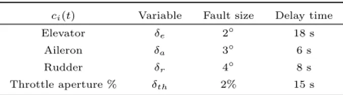
A suitable value of δ = 4 for the computation of the posi-tive and negaposi-tive thresholds in (14) has been considered, in order to minimise the false–alarm occurrence and to max-imise the fault sensitivity. To summarise the performances of the PM FDI scheme, the minimal detectable step faults on the various input sensors are collected in Table 1.

Table 1 PM diagnosis technique: minimal detectable step input sensor faults with δ = 4

ci(t) Variable Fault size Delay time

Elevator δe 2◦ 18 s

Aileron δa 3◦ 6 s

Rudder δr 4◦ 8 s

Throttle aperture % δth 2% 15 s

As to the NLGA, the synthesis of the residual genera-tors has been performed by using filter gains that optimise the fault sensitivity and reduce as much as possible the oc-currence of false alarms due to model uncertainties and to disturbances not completely decoupled.

In order to assess the NLGA diagnosis technique, in a similar way to PM evaluation, single step faults have been used. Moreover, also in this case the threshold values have been experimentally chosen according to (14).

A suitable value of δ = 8 for the computation of the pos-itive and negative thresholds in (14) has been considered. For what that concern NLGA FDI scheme, the minimal detectable step faults on the various input sensors are sum-marised in Table 2.

Table 2 NLGA diagnosis technique: minimal detectable step input sensor faults with δ = 8

ci(t) Variable Fault Size Delay Time

Elevator δe 2◦ 5 s

Aileron δa 2◦ 3 s

Rudder δr 2◦ 6 s

Throttle aperture % δth 6% 3 s

The minimal detectable fault values in Tables 1 and 2 are expressed in the unit of measure of the sensor signals. The

fault sizes are relative to the case in which the occurrence of a fault is detected and isolated as soon as possible. The detection delay times represent the worst case results. They are evaluated on the basis of the time taken by the slowest residual function to cross the settled threshold.

In the following, the robustness characteristic of the pro-posed PM and NLGA FDI schemes have been evaluated and compared to:

1) the unknown input Kalman filters (UIKF) scheme[1]

2) the neural networks (NN) technique[7]_.

The comparison tests have been performed with the same aircraft trajectory and based on the minimal detectable faults. In [11], with reference to a single straight flight condition, the different FDI schemes were approximately equally able to detect the sensor faults. On the other hand, the robustness property were not investigated.

In the remainder of this section, the performances of the different FDI schemes are evaluated by considering a more complex aircraft trajectory, depicted in Fig. 1. The shown trajectory has been obtained by means of the guidance and control functions of a standard autopilot, which stabilises the aircraft motion towards the reference trajectory being made up of the following 4 steady–state flight conditions:

1) 1st_{flight condition: true–air–speed = 50 (m/s); radius}

of curvature = ∞; flight–path angle = 0◦_{; altitude = 330} (m); flap deflection = 0◦

2) 2nd_{flight condition: true–air–speed = 50 (m/s); radius}

of curvature = 1000 (m); flight–path angle = 0◦_{; altitude} = 330 (m); flap deflection = 0◦_.

3) 3rd_{flight condition: true–air–speed = 50 (m/s); radius}

of curvature = ∞; flight–path angle = 0◦_{; altitude = 330} (m); flap deflection = 0◦_.

4) 4th_{flight condition: true–air–speed = 50 (m/s); radius}

of curvature = 1000 (m); flight–path angle = 0◦_{; altitude} = 330 (m); flap deflection = 0◦_.

Fig. 1 Aircraft 2D complete trajectory considered for the FDI scheme reliability evaluation

Note that both the 2nd _{and the 4}th _{reference flight}

con-ditions are equal to that one used to design the PM and the NLGA filters gave rise to the results of Tables 1 and 2, respectively. The performed tests represent a reliability evaluation of the considered FDI techniques. In fact, in this case the diagnosis requires that the residual generators be robust with respect to flight conditions not matching with

the nominal one which was adopted for the design. As an example, Fig. 2 shows the 4 residual functions gen-erated for the complete trajectory by the previously de-signed PM filter bank, which provided the results of Table 4 in the nominal flight condition. On the basis of the fault– free and faulty conditions represented in Fig. 2, this bank provides the correct isolation of the considered input sensor fault.

Fig. 2 PM residuals for the 1st_{input sensor fault f}

c1(t)

isolation with δ = 4

In particular, Fig. 2 represents the fault–free and the faulty residual signals. Horizontal lines show the levels of the fault–free thresholds that are settled according to test (14) with δ = 4. In the considered case, the fault has been generated on the 1st_{input sensor of the considered aircraft,}

starting at time t = 60 s. The first residual function, as depicted in Fig. 2, provides also the isolation of the fault

fc(t) regarding the 1stinput sensor. In fact the residual for the the 1st _{input does not depend on the considered fault,}

since it has been designed to be insensitive to the related input signal.

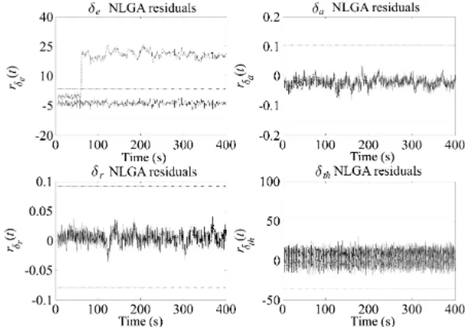
Fig. 3 NLGA residuals for the 1st_{input sensor fault isolation}

with δ = 12

The second example applied to the complete aircraft tra-jectory concerns with the 4 residual functions, shown in Fig. 3, generated by the NLGA filter bank whose results in the nominal flight condition are collected in Table 4. In Fig. 3, horizontal lines represent the thresholds of (14) with

δ = 12. Note that, due to the NLGA design technique

pre-sented in Section 3, only the 1st_{residual related to the δ} e signal of the filter bank is sensitive to a fault affecting the 1st_{input sensor.}

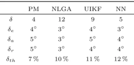
Table 3 summarises the results obtained by considering the observers and filters (corresponding to the PM, NLGA, UIKF and NN) for the input sensor FDI, whose parameters have been designed and optimised for the steady–state co-ordinated turn being represented by the 2nd_{reference flight}

condition of the complete trajectory. In Table 3, the per-formances of the considered FDI techniques in terms of the minimal detectable step faults on the various input sen-sors are reported, as well as the corresponding parameters

δ for the residual evaluation (14). The choice of δ has been

performed with reference to the particular flight conditions involved in the complete trajectory following. In particu-lar, the selected value of δ for each FDI observer or filter represents a trade–off between two objectives:

1) to increase as much as possible the residual fault sen-sitivity and promptness

2) to minimise the occurrence of false–alarms due to the switching among the reference flight conditions needed to stabilise the aircraft motion towards the reference trajec-tory.

Table 3 Reliability analysis of the FDI schemes for a complete aircraft trajectory PM NLGA UIKF NN δ 4 12 9 5 δe 4◦ 3◦ 4◦ 3◦ δa 5◦ 3◦ 5◦ 4◦ δr 5◦ 3◦ 4◦ 4◦ δth 7 % 10 % 11 % 12 %

Table 3 shows how the proper design of the parameter δ allows to obtain good performances with all the considered FDI schemes, hence the robustness with respect to the pro-posed complete trajectory is always achieved.

It is worth noting that the NLGA has a theoretical ad-vantage by taking into account the nonlinear dynamics of the aircraft. However, the behaviour of the related non-linear residual generators is quite sensitive to the model uncertainties. In fact, the NLGA FDI scheme requires high values of δ which have to be increased (from 8 to 12 in this work) when the aircraft motion regarding the complete trajectory is considered in place of the nominal flight con-dition. In particular, even though the analysis is restricted just to the aircraft turn phase of the complete trajectory, a performance degradation would happen, since the steady– state condition (nominal flight condition) is quite far to be reached. Anyway, the filter design based on the NLGA leads to a satisfactory fault detection, above all in terms of promptness. On the other hand, regarding the PM, it is rather simple to note the good FDI performances, even if optimisation stages may be required. The δ values selected for the PM are lower, but the related residual fault sensi-tivities are even smaller. Similar comments can be made for the UIKF and NN techniques.

The simulation model applied to the complete trajectory, depicted in Fig. 1, is an effective way to test the

perfor-mances of the proposed FDI methods with respect to mod-elling mismatch and measurement errors. The obtained re-sults demonstrate the reliability of the PM, NLGA, UIKF and NN based FDI schemes as long as proper design pro-cedures are adopted.

5

Conclusion

The paper provided a novel development and application of two FDI techniques based on a PM scheme and on a NLGA method, respectively. As to the PM, the FDI proce-dure led to residual generators optimising the trade–off be-tween robustness and fault sensitivity. As to the NLGA, the FDI procedure was applied for the first time to an aircraft model in flight conditions characterised by tight–coupled longitudinal and lateral dynamics. Moreover, the related application was robust to model uncertainties.

The PM and NLGA residual generators were tested by a PIPER PA30 simulator embedding the models of wind gusts, Dryden turbulence, sensors measurement errors, en-gine and servo actuators. Moreover, in order to verify the robustness characteristics and the achievable performances of the approaches, the simulation results adopted a typical aircraft reference trajectory embedding several steady–state flight conditions, such as straight flight phases and coordi-nated turns.

Finally, the effectiveness of the developed PM and NLGA FDI schemes was shown by simulations and a compari-son with widely used data–driven and model–based FDI schemes, such as NN and UIKF diagnosis methods. The comparison highlighted that the PM and NLGA FDI schemes have approximately the same performance of those related to NN and UIKF based schemes. In some case, it is possible to note a bit better performance of the PM and NLGA schemes. On the other hand, it is important to ob-serve that an advantage of PM and NLGA is the simplicity of the structure of the residual generators. This aspect high-lights the potential to use such methods also in real aircraft applications.

References

[1] J. Chen, R. J. Patton. Robust Model–Based Fault

Diag-nosis for Dynamic Systems. Kluwer Academic Publishers,

Boston, 1999.

[2] R. J. Patton, P. M. Frank, R. N. Clark. Issues of Fault

Diagnosis for Dynamic Systems. Springer–Verlag, London,

2000.

[3] S. Simani, C. Fantuzzi, R. J. Patton. Model-based Fault

Diagnosis in Dynamic Systems Using Identification Tech-niques. Springer–Verlag, London, 2002.

[4] R. Isermann. Fault–Diagnosis Systems: An Introduction

from Fault Detection to Fault Tolerance. Springer–Verlag,

Berlin, 2005.

[5] J. Gertler. Fault Detection and Diagnosis in Engineering

Systems. Marcel Dekker, New York, 1998.

[6] M. Basseville, I. V. Nikiforov. Detection of Abrupt Changes: Theory and Application. Prentice–Hall,

Engle-wood Cliffs, 1993.

[7] J. Korbicz, J. M. Koscielny, Z. Kowalczuk, W. Cholewa.

Fault Diagnosis: Models, Artificial Intelligence, Applica-tions. Springer–Verlag, Berlin, 2004.

[8] C. De Persis, A. Isidori. On the Observability Codistribu-tions of a Nonlinear System. Systems and Control Letters, vol. 40, no. 1, pp. 297–304, 2000.

[9] C. De Persis, A Isidori. A Geometric Approach to Non– linear Fault Detection and Isolation. IEEE Transactions

on Automatic Control, vol. 45, no. 6, pp. 853–865, 2001.

[10] C. De Persis, R. De Sanctis, A. Isidori. Nonlinear Actuator Fault Detection and Isolation for a VTOL Aircraft. In

Pro-ceedings of the American Control Conference, Arlington,

VA, USA, vol. 6, pp. 4449–4454, 2001.

[11] M. Bonf`e, P. Castaldi, W. Geri, S. Simani. Fault Detection and Isolation for On–board Sensors of a General Aviation Aircraft. International Journal of Adaptive Control and

Signal Processing, vol. 20, no. 8, pp. 381–408, 2006.

[12] B. L. Stevens, F. L. Lewis. Aircraft Control and Simulation. John Wiley and Son, New York, 2003.

Marcello. Bonf`e received his M.Sc. de-gree in electronic engineering from the Uni-versity of Ferrara, Italy, in 1998, and the Ph.D. degree in information engineering from the University of Modena and Reggio Emilia, Italy, in 2003. Currently, he is an assistant professor in automatic control at the Department of Engineering of the Uni-versity of Ferrara, Italy.

He has published about 30 refereed jour-nal and conference papers. His current research interests include fault detection and isolation, modelling and control of mecha-tronic systems and formal verification methods for discrete event systems.

Paolo Castaldi received his Laurea de-gree (cum laude) in electronic engineering in 1990 from the University of Bologna and the Ph.D degree in system engineering in 1994, both from the University of Bologna, Padova and Firenze. Since 1995 he has been assistant professor at the Department of Electronics, Computer Science and Sys-tems of the University of Bologna.

He has published more than 70 refereed journal and conference papers. His research interests include fault diagnosis, adaptive filtering, system identification, and their applications to aerospace and mechanical systems.

Prof. Castaldi is a reviewer of many international journals. He was awarded as “outstanding reviewer” of Automatica in 2004 and 2005.

Walter Geri received his Laurea de-gree (cum laude) in computer science en-gineering from the University of Bologna, Italy, in 2001 and the Ph.D. degree in system engineering from the University of Bologna, in 2005. Since 2005 he was re-search fellow at the University of Bologna. Since 2006 he has held a course of “Auto-matic Control System Design” at the 2nd

Faculty of Engineering of the University of Bologna.

He has published more than 20 refereed journal and confer-ence papers. His research interests include fault diagnosis, adap-tive filtering, guidance algorithms, satellite–based navigation and their applications to aerospace systems.

Silvio Simani received his Laurea degree (cum laude) in electrical engineering from the Department of Engineering at the Uni-versit`a degli Studi di Ferrara, Italy, in 1996 and the Ph.D. degree in information sci-ence: automatic control at the Department of Engineering of the University of Ferrara and Modena, Italy, in 2000. Since February 2002 he has been assistant professor at the Department of Engineering of the Univer-sity of Ferrara.

He has published about 90 refereed journal and conference pa-pers and one book. His research interests include fault diagnosis of dynamic processes, system modelling and identification, and the interaction issues between identification and fault diagnosis. Prof. Simanniis a reviewer of many international journals. He is IEEE senior member, and member of the Technical Committee SAFEPROCESS.