CLASH: THE CONCENTRATION-MASS RELATION OF GALAXY CLUSTERS
J. Merten1,2,3, M. Meneghetti1,4,5, M. Postman6, K. Umetsu7, A. Zitrin2,32, E. Medezinski8, M. Nonino9, A. Koekemoer6, P. Melchior10, D. Gruen11,12, L. A. Moustakas1, M. Bartelmann13, O. Host14, M. Donahue15, D. Coe6, A. Molino16, S. Jouvel17,18, A. Monna11,12, S. Seitz11,12, N. Czakon7, D. Lemze8, J. Sayers2, I. Balestra9,19, P. Rosati20, N. Benítez15,
A. Biviano9, R. Bouwens21, L. Bradley6, T. Broadhurst22,23, M. Carrasco13,24, H. Ford8, C. Grillo14, L. Infante25, D. Kelson26, O. Lahav17, R. Massey27, J. Moustakas28, E. Rasia29, J. Rhodes1,2, J. Vega30,31, and W. Zheng6
1
Jet Propulsion Laboratory, California Institute of Technology, 4800 Oak Grove Drive, Pasadena, CA 91109, USA;[email protected]
2
California Institute of Technology, MC 249-17, Pasadena, CA 91125, USA 3
Department of Physics, University of Oxford, Keble Road, Oxford OX1 3RH, UK 4
INAF, Osservatorio Astronomico di Bologna, via Ranzani 1, I-40127 Bologna, Italy 5
INFN, Sezione di Bologna, Viale Berti Pichat 6/2, I-40127 Bologna, Italy 6
Space Telescope Science Institute, 3700 San Martin Drive, Baltimore, MD 21208, USA 7
Institute of Astronomy and Astrophysics, Academia Sinica, P.O. Box 23-141, Taipei 10617, Taiwan 8
Department of Physics and Astronomy, The Johns Hopkins University, 3400 North Charles Street, Baltimore, MD 21218, USA 9
INAF/Osservatorio Astronomico di Trieste, via G.B. Tiepolo 11, I-34143 Trieste, Italy 10
Center for Cosmology and Astro-Particle Physics and Department of Physics, The Ohio State University, Columbus, OH 43210, USA 11
Universitäts-Sternwarte München, Scheinerstr. 1, D-81679 München, Germany 12
Max-Planck-Institute für extraterrestrische Physik, Giessenbachstr. 1, D-85748 Garching, Germany 13
Universität Heidelberg, Zentrum für Astronomie, Institut für Theoretische Astrophysik, Philosophenweg 12, D-69120 Heidelberg, Germany 14
Dark Cosmology Centre, Niels Bohr Institute, University of Copenhagen, Juliane Maries Vej 30, DK-2100 Copenhagen, Denmark 15
Department of Physics and Astronomy, Michigan State University, East Lansing, MI 48824, USA 16
Instituto de Astrofísica de Andalucía(CSIC), E-18080 Granada, Spain 17Institut de Ciéncies de l’Espai (IEEC-CSIC), E-08193 Bellaterra (Barcelona), Spain 18
Department of Physics and Astronomy, University College London, London WC1E 6BT, UK 19INAF—Osservatorio Astronomico di Capodimonte, Via Moiariello 16, I-80131 Napoli, Italy 20
Dipartimento di Fisica e Scienze della Terra, Università degli Studi di Ferrara, Via Saragat 1, I-44122 Ferrara, Italy 21
Leiden Observatory, Leiden University, P. O. Box 9513, NL-2333 Leiden, The Netherlands 22
Department of Theoretical Physics and History of Science, University of the Basque Country UPV/EHU, P.O. Box 644, E-48080 Bilbao, Spain 23
Ikerbasque, Basque Foundation for Science, Alameda Urquijo, 36-5 Plaza Bizkaia, E-48011 Bilbao, Spain 24
Instituto de Astrofsica, Facultad de Física, Pontificia Universidad Católica de Chile, Casilla 306, Santiago 22, Chile 25
Centro de Astro-Ingeniería, Departamento de Astronomía y Astrofísica, Pontificia Universidad Catolica de Chile, V. Mackenna 4860, Santiago, Chile 26
Observatories of the Carnegie Institution of Washington, Pasadena, CA 91101, USA 27
Institute for Computational Cosmology, Durham University, South Road, Durham DH1 3LE, UK 28
Department of Physics and Astronomy, Siena College, 515 Loudon Road, Loudonville, NY 12211, USA 29
Physics Dept., University of Michigan, 450 Church Ave, Ann Arbor, MI 48109, USA 30
Departamento de Física Teórica, Universidad Autónoma de Madrid, Cantoblanco, E-28049 Madrid, Spain 31
LERMA, CNRS UMR 8112, Observatoire de Paris, 61 Avenue de l’Observatoire, F-75014 Paris, France Received 2014 April 8; accepted 2015 April 2; published 2015 June 3
ABSTRACT
We present a new determination of the concentration–mass (c–M) relation for galaxy clusters based on our comprehensive lensing analysis of 19 X-ray selected galaxy clusters from the Cluster Lensing and Supernova Survey with Hubble (CLASH). Our sample spans a redshift range between 0.19 and 0.89. We combine weak-lensing constraints from the Hubble Space Telescope(HST) and from ground-based wide-field data with strong lensing constraints from HST. The results are reconstructions of the surface-mass density for all CLASH clusters on multi-scale grids. Our derivation of Navarro–Frenk–White parameters yields virial masses between
M h
0.53×10¹⁵
⊙ and1.76×1015M⊙ h and the halo concentrations are distributed around c200c∼3.7 with a
1σ significant negative slope with cluster mass. We find an excellent 4% agreement in the median ratio of our measured concentrations for each cluster and the respective expectation from numerical simulations after accounting for the CLASH selection function based on X-ray morphology. The simulations are analyzed in two dimensions to account for possible biases in the lensing reconstructions due to projection effects. The theoretical c– M relation from our X-ray selected set of simulated clusters and the c–M relation derived directly from the CLASH data agree at the 90% confidence level.
Key words: dark matter– galaxies: clusters: general – gravitational lensing: strong – gravitational lensing: weak 1. INTRODUCTION
The standard model of cosmology (ΛCDM) is extremely successful in explaining the observed large-scale structure of the universe (see, e.g., Anderson et al. 2012; Planck Collaboration et al. 2014). However, when moving to progressively smaller length scales, inconsistencies between
theoretical predictions and real observations have emerged. Examples include the cored mass-density profiles of dwarf-spheroidal galaxies (Walker & Peñarrubia 2011), the abun-dance of Milky Way satellites (Boylan-Kolchin et al. 2012), and theflat dark matter density profiles in the cores of galaxy clusters(Sand et al.2002; Newman et al.2013).
Galaxy clusters are unique tracers of cosmological structure formation(e.g., Voit2005; Borgani & Kravtsov2011). As the © 2015. The American Astronomical Society. All rights reserved.
32
largest collapsed objects in the observable universe, clusters form the bridge between the large-scale structure of the universe and the astrophysical regime of individual halos. From an observational point of view, all main mass components of a cluster, hot ionized gas, dark matter, and luminous stars, are directly or indirectly observable with the help of X-ray observatories (e.g., Rosati et al. 2002; Ettori et al. 2013), gravitational lensing (e.g., Bartelmann & Schneider 2001; Bartelmann2010), or optical observations.
As shown by numerical simulations (Navarro et al. 1996), dark matter tends to arrange itself following a specific, spherically symmetric density profile
(
)
r r r r r ( ) 1 , (1) s s s NFW 2 ρ = ρ +where the only two parametersρ and rs sare a scale density and
a scale radius. This functional form is now commonly called the Navarro–Frenk–White (NFW) density profile. It was found to fit well the dark matter distribution of halos in numerical simulations, independent of halo mass, cosmological para-meters, or formation time (Navarro et al. 1997; Bullock et al.2001).
A specific parametrization of the NFW profile uses the total mass enclosed within a certain radius rΔ
(
)
M π r c c c 4 ln 1 1 , (2) s s 3 ρ = + − + Δ Δ Δ Δ ⎛ ⎝ ⎜ ⎞ ⎠ ⎟ and the concentration parameterc r
rs. (3)
=
Δ Δ
When applying the relations above to a specific analysis, the radius rΔis chosen such that it describes the halo on the scale of
interest. An example is the radius at which the average density of the halo is 200 times the critical density of the universe at this redshift (Δ =200c). Cosmological simulations show that there is a correlation between mass and concentration for dark matter structures, although with significant scatter. This defines the concentration–mass (c–M) relation which is a mild function of formation redshift and halo mass(Bullock et al.2001; Eke et al.2001; Zhao et al.2003; Duffy et al.2008; Gao et al.2008; Klypin et al.2011; Prada et al.2012; Bhattacharya et al.2013). Observational efforts have been undertaken to measure the c–M relation either using gravitational lensing (Comerford & Natarajan 2007; Oguri et al.2012; Okabe et al. 2013), X-ray observations(Buote et al.2007; Schmidt & Allen2007; Ettori et al.2010), or dynamical analysis of cluster members (Lemze et al.2009; Wojtak &Łokas2010; Biviano et al.2013). Some of the observed relations are in tension with the predictions of numerical simulations (Duffy et al. 2008; Fedeli 2012). The most prominent example of such tension is the cluster Abell 1689(Broadhurst et al.2005; Peng et al.2009, and references therein), with a concentration parameter up to a factor of three higher than predicted. In a follow-up study, Broadhurst et al. (2008) compared a larger sample of five clusters to the prediction fromΛCDM and found the derived c–M relation in tension with the theoretical expectations (see also Broadhurst & Barkana 2008a; Zitrin et al.2010; Meneghetti et al.2011). Possible explanations for these discrepancies include a selection-bias of the cluster sample since these clusters were
known strong lenses, paired with the assumption of spherical symmetry for these systems(Hennawi et al.2007; Meneghetti et al.2010a). Moreover, the influence of baryons on the cluster core(Fedeli2012; Killedar et al.2012) and even the effects of early dark energy (Fedeli & Bartelmann 2007; Sadeh & Rephaeli2008; Francis et al. 2009; Grossi & Springel 2009) have been introduced as possible explanations. Ultimately, a new set of high-quality observations of an unbiased ensemble of clusters was needed to answer the question if observed galaxy clusters are indeed in tension with our cosmological standard model.
The Cluster Lensing And Supernova Survey with Hubble (CLASH; Postman et al. 2012a) is a multi-cycle treasury program, using 524 Hubble Space Telescope (HST) orbits to target 25 galaxy clusters, largely drawn from the Abell and MACS cluster catalogs(Abell1958; Abell et al.1989; Ebeling et al. 2001, 2007, 2010). Twenty clusters were specifically selected by their largely unperturbed X-ray morphology with the goal of representing a sample of clusters with regular, unbiased density profiles that allow for an optimal comparison to models of cosmological structure formation. As reported in Postman et al.(2012a) all clusters of the sample are fairly X-ray luminous with X-X-ray temperatures Tx⩾5keV and show a smooth morphology in their X-ray surface brightness. For all systems the separation between the brightest cluster galaxy (BCG) and the X-ray luminosity centroid is 20< kpc. An overview of the basic properties of the sample can be found in Table 1. In the following we will use these X-ray selected clusters to derive the observed c–M relation for CLASH clusters based on weak and strong lensing and perform a thorough comparison to the theoretical expectation from numerical simulations. This study has two companion papers. The weak-lensing and magnification analysis of CLASH clusters by Umetsu et al.(2014) and the detailed characteriza-tion of numerical simulacharacteriza-tions of CLASH clusters by Mene-ghetti et al.(2014).
This paper is structured as follows. Section 2 provides a basic introduction to gravitational lensing and introduces the method used to recover the dark matter distribution from the observational data. The respective input data is described in Section3 and the resulting mass maps and density profiles of the CLASH clusters are presented in Section 4. We interpret our results by a detailed comparison to theoretical c–M relations from the literature in Section 5 and use our own tailored set of simulations to derive a CLASH-like c–M relation in Section6. We conclude in Section7. Throughout this work we assume a flat cosmological model similar to a WMAP7 cosmology(Komatsu et al.2011) withW =m 0.27,W =Λ 0.73,
and a Hubble constant of h=0.7. For the redshift range of our cluster sample this translates to physical distance scales of 3.156–7.897 kpc/″.
2. CLUSTER MASS PROFILES FROM GRAVITATIONAL LENSING
We use gravitational lensing to recover the distribution of matter in galaxy clusters from imaging data. Lensing is particularly well-suited for this purpose since it is sensitive to the lens’ total matter content, independent of its composition and under a minimum number of assumptions. After we discussed the basics of this powerful technique we will present a non-parametric inversion algorithm which maps the dark matter mass distribution over a wide range of angular scales.
The CLASH data were designed to provide a unique combination of angular resolution, depth and multi-wavelength coverage that allows many new multiply lensed galaxies to be identified and their redshifts to be accurately estimated. These data are ideal for use with the SaWLens algorithm, which makes no a priori assumptions about the distribution of matter in a galaxy cluster.
2.1. Gravitational Lensing
Gravitational lensing is a direct consequence of Einsteinʼs theory of general relativity (see, e.g., Bartelmann 2010, for a complete derivation). For cluster-sized lenses the lens mapping can be described by the lens equation
( ). (4)
β =θ−α θ
This lens equation describes how the original 2D angular position in the source plane β =( ,β β1 2) is shifted by a deflection angle α= ( ,α α1 2) to the angular coordinates
( ,1 2)
θ = θ θ in the lens plane. From now on we denote the angular diameter distance between observer and lens as Dl,
between observer and source as Ds, and between lens and
source as Dls. The deflection angle depends on the
surface-mass density distribution of the lensΣ(Ddθ)and can be related to a lensing potential
(
)
π d D ( ) : 1 2 l ln , (5) cr∫
θ θ θ θ ψ = θ′Σ Σ − ′which is a line of sight projected and rescaled version of the Newtonian potential. The cosmological background model enters this equation through the critical surface mass density for
lensing given by c πG D D D 4 , (6) cr 2 l s ls Σ =
where c is the speed of light and G is Newtonʼs constant. By introducing the complex lensing operators (e.g., Bacon et al. 2006; Schneider & Er 2008) : i
1 2 θ θ ∂ = ∂ ∂ + ∂ ∂ ⎛ ⎝ ⎜ ⎞ ⎠ ⎟ and i * : 1 2 θ θ ∂ = ∂ ∂ − ∂ ∂ ⎛ ⎝ ⎜ ⎞ ⎠
⎟ one can derive important lensing quan-tities as derivatives of the lensing potential
s s s : 1 2 : 2 2 : * 0 (7) α ψ γ ψ κ ψ = ∂ = = ∂∂ = = ∂∂ =
whereα is the complex form of the already known deflection angle,γ is called the complex shear, and the scalar quantity κ is called convergence. The behavior of each quantity under rotations of the coordinate frame is given by the spin-parameter s.
When relating these basic lens quantities to observables one distinguishes two specific regimes. In the case of weak lensing the distortions induced by the lens mapping are small and due to the intrinsic ellipticity of galaxies, localized averages over an ensemble of sources are used to separate the lensing signal from the random orientation caused by the intrinsic ellipticity. These local averages of ellipticity measurements can be related to Equation(7) by the reduced shear g
g : 1 , (8) γ κ = = − Table 1
The CLASH X-Ray Selected Cluster Sample
Name z R.A. Decl. k Txa Lbola ″→ kpcb
(deg/J2000) (deg/J2000) (keV) (1044erg s−1)
Abell 383 0.188 42.014090 −3.5292641 6.5 6.7 3.156 Abell 209 0.206 22.968952 −13.611272 7.3 12.7 3.392 Abell 1423 0.213 179.32234 33.610973 7.1 7.8 3.482 Abell 2261 0.225 260.61336 32.132465 7.6 18.0 3.632 RX J2129+0005 0.234 322.41649 0.0892232 5.8 11.4 3.742 Abell 611 0.288 120.23674 36.056565 7.9 11.7 4.357 MS 2137−2353 0.313 325.06313 −23.661136 5.9 9.9 4.617 RXC J2248−4431 0.348 342.18322 −44.530908 12.4 69.5 4.959 MACS J1115+0129 0.352 168.96627 1.4986116 8.0 21.1 4.996 MACS J1931−26 0.352 292.95608 −26.575857 6.7 20.9 4.996 RX J1532.8+3021 0.363 233.22410 30.349844 5.5 20.5 4.931 MACS J1720+3536 0.391 260.06980 35.607266 6.6 13.3 5.343 MACS J0429−02 0.399 67.400028 −2.8852066 6.0 11.2 5.411 MACS J1206−08 0.439 181.55065 −8.8009395 10.8 43.0 5.732 MACS J0329−02 0.450 52.423199 −2.1962279 8.0 17.0 5.815 RX J1347−1145 0.451 206.87756 −11.752610 15.5 90.8 5.822 MACS J1311−03 0.494 197.75751 −3.1777029 5.9 9.4 6.128 MACS J1423+24 0.545 215.94949 24.078459 6.5 14.5 6.455 MACS J0744+39 0.686 116.22000 39.457408 8.9 29.1 7.186 CL J1226+3332 0.890 186.74270 33.546834 13.8 34.4 7.897 a
From Postman et al.(2012a) and references therein.
b
where we defined the ellipticity of a galaxy as a b a b : ∣ ∣ = − +
with the two axes of the ellipse fulfilling a> . This relationb between the measured ellipticities and the properties applies only in the regime where g∣ ∣ <1and assumes that the shear is constant across a galaxy (Schneider & Er 2008). To mitigate this, we exclude shear measurements inside the region where
g 1
∣ ∣ > (see also Section3.2). For the combination of galaxy shape moments used in the RRG method, the constant shear approximation remains correct (to within 1% for a singular isothermal sphere lens) outside 1.07 times the Einstein radius (Massey & Goldberg2008). This potential source of bias is far smaller than other sources of statistical error in our current analysis. For completeness we note that for g∣ ∣ > , the relation1 between the measured ellipticities and the properties of the lens switches to 1 * . (9) κ γ = −
For a more thorough description of the relation between the measured shapes of galaxy images and the lens properties in the weak lensing regime we refer to the review by(Bartelmann & Schneider 2001, and references therein). We also do not discuss here the many systematic effects to be taken into account during such a shape measurement but refer to, e.g., Kitching et al.(2012), Massey et al. (2013), or Mandelbaum et al.(2014).
In the strong lensing regime, close to the core of the lens’ mass distribution, the assumption of small image distortions does not hold any more. The lens equation becomes nonlinear and therefore multiple images of the same source can form. This happens near the critical line at a given redshift which is defined by the roots of the lensing Jacobian
det=(1−κ)2 −γ2. (10)
While the weak lensing regime expands over the full cluster field, it does not describe the mass distribution in the center of the cluster. Strong lensing is limited to the inner-most 10″–50″ of the cluster field, which renders the combination of the two regimes the ideal approach for mass reconstruction. One particular limitation of gravitational is the mass-sheet-degen-eracy (Falco et al.1985; Gorenstein et al. 1988). It describes the invariance of many lensing observables under the transformation
( )θ ( )θ ( )θ (1 ) (11)
κ → ′κ =λκ + −λ
( )θ ( )θ ( )θ (12)
γ → ′γ =λγ
with the free33transformation parameterλ. Several ways have been suggested to break the mass-sheet-degeneracy, including the use of magnification constraints (e.g., Broadhurst et al. 1995), which are not invariant under the mass-sheet transformation, and the inclusion of multi-redshift strong-lensing features (Bradač et al. 2004, 2005b). In this work, however, we will folow another route to break the mass-sheet-degeneracy, which is the simple condition that the average
convergence at the edge of the reconstructionfield goes to zero in the absence of a lensing signal. This assumption is justified once wide-field imaging is used, entailing the full cluster field well-beyond its virial radius and we will present its specific implementation into our reconstruction algorithm in the next section.
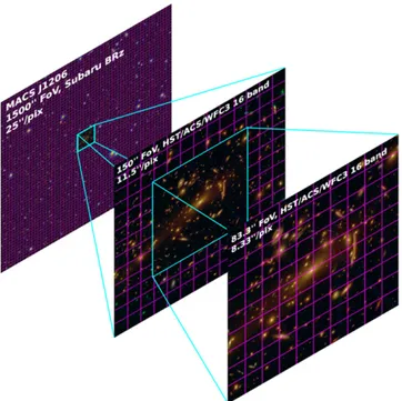
2.2. Non-parametric Lensing Inversion WithSaWLens The SaWLens (Strong -and Weak-lensing) method was developed with two goals in mind. First, it should consistently combine weak and strong lensing. The second goal was to make no a priori assumptions about the underlying mass distribution, but to build solely upon the input data. The initial idea for such a reconstruction algorithm was formulated by Bartelmann et al. (1996) and was further developed by Seitz et al. (1998) and Cacciato et al. (2006). Similar ideas were implemented by Bradač et al. (2005b) with first applications to observations in Bradač et al. (2005a, 2006). Other non-parametric reconstruction algorithms, based on different methdologies, have been presented by Abdelsalam et al. (1998), Bridle et al. (1998), Liesenborgs et al. (2006), Jee et al. (2007), Diego et al. (2007), and Merten (2014). In its current implementation (Merten et al. 2009), SaWLens performs a reconstruction of the lensing potential (Equation (5)) on an adaptively refined grid. In this particular study, the method uses three different grid sizes to account for weak lensing on a widefield, such as is provided by ground-based telescopes, weak lensing constraints from the HST on a much smaller field of view but with considerably higher spatial resolution, and a fine grained grid to trace strong lensing features near the inner-most core of the cluster. This three-level adaptive grid is illustrated in Figure1.
Figure 1. Visualization of our multi-scale approach. While weak lensing data from Subaru allows for a mass reconstruction of a galaxy cluster on a wide field, the achievable resolution is rather low. HST weak lensing delivers higher resolution but on a relatively smallfield. Finally, the strong lensing regime provides a very high resolution, but only in the inner-most cluster core. This figure shows one of our sample clusters, MACS J1206 and the reconstruction grids for all three lensing regimes.
33
The parameter is free up to the limit that the solution for the surface-mass density must be physical in terms of e.g., the dynamics of cluster member galaxies etc.
SaWLens uses a statistical approach to reconstruct the lensing potential ψ in every pixel of the grid. A χ2-function,
which depends on the lensing potential and includes a weak and a strong-lensing term is defined by
( ) w( ) s ( ), (13)
2 2 2
χ ψ =χ ψ +χ ψ
and the algorithm minimizes it such that the input data is best described by a pixelized lensing potentialψl
( ) 0. (14) l 2 ! χ ψ ψ ∂ ∂ =
In Equation(14), l runs over all grid pixels. The weak-lensing term in Equation (13) is derived from Equation (8) with a measured average complex ellipticity of background sources in each grid pixel ϵ
g g ( ( )) ( ( )) . (15) i j i ij j 2 , 1 w
∑
χ = ε− ψ − ε− ψThe covariance matrix is non-diagonal because the algorithm adaptively averages over a number of background-ellipticity measurements in each pixel to account for the intrinsic ellipticity of background sources. Depending on the recon-struction resolution, this number is either defined by all weak-lensing background galaxies that are contained within the area of the current reconstruction pixel, or, if the reconstruction resolution is high, the algorithm searches in progressively larger squares around the center of the reconstruction pixel until at least 10 galaxies are contained in the square area. Due to this averaging scheme, neighboring pixels may share a certain number of background sources and the algorithm keeps track of these correlations between pixels as described in Section3.2and especially Equations (14)–(16) of Merten et al. (2009). We do not perform any distance-weighting in our averages since we treat our reconstruction cells as extended square pixels. However, during the averaging process each measured ellipticity is weighted with the inverse-variance of the shape measurement. This approach has been calibrated and is tested by reconstructing numerically simulated lenses in Merten et al. (2009) and Meneghetti et al. (2010b). The connection to the lensing potential is given by Equation (8) which, when inserted into Equation (15), yields
Z z Z z Z z Z z ( ) ( ) ( ) 1 ( ) ( ) ( ) ( ) 1 ( ) ( ) , (16) i j i ij j 2 , 1 w
∑
χ ψ ε γ ψ κ ψ ε γ ψ κ ψ = − − × − − − ⎛ ⎝ ⎜ ⎞⎠⎟ ⎛ ⎝ ⎜ ⎞⎠⎟where again both indices i and j run over all grid cells. Note that all lensing quantities given by Equation(7) have a redshift dependence introduced by the critical density in Equations(5) and (6). This is taken into account by a cosmological weight function(Bartelmann & Schneider2001) scaling each pixel to afiducial redshift of infinity during the reconstruction.
Z z D D D D H z z ( ) : ls ( ). (17) l s l = ∞ − ∞
The Heaviside step function ensures that only sources behind the lens redshift zl have non-zero weight.
The definition of the strong lensing term in Equation (13) makes use of the fact the position of the lens’ critical line at a certain redshift can be inferred from the position of multiple images. It has been shown in Merten et al. (2009) and Meneghetti et al.(2010b) that pixel sizes 5> ″ are large enough to make this simple assumption. Therefore, following Equation (10) Z z Z z ( ) det ( ) (1 ( ) ( )) ( ) ( ) , (18) i i i i 2 2 , 2 2 2 2 , 2 s s s χ ψ ψ σ κ ψ γ ψ σ = = − −
where this term is only assigned to those grid cells which are part of the critical line at a certain redshift z given the positions of multiple images. The error termσ is then given by the cell size of the grid following
det , (19) s E c σ θ δθ δθ θ ≈ ∂ ∂ θ ≈
withθ being an estimate of the Einstein radius of the lens.E
The missing connection to the lensing potentialψ is given by Equation(7). The numerical technique of finite differencing is then used to express the basic lensing quantities by simple matrix multiplications (20) i ij j κ = ψ (21) i ij j 1 1 γ = ψ (22) i ij j 2 2 γ = ψ where ij, ij 1 , and ij 2
are sparse matrices representing the finite differencing stamp of the respective differential operator (Seitz et al. 1998; Bradač et al. 2005a; Merten et al. 2009). With these identities in mind it can be shown that Equation (14) takes the form of a linear system of equations, which is solved numerically. There are two important aspects to this method, which we will only mention briefly. First, a two-level iteration scheme is employed to deal with the nonlinear nature of the reduced shear(Schneider & Seitz 1995) and to avoid overfitting of local noise contributions (Merten et al. 2009). Second, a regularization scheme is adapted(Seitz et al. 1998; van Waerbeke 2000) to ensure a smooth transition from one iteration step to the next. In this work we adapt the regularization scheme of Bradač et al. (2005a), with an initial flat convergence prior, which regularizes the initial conver-gence to zero over thefield. This also conveniently implements the way in which we break the mass-sheet-degeneracy, as we have mentioned earlier on. The initial regularization condition ensures aflat and zero convergence field where no significant lensing signal is found in the shear data.
It is important that a complex lensing inversion algorithm is tested thoroughly and under controlled but realistic conditions. Such tests are particular importance for our analysis since we are applying our method to a large set of real clusters of galaxies and we need to know our expected level of systematic error in the determination of masses and concentrations. Also,
we use several techniques which rely on specific assumptions and hence need to be tested for their validity. This includes our way of breaking the mass-sheet degeneracy, the use of critical line estimators in the strong-lensing regime and the two-level iteration with a specific regularization scheme.
These tests were performed in Meneghetti et al. (2010b) with a set of three simulated clusters with masses between 6.8×10¹⁴–1.1×10¹⁵M h
⊙ . Each of the three simluated
clusters was reconstructed in three perpendicular projections, spanning a range of surface-mass densities of fairly round, to elliptical and highly substuctured morphologies. Figure 15 of Meneghetti et al.(2010b) shows that SaWLens determines the masses of this particular set of simulations with an accuracy of 5%–10% at all relevant radii. Other methods relying on either strong -or weak-lensing constraints are limited to either small or large scales and showed less accurate results with errors of ∼20%. SaWLens also recovered the concentrations of the simulated halos with errors at the∼5% level. These results on concentrations are summarized in Table 3 of Meneghetti et al. (2010b). We want to emphasize that the quoted errors refer to the results when reconstructing a set of nine projections from three cluster simulations. This number is smaller than the 19 cluster reconstructions shown in this work and the simulated cluster sample was also not explicitly constructed to mimick the CLASH selection. Hence, these tests can only serve as an approximate lead for the accuracy of individual cluster reconstructions of this work, but nevertheless represent an important check of our methodlogy and numerical implemen-tation. Aside from the successful tests on simulated lenses, the SaWLens algorithm has been used in the reconstruction of observed galaxy clusters (Merten et al. 2009, 2011; Umetsu et al.2012; Medezinski et al.2013; Patel et al.2014).
3. THE CLASH DATA SET
Our analysis focuses on the X-ray selected sub-sample of CLASH(Table1). For each of these clusters a large number of lensing constraints was collected, either from the HST CLASH survey (Postman et al. 2012a), the accompanying Subaru/ Suprime-Cam (Umetsu et al. 2011; Postman et al. 2012a; Medezinski et al.2013) or ESO/WFI (Gruen et al.2013) weak lensing observations, or from the CLASH-Very Large Tele-scope(VLT) spectroscopic program (Balestra et al.2013). The data collection includes strong-lensing multiply imaged systems together with accurate spectroscopic or photometric redshifts and weak-lensing shear catalogs on the full cluster field, paired with a reliable background selection of weak lensing sources.
3.1. Strong Lensing in the HST Fields
The Zitrin et al. (2009) method is applied to identify multiple-image systems in each cluster field. The respective strong-lensing mass models for several CLASH clusters have already been published(Zitrin et al.2011,2012a,2012b,2013; Coe et al.2012,2013; Umetsu et al.2012; Zheng et al.2012) and the full set of strong-lensing models and multiple-image identifications is presented in Zitrin et al. (2014). Exceptions are the cluster RXC J2248, where the multiple-image identi fi-cation is based on the Monna et al.(2014) strong-lensing mass model, and RX J1532, where our team was not able to identify any strong-lensing features to date. In this case, we derive the underlying lensing potential from weak lensing only with a
significantly coarser resolution in the central region, compared to the strong-lensing clusters.
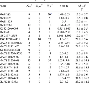
A summary of multiple-image systems found in each cluster is given in Table 2. From the identified multiple images we estimate the locations of critical lines following the approach of Merten et al.(2009). We show this critical line estimation for one concrete example in Figure 2, where we indicate the multiple images identified by Zitrin et al. (2011) in Abell 383 together with the critical lines derived from a detailed strong-lensing model of the cluster. In addition we show our critical line estimation from the multiple-image identifications which is in excellent agreement with the critical lines from the strong-lensing model given the pixel size of our reconstruction. It is not possible to determine the position of the critical line to high accurazy from multiple images only. In fact, only a conservative and coarse resolution in the strong-lensing regime of 5″–10″ renders the positional error in the critical line estimation negligible when compared to the reconstruction resolution. We show this for a concrete example in Figure2. However, we are not limited by this coarse resolution since we still map the density profile over three decades in radius and since we are not aiming to break the mass-sheet-degeneracy using multi-plane strong-lensing features, as, e.g., shown in Bradač et al. (2005b).
Redshifts for all strong lensing features are either taken from the literature, spectroscopic redshifts from the on-going CLASH VLT-Vimos large program (186.A-0798) (Balestra et al. 2013), or from the CLASH photometry directly using Bayesian photometric redshifts(BPZ, Benítez2000). CLASH
Table 2 Strong-lensing Constraints
Name Nsysa Nspecb Ncritc z-range 〈dcrit〉d [″] Abell 383 9 5 20e 1.01–6.03 17.5± 5.7 Abell 209 6 0 5 1.88–3.5 8.5± 0.8 Abell 1423 1 0 1 3.5 17.5± — Abell 2261 12 0 18 1.54–4.92 18.1± 8.2 RX J2129+0005 4 1 8 0.55–1.965 8.1± 3.5 Abell 611 4 3 9 0.908–2.59 13.1± 4.5 MS 2137−2353 2 2 6 1.501–1.502 12.2± 4.7 RXC J2248−4431 11 10 22 1.0–6.0 27.8± 5.6 MACS J1115+0129 2 0 5 2.46–2.64 19.9± 9.2 MACS J1931−26 7 0 8 2.6–3.95 29.2± 1.3 RX J1532.8+3021 0 0 0 K K MACS J1720+3536 7 0 11 0.6–4.6 19.3± 8.8 MACS J0429−02 3 0 6 1.6–4.1 11.8± 3.6 MACS J1206−08 13 4 33 1.033–5.44 28.1± 14.8 MACS J0329−02 6 0 12 1.55–6.18 23.7± 5.2 RX J1347−1145 13 1 15 0.7–4.27 31.6± 13.3 MACS J1311−03 2 0 4 2.63–6.0 12.9± 5.3 MACS J1423+24 5 3 18 1.779–2.84 15.0± 5.6 MACS J0744+39 5 0 8 1.15–4.62 31.6± 16.2 CL J1226+3332 4 0 9 2.0–4.2 23.2± 12.2 a
The number of multiple-image systems in this clusterfield. b
The number of spectroscopically confirmed multiple-image systems. c
The number of critical line estimators derived from the position of multiple-image systems.
d
The mean distance and its standard deviation from the cluster center to the critical line estimators.
e
An illustration of how the critical line estimators for this specific systems were derived is given in Figure 2.
has been explicitly designed to deliver accurate photometric redshifts for strong lensing features(Postman et al.2012a). The accuracy of the CLASH photometric redshifts has been recently evaluated in Jouvel et al. (2014) where we found 3.0%(1+z) precision for strong-lensing arcs and field galaxies.
3.2. Weak Lensing in the HST Fields
For cluster mass reconstruction, the HST delivers a four to five times higher density of weakly lensed background galaxies than observations from the ground (e.g., Clowe et al. 2006; Bradač et al.2006,2008; Merten et al.2011; Jee et al.2012). We measure the shapes of background galaxies in typically seven broad-band Advanced Camera for Surveys(ACS) filters, F435W, F475W, F606W, F625W, F775W, F814W, and F850LP. The full survey design is laid out in detail in Postman et al.(2012a). Where available, the CLASH data is augmented by archival HST observations. For the F814W and F850LP filters, two HST orbits are allocated for each CLASH cluster, which are split into four different visits with two different HST roll angles. The total exposure time in the other filters is one orbit which is split into two separate visits. Each single visit consists of two sequential, dithered expsures. Each of the individiual exposures is corrected for charge-transfer-inef fi-ciency (e.g., Anderson & Bedin 2010; Massey 2010; Jee et al.2014a) by using the PixCteCorr routine in the STScI Python package. This procedure is based on the pixel-based correction algorithm proposed in Anderson & Bedin(2010). In order to improve the spatial sampling of the PSF and to avoid hot pixels and detector imperfections we do not measure shapes
in the individual expsures of each visit but combine the two exposures with a modified version of the MosaicDrizzle pipeline (Koekemoer et al. 2002, 2011) with a drizzle pixel scale of 0″.03. This is possible since the two expsoures in each visit are taken sequentially and the time-dependent variation of the HST point-spread function(PSF) is small between the two exposures. In contrast, individual exposures of different visits might be separated by several days, which is why we do not work with the total coadd, based on all visits in a singlefilter. A final set of bad pixel and cosmic ray masks is provided by the MosaicDrizzle pipeline using all exposures in multiple epochs for a givenfilter as described in Postman et al. (2012a). For shape measurement and PSF correction we use the RRG package (Rhodes et al. 2000), which implements an HST breathing model(Leauthaud et al.2007; Rhodes et al.2007) to correct for the thermally induced variation of the HST PSF. The method has been used for cosmic shear(Massey et al. 2007) and cluster lensing (Bradač et al. 2008; Merten et al. 2011) applications following testing and calibration on shapelet-based image simulations (Massey et al. 2004) when it was implemented in the context of the COSMOS survey (see Figure 14 of Leauthaud et al. 2007). The shear calibration found an overall multiplicative bias of 1−0.86−+0.050.07and RRG
applies a correction factor accordingly. To be more precise, the two shear components are multiplied with a factor of (0.80)−1
and (0.92)−1 for the first and the second shear component,
respectively, following thefindings of Leauthaud et al. (2007). The additive and quadratic bias was found to be negligible(see Table 5 in Leauthaud et al.2007). The level of PSF variation was determined from the inspection of stars in thefield of each visit (Rhodes et al. 2007) and by cross-comparison with the STScI focus tool34(di Nino et al.2008, and references therein). For the shape measurements in each visit we discard all galaxies with signal-to-noise ratio (S N)<10 and every shear catalog is then rotated into a north-up orientation in order to have a unique orientation reference for the directional shape parameters. The individual visit catalogs arefinally combined using a S/N weighted average for multiple measurements of the same object. This procedure is applied to each of the seven ACSfilters. Catalogs in different filters are combined by using a signal-to-noise weighted average for matching sources. In the case of Abell 611 we did not use F606W and F625W images since the focus tool did not cover the time period when these observations were taken. In the case of RX J2129 additional F555W data is included from archival data. We show the remaining residual PSF in Figure 3, where the two ellipticity components of bright un-saturated stars(18 ≲ F814W ≲ 22) in the exposures of all clusters and for differentfilter configura-tions are shown after PSF correction.
The lensed background sample for each combined catalog was selected using two photo-z criteria. First, the most likely redshift according to the probability distribution of BPZ had to be at least 20% larger than the cluster redshift to ensure a limited contamination by cluster members. Second, the lower bound on the source redshift (based on the BPZ probability distribution) had to be larger or equal to the cluster redshift. A size cut and removal of obvious artifacts finalizes each HST weak lensing catalog and the effective lensing redshift of the background distribution is determined from the photometric redshift of each object in the final catalog. All relevant Figure 2. Estimation of the critical line for the SaWLens analysis of
Abell 383. Shown by the labeled circles are the different sets of multiple-image systems identified by Zitrin et al. (2011). The three solid lines show the critical
lines from their strong lensing model for three different source redshifts(cyan:
zs=1.01, green: zs=2.55and red: zs=6.03). The crosses with integer labels show our critical line estimate for a particular multiple image system with the same ID number. The white box shows theSaWLens pixel size in the strong-lensing regime. The critical line estimates and the multiple-image systems are divided into three groups. Cyan indicates systems at zs=1.01, green contains systems in a redshift range between zs=2.20and zs=3.90, and red systems in the range from zs=4.55to zs=6.03
34
information about the HST weak lensing catalogs is summar-ized in Table3.
The cross-shear component was found to be small at all radii. To see this in the case of our HST weak lensing we refer to the panels for Abell 1423 and CL J1226 in Figure5. We also found strong correlations in both ellipticity components between different ACS filter measurements. This is demonstrated for four differentfilters and four different clusters in Figure4. As a final cross-check we performed lensing inversions of the HST weak lensing data only, as it is shown for the case of Abell 1423 in Figure15; all of these showed strong correlations with the light distribution in the HST fields. Our selection of weak-lensing galaxies in the HST fields is finalized by discarding all galaxies which lie within the critical curve of the lens. While doing so, we ensure that Equation(8) holds for all measured reduced shear values in our reconstructed field and we justify this step with the fact that the strong-lensing regime of all our lenses is well-constrained by the strong-lensing features in thefield. We determine the position of the critical lines with the strong-lensing models presented in Zitrin et al.(2014).
3.3. Weak Lensing in the Ground-based Fields The creation of our weak-lensing shear catalogs from ground-based observations is described in detail in Section 4 of Umetsu et al. (2014). For completeness we summarize the properties of these catalogs in Table4and list the main steps of our analysis in the following.
The wide-field weak-lensing pipeline of Umetsu et al. (2014) is implemented based on the PSF-correction and shear-calibration procedures outlined in (Umetsu et al. 2010, see Section 3.2) In the course of the CLASH survey, this analysis Figure 3. Residual stellar ellipticity after PSF correction with the RRG pipeline. The histograms show both ellipticity components of bright, un-saturated stars(18 ≲ F814W ≲ 22) in our ACS exposures of all sample clusters. The upper right panel shows the residual ellipticity distribution for a joint catalog using all filters, the other three panels show individual contributions for catalogs in specific filters as indicated by the panel titles.
Table 3
HST Weak-lensing Constraints
Name Nbanda Ngalb ρgal
c zeffd (arcmin−2) Abell 383 7 796 50.7 0.90 Abell 209 7 832 44.0 0.95 Abell 1423 7 807 50.3 0.92 Abell 2261 7 725 46.7 0.79 RX J2129+0005 8 624 35.8 0.82 Abell 611 5 547 42.3 0.86 MS 2137−2353 7 801 48.3 1.12 RXC J2248−4431 7 598 38.5 1.12 MACS J1115+0129 7 491 37.4 1.03 MACS J1931−26 7 709 59.5 0.82 RX J1532.8+3021 7 508 35.9 1.07 MACS J1720+3536 7 635 40.6 1.11 MACS J0429−02 7 654 42.4 1.08 MACS J1206−08 7 581 51.2 1.13 MACS J0329−02 7 493 35.2 1.18 RX J1347−1145 7 633 45.7 1.13 MACS J1311−03 7 447 33.7 1.03 MACS J1423+24 7 899 75.3 1.04 MACS J0744+39 7 743 61.3 1.32 CL J1226+3332 7 925 32.7 1.66 a
The number of HST/ACS bands from which thefinal shear catalog was created.
b
The number of background selected galaxies in the shear catalog. c
The surface-number density of background selected galaxies in thefield. d
The effective redshift of the background sample, derived from their photo-zs and by calculating the average of the DlsDs ratio and correcting for the nonlinearity of the reduced shear.
Figure 4. Correlation of shape measurements in different HST/ACS filters for the example of Abell 2261. The upper left panel shows the correlation of ellipticities measured in the F435W images compared to the combined HST/ ACS catalogs. The upper right, lower left, and lower right panels show the same correlation for the F606W, F775W, and F814W catalogs. Also shown in each individual plot is the number of overlapping galaxies in the different catalogs.
pipeline has been used in Umetsu et al. (2012), Coe et al. (2012), Medezinski et al. (2013), and Umetsu et al. (2014).
We perform object detection and shape measurements using theIMCAT package developed by N. Kaiser based on the KSB (Kaiser et al. 1995) formalism. After initial object detection, close pairs are carefully identified and rejected to avoid the effects of object crowding on shape measurements (see Section 4.3 of Umetsu et al. 2014). The PSF anisotropy correction is performed according to the Umetsu et al. (2010) KSB+ implementation using bright, un-saturated stars in the respective target fields. Following (Umetsu et al. 2010, see their Section 3.2.3) we calibrate KSBʼs isotropic correction
factor as a function of object size and magnification by using galaxies detected with high significance (ν >30), in order to minimize the inherent shear calibration bias in the presence of noise. Finally, for each galaxy, shape measurements from different observation epochs and camera orientations are combined according to the prescription provided in Section 4.3 of Umetsu et al. (2014). The pipeline has been thoroughly tested with simulated Subaru/Suprime-Cam images (Massey et al. 2007; Oguri et al. 2012), where a multiplicative shear calibration bias of m∣ ∣ ≃5% and a residual shear offset of c∼10−3were found. We correct individual shear estimates for
the residual multiplicative bias as g→g 0.95.
Figure 5. Shear profiles for the final ellipticity catalogs of 20 X-ray selected CLASH clusters. In the case of Abell 1423 and CL J1226 these catalogs derive from HST/ ACS images only. All other cases show combined HST/ACS and Subaru catalogs. The top plot of each panel shows the tangential shear profile, the bottom plot the cross shear profile with respect to the cluster center defined in Table1. 1σ error bars were derived from 250 bootstrap resamplings of each input catalog.
After the catalog with shape measurements has been created, weak-lensing background sources for each cluster are selected following the description in Section 4.4 of Umetsu et al. (2014). Here we shortly summarize the process. The selection is based on the color–color (CC) technique by Medezinski et al. (2010), which uses empircal correlations in CC space, calibrated with evolutionary color tracks of galaxies (Mede-zinski et al. 2010; Hanami et al.2012) and with the 30 band photo-z distribution in the COSMOS field (Ilbert et al.2009). This technique selects a pure sample of background galaxies with negligible contamination by foreground objects and cluster member galaxies. For the selection in CC space we usually use the Subaru/Suprime-Cam B R zJ C ′ photometry and
our conservative selection criteria usually yield about 12 galaxies arcmin−2.
3.4. Combination of Shear Catalogs
We combine the HST and ground-based catalogs into a single weak lensing catalog before the SaWLens reconstruc-tion. In order to do so, wefirst correct for the different redshifts of the background populations in each catalog. We scale the two shear values in the HST catalogs with a factor
D D D D , (23) H s lS lH β =
which accounts for the dependence of the shear on the lensing geometry. Here, DlS (DlH) is the angular diameter distance
between the lens and the ground-based (HST) sample and Ds
(DH) is the angular diameter distance between the observer and
the ground-based(HST) sample. After applying the correction β to the HST shapes, we match the two catalogs by calculating the signal-to-noise weighted mean of sources which appear in
both catalogs and by concatenating non-matching entries in the two catalogs. As afinal cross-check we calculate the tangential (g+) and cross-shear (g×) components in azimuthal bins around
the cluster center, which we show in Figure5.
4. DENSITY PROFILES OF CLASH CLUSTERS Our mass reconstructions with associated error bars are used to fit NFW profiles to the surface-mass density distribution. Mass and concentration parameters for each of the X-ray selected CLASH clusters are the main result of our observa-tional efforts.
4.1. Final SaWLens Input and Results
We summarize the basic parameters of each cluster reconstruction in Table 5, including input data, reconstructed field sizes and the refinement levels of the multi-scale grid. For two sample clusters, Abell 1423 and CL J1226, no multi-band wide-field weak lensing data with acceptable seeing and exposure time levels is available. In the case of CL J1226 this is less severe since we have access to a rather wide HST/ACS mosaic and, since the cluster resides at high redshift, the angular size of the reconstruction refers to a large physical size of the system. We therefore include CL J1226 in our following mass-concentration analysis, while we drop Abell 1423 from this sample.
The output of the reconstruction is the lensing potential on a multi-scale grid, which is then converted into a convergence or surface-mass density map via Equation (7). The convergence maps on a wide field for all sample clusters are shown in Figure 15. We base our follow-up analysis on these maps, together with a comprehensive assessment of their error budget.
4.2. Error Estimation
Non-parametric methods, especially when they include nonlinear constraints in the strong-lensing regime, do not offer a straight-forward way to analytically describe the error bars attached to reconstructed quantities(van Waerbeke2000). We therefore follow the route of resampling the input catalogs to obtain error bars on our reconstructed convergence maps. The weak-lensing input is treated by bootstrap resampling the shear catalogs(see, e.g., Bradač et al.2005a; Merten et al.2011). For the strong-lensing input, we use two different criteria to re-sample our input catalogs. First, in each realization we radomly turn and off multiple images which were identified as only candidates by the Zitrin et al. (2009) method. The list of candidate system for each cluster has been published in Zitrin et al. (2014). Second, we randomly sample a redshift in the 95% confidence interval of the photo-z estimate of each multiple-image system. Also these redshift intervals are provided in Zitrin et al. (2014). With this strategy of catalog re-sampling in the weak -and the strong-lensing regime, we sequentially repeat the reconstructions and create 1000 realizations for each cluster reconstruction. This number is chosen somewhat arbitrarily but is primarily driven by runtime considerations, due to the high numerical demands of non-parametric reconstruction methods. From the observed scatter in the ensemble of realizations we derive our error bars, e.g., in the form of a covariance matrix for binned convergence profiles, as we describe them in the following section. Table 4
Ground-based Weak-lensing Constraints
Name Shape-band Ngal ρgal zeff
(arcmin−2) Abell 383 Ip 7062 9.0 1.16 Abell 209 Rc 14,694 16.4 0.94 Abell 1423a K K K K Abell 2261 Rc 15,429 18.8 0.89 RX J2129+0005 Rc 20,104 24.5 1.16 Abell 611 Rc 7872 8.8 1.13 MS 2137−2353 Rc 9133 11.6 1.23 RXC J2248−4431 WFI R 4008 5.5 1.05 MACS J1115+0129 Rc 13,621 15.1 1.15 MACS J1931−26 Rc 4343 5.3 0.93 RX J1532.8+3021 Rc 13,270 16.6 1.15 MACS J1720+3536 Rc 9855 12.5 1.13 MACS J0429−02 Rc 9990 12.0 1.25 MACS J1206−08 Ic 12,719 13.7 1.13 MACS J0329−02 Rc 25,427 29.5 1.18 RX J1347−1145 Rc 9385 8.9 1.17 MACS J1311−03 Rc 13,748 20.2 1.07 MACS J1423+24 Rc 7470 9.8 0.98 MACS J0744+39 Rc 7561 9.5 1.41 CL J1226+3332a K K K K
Note. These values derive from the comprehensive CLASH weak lensing work by Umetsu et al.(2014). Column explanations are identical to Table3. a
No ground-based data of sufficient data quality in terms of seeing, exposure time and band coverage was available at the time this work was published.
4.3. From Convergence Maps to NFW Profile Parameters Additional steps are needed to go from non-parametric maps of the surface-mass density distribution to an actual NFWfit of the halo. First, since we are interested in 1D density profiles, we apply an azimuthal binning scheme, with a bin pattern that follows the adaptive resolution of our multi-scale maps. The initial bin is limited by the resolution of the highest refinement level of the convergence grid(compare Table5) and the outer-most bin is set to a physical scale of 2 Mpc/h for each halo. We split the radial range defined by the two thresholds into 15 bins. An example for the cluster MACS J1720 is shown in Figure6. An exception is CL J1226 with no available wide-field data from the ground, where we were limited to a maximum radius of 1.2 Mpc/h and where we divided the radial range into 11 bins. The center for the radial profile is the dominant peak in the convergence map. We applied this binning scheme to all 1000 convergence realizations for each cluster and derived the covariance matrix for the convergence bins. Both the convergence data points and the convergence matrix are shown in Figure 16.
To the convergence bins and the corresponding covariance matrix we fit a NFW profile given by Equation (1). We numerically project the NFW profile on a sphere along the line-of-sight and thereby introduce the assumption of spherical symmetry in our cluster mass profiles. This is certainly not justified for all sample clusters and may introduce biases. We discuss this issue in further detail in Section6.
Table 5 Reconstruction Properties
Name Input Dataa Ground-based FOV HST FOV Δgroundb ΔACSc ΔSLd #maskse
(″ × ″) (″ × ″) (″) (″) (″) Abell 383 S, A, H 1500 × 1500 173 × 173 29 12 10 2 Abell 209 S, A, H 1500 × 1500 150 × 150 25 12 8 2 Abell 1423 H K 200 × 200 K 13 K K Abell 2261 S, A, H 1500 × 1500 150 × 150 25 13 8 2 RX J2129+0005 S, A, H 1500 × 1500 150 × 150 25 10 8 3 Abell 611 S, A, H 1400 × 1400 168 × 168 28 10 9 1 MS 2137−2353 S, A, H 1500 × 1500 180 × 180 30 14 10 1 RXC J2248−4431 W, A, H 1500 × 1500 171 × 171 34 12 11 7 MACS J1115+0129 S, A, H 1500 × 1500 150 × 150 25 10 8 2 MACS J1931−26 S, A, H 1500 × 1500 179 × 179 36 10 10 0 RX J1532.8+3021 S, A 1500 × 1500 155 × 155 26 10 K 3 MACS J1720+3536 S, A, H 1500 × 1500 150 × 150 25 9 8 3 MACS J0429−02 S, A, H 1500 × 1500 167 × 167 28 10 9 3 MACS J1206−08 S, A, H 1500 × 1500 150 × 150 25 12 8 0 MACS J0329−02 S, A, H 1500 × 1500 150 × 150 25 9 8 0 RX J1347−1145 S, A, H 1500 × 1500 180 × 180 30 12 10 1 MACS J1311−03 S, A, H 1500 × 1500 150 × 150 25 10 8 6 MACS J1423+24 S, A, H 1500 × 1500 155 × 155 26 8 8 2 MACS J0744+39 S, A, H 1500 × 1500 150 × 150 30 9 7 4 CL J1226+3332 A, H K 300 × 300 K 8 6 0 a
“S” stands for Subaru weak lensing data, “W” stands for ESO/WFI weak lensing data, “A” stands for HST/ACS weak lensing data and “H” stands for HST strong lensing data.
b
The pixel size of the grid in the Subaru or ESO/WFI weak lensing regime. c
The pixel size of the grid in the HST/ACS weak lensing regime. d
The pixel size of the grid in the strong lensing regime. e
The number of masks in the reconstruction grid. There are necessary if bright stars blend large portions of the FOV.
Figure 6. Adaptive binning scheme for the radial convergence profiles. Shown in thisfigure are the actual bins, overlaid on the clusterʼs convergence map, used to derive the convergence profile for the cluster MACS J1720 (compare Figure16). The size of the bins follows the three levels of grid refinement as
We perform the profile fitting using the least-squares formalism by minimizing
(
)
(
)
p p p ( ) ( ) ( ) , (24) i j N i ij j 2 , 0 bin 1 bin bin ∑
χ = κ −κ κ −κ = −where p =( ,ρs rs)and is the covariance matrix of the binned data. The numericalfitting is performed using the open-source
library levmar35 and by making use of the Cholesky decomposition of−1. The best-fit parameters, the
correspond-ing covariance matrix and the fitting norm is reported in Table6. We use these values, together with Equations(2) and (3) to find our final mass and concentration values at several different radii. We report this central result of our work in Table 6
NFW Fits: General Parameters
Name ρs± σρ ρs s rs± σr rs s σρs sr Δvira rvir (χ2)b
(
1015 2h M Mpc3)
⊙ − (Mpc/h)(
1015h M⊙Mpc−2)
(Mpc/h) Abell 383 2.47± 0.59 0.33± 0.04 −0.02 111 1.86 2.0 Abell 209 1.14± 0.29 0.46± 0.07 −0.02 112 1.95 2.9 Abell 1423 K K K 113 K K Abell 2261 1.07± 0.41 0.51± 0.11 −0.05 114 2.26 3.7 RX J2129+0005 2.16± 0.67 0.30± 0.05 −0.04 114 1.65 5.3 Abell 611 1.36± 0.32 0.41± 0.06 −0.02 118 1.79 4.1 MS 2137−2353 1.14± 0.20 0.48± 0.05 −0.01 120 1.89 1.5 RXC J2248−4431 1.24± 0.34 0.48± 0.07 −0.02 122 1.92 1.3 MACS J1115+0129 0.61± 0.17 0.62± 0.11 −0.02 123 1.78 5.6 MACS J1931−26 1.22± 0.31 0.41± 0.07 −0.02 123 1.61 4.2 RX J1532.8+3021 1.16± 0.52 0.39± 0.10 −0.05 123 1.47 6.9 MACS J1720+3536 2.44± 0.84 0.31± 0.06 −0.05 125 1.61 4.2 MACS J0429−02 1.37± 0.57 0.41± 0.08 −0.05 126 1.65 1.9 MACS J1206−08 2.60± 0.94 0.31± 0.06 −0.05 128 1.63 4.9 MACS J0329−02 2.05± 0.84 0.33± 0.08 −0.06 129 1.54 6.3 RX J1347−1145 2.10± 0.90 0.38± 0.08 −0.07 129 1.80 3.2 MACS J1311−03 2.97± 0.62 0.24± 0.03 −0.02 131 1.28 4.0 MACS J1423+24 3.70± 1.83 0.24± 0.06 −0.11 134 1.34 6.4 MACS J0744+39 3.18± 0.71 0.28± 0.04 −0.03 141 1.33 3.2 CL J1226+3332 3.72± 0.83 0.35± 0.05 −0.04 150 1.57 2.7 aThe virial overdensity at cluster redshift in units of the critical density. b
The number of degrees of freedom is 10 in the case of CL J1226 and 14 for all other clusters.
Table 7
NFW Fits: Mass-concentration Parameters
Name M2500c c2500c M500c c500c M200c c200c Mvir cvir
M h (1015 ) ⊙ (1015M⊙ h) (1015M⊙ h) (1015M⊙ h) Abell 383 0.26± 0.05 1.3± 0.3 0.61± 0.07 2.9± 0.7 0.87± 0.07 4.4± 1.0 1.04± 0.07 5.6± 1.3 Abell 209 0.22± 0.05 0.9± 0.3 0.63± 0.07 2.1± 0.6 0.95± 0.07 3.3± 0.9 1.17± 0.07 4.3± 1.1 Abell 1423 K K K K K K K K Abell 2261 0.34± 0.12 0.9± 0.4 0.95± 0.16 2.2± 0.9 1.42± 0.17 3.4± 1.4 1.76± 0.18 4.4± 1.8 RX J2129+0005 0.18± 0.03 1.2± 0.4 0.43± 0.04 2.8± 0.9 0.61± 0.06 4.3± 1.4 0.73± 0.07 5.6± 1.7 Abell 611 0.21± 0.04 0.9± 0.3 0.57± 0.04 2.2± 0.6 0.85± 0.05 3.4± 0.9 1.03± 0.07 4.3± 1.1 MS 2137−2353 0.23± 0.04 0.8± 0.2 0.68± 0.05 2.0± 0.4 1.04± 0.06 3.1± 0.6 1.26± 0.06 4.0± 0.7 RXC J2248−4431 0.27± 0.07 0.8± 0.3 0.76± 0.12 2.0± 0.6 1.16± 0.12 3.2± 0.9 1.40± 0.12 4.0± 1.1 MACS J1115+0129 0.15± 0.05 0.5± 0.2 0.54± 0.08 1.4± 0.4 0.90± 0.09 2.3± 0.7 1.13± 0.10 2.9± 0.9 MACS J1931−26 0.16± 0.03 0.8± 0.2 0.45± 0.04 2.0± 0.6 0.69± 0.05 3.2± 0.9 0.83± 0.06 3.9± 1.1 RX J1532.8+3021 0.11± 0.05 0.8± 0.4 0.34± 0.08 1.9± 0.9 0.53± 0.08 3.0± 1.4 0.64± 0.09 3.8± 1.7 MACS J1720+3536 0.22± 0.06 1.2± 0.5 0.53± 0.08 2.8± 1.0 0.75± 0.08 4.3± 1.4 0.88± 0.08 5.2± 1.7 MACS J0429−02 0.19± 0.11 0.9± 0.4 0.53± 0.13 2.1± 0.9 0.80± 0.14 3.3± 1.3 0.96± 0.14 4.0± 1.6 MACS J1206−08 0.25± 0.08 1.2± 0.5 0.60± 0.11 2.8± 1.0 0.86± 0.11 4.3± 1.5 1.00± 0.11 5.2± 1.7 MACS J0329−02 0.20± 0.06 1.1± 0.4 0.50± 0.09 2.5± 1.1 0.73± 0.10 3.8± 1.6 0.86± 0.11 4.7± 1.9 RX J1347−1145 0.31± 0.13 1.1± 0.5 0.79± 0.19 2.5± 1.1 1.16± 0.19 3.9± 1.5 1.35± 0.19 4.7± 1.8 MACS J1311−03 0.14± 0.02 1.3± 0.3 0.32± 0.19 2.9± 0.6 0.46± 0.03 4.4± 1.0 0.53± 0.04 5.3± 1.1 MACS J1423+24 0.18± 0.08 1.4± 0.8 0.41± 0.06 3.1± 0.8 0.57± 0.10 4.7± 1.2 0.65± 0.11 5.7± 2.8 MACS J0744+39 0.20± 0.03 1.2± 0.3 0.49± 0.04 2.7± 0.6 0.70± 0.04 4.1± 1.0 0.79± 0.04 4.8± 1.1 CL J1226+3332 0.43± 0.07 1.1± 0.3 1.08± 0.09 2.6± 0.6 1.56± 0.10 4.0± 0.9 1.72± 0.11 4.5± 1.1 35 http://users.ics.forth.gr/lourakis/levmar/
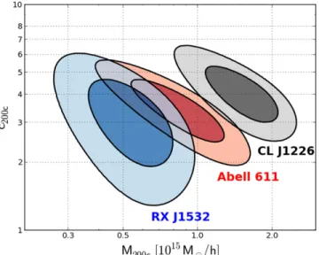
Table7. To visualize degeneracies and to show the information gain when including strong-lensing features into the recon-struction we explore the likelihood in the c–M plane for three CLASH clusters in Figure7.
4.4. Sources of Systematic Error
Before moving on in our analysis we want to discuss possible sources of systematic error. In the strong-lensing regime there is the possibility of false identification of multiple-image systems. In the case of CLASH, many strong-lensing features have no spectroscopic confirmation. However, CLASH can rely on 16-band HST photometry for photo-z determination. Finally, those systems which are only identified as candidates by the Zitrin et al. (2009) method for image identification are considered as such in our extensive bootstrap approach. Another problem for strong lensing is the shift of multiple-image positions by contributions of projected large scale structure. This has been pointed out recently in D’Aloisio & Natarajan (2011), Host (2012). However, as it was shown by the latter authors, the expected shift in image postion is well below our minimum reconstruction pixel scale of 5″–10″ for the different clusters(compare Figure2).
We address shape scatter in the weak-lensing catalogs with the adaptive-averaging approach of theSawLens method and by bootstrapping the weak-lensing input. Foreground contam-ination of the shear catalogs is another serious concern which will lead to a significant dilution of the weak lensing signal. In the HST images this is controlled by reliable photometric redshifts. However, there is the possibility of remaining contamination by cluster members in the crowded fields and by stars falsely identified as galaxies. Background selection in the ground-based catalogs is more difficult due to the smaller number of photometric bands. Hence, we use the Medezinski et al. (2010) method of background selection in color–color space which was optimized to avoid weak lensing dilution.
The aforementioned mass-sheet degeneracy(Equation (11)) is another concern for systematic error. We described the way of breaking this degeneracy in this work and tested the validity of this approach against numerical simulations (Merten et al. 2009; Meneghetti et al. 2010b). However, these simulations represent a much smaller sample and derive from a different selection function than the CLASH sample. Furthermore, the box-sizes of these cluster re-simulations is limited and therefore these tests do not guarantee that our treatment of the mass-sheet degeneracy produces fully unbiased mass estimates.
We have not commented yet on the dominant density peak in the lensing reconstruction as our center choice for the radial density profile. Because of the inclusion of strong lensing constraints, this peak position has an uncertainty of only a few arcsec(e.g., Bradač et al. 2006; Merten et al. 2011), but one might argue that e.g., the position of the clusterʼs BCG is a more accurate tracer of the potential minimum. However, our pixel resolution is of the order of∼5″ and BCG position and the peak in the surface-mass density coincide or are offset by one or two pixels.
More important is the effect of uncorrelated large scale structure(e.g., Hoekstra et al.2011, and references therein) and tri-axial halo shape(Becker & Kravtsov2011) which is picked up by our lensing reconstruction. Becker & Kravtsov (2011) claim that these effects introduce only small biases in the mass determination but increase the scatter by up to 20% with tri-axial shape being the dominant component. We do not seek to correct for these effects directly but adapt our way of analyzing numerical simulations accordingly (Section 6). In order to quantify our total error budget, we refer to Meneghetti et al.
(2010b) where our SaWLens approach of mass-modeling
underwent a thorough testing procedure in a controlled, simulated environment. Based on these results we report a systematic error between 5%–10%, depending on the level of substructure in the halo of interest.
4.5. Comparison to Other Analyses
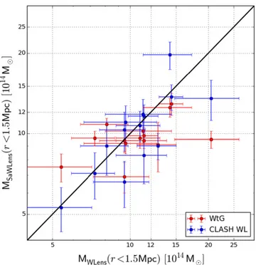
As afinal consistency check we look into 15 clusters that we have in common with the Weighing the Giants (dubbed as WtG hereafter) project (Applegate et al. 2014; Kelly et al. 2014; von der Linden et al. 2014) and the 16 clusters we have in common with the CLASH shear and magnification study by Umetsu et al.(2014; dubbed as U14 hereafer). For the direct comparison to WtG and U14 we calculate the enclosed mass within 1.5 Mpc of the cluster center following Applegate et al. (2014). This is to have a meaningful comparison at a fixed phyiscal radius and not to have to correct for the different mass apertures. We also used the cosmology of WtG to derive the masses for this comparison and show the mass comparison for the three data sets in Figure8. Wefind median values for the ratios MSaWLensMWtG and MWtG MSaWLensof 0.88 0.06
0.10 − + and
1.12−+0.100.06, respectively. The upper and lower bounds derive
from the third and first quartile of the ratio sample. For the unweighted geometric mean36 of these ratios we find 0.94± 0.11. The respective numbers for the 16 cluster comparison to U14 are 0.93 0.09
0.14 − + and 1.08 0.14 0.11 − +
for the median of the ratios MSaWLens MU14and MU14 MSaWLens. The geometric
mean of the ratios yields 0.95± 0.06. Although we see Figure 7. Likelihood of NFW fits in the c–M plane. The cluster Abell 611
represents a typical CLASH cluster at an intermediate redshift with the full set of lensing constraints available. RX J1532 is the only cluster in this c–M analysis without strong lensing constraints and CL J1226 is the only cluster in the sample without available Subaru weak lensing data. The inner and outer contours show the 68% and 95% confidence levels.
36The geometric mean satisfies X Y〈 〉 =1〈Y X〉 for the ratio of samples X and Y.
significant scatter between the different studies, there is general agreement but we have to point out that our analysis and U14 use identical Subaru weak-lensing catalogs. In the following subsections we report these different mass estimates cluster by cluster and also consult other studies of a specific object.
For a comparison of our mass estimates to X-ray masses we want to refer to the recent work by Donahue et al. (2014), where X-ray mass profiles from Chandra and XMM-Newton were compared to the lensing-derived profiles of U14 and to our profiles reported in Table6. Donahue et al.(2014) find that Chandra masses at 0.5 Mpc, assuming hydrostatic equilibrium, are on average 11% larger than the masses presented in this work for a sample of 10 clusters that the studies have in common. For hydrostatic masses from XMM-Newton at 0.5 Mpc, the opposite trend was found, where for a sample of 13 common clusters our lensing masses were 18% higher than the X-ray masses.
4.5.1. Abell 383
This cluster at z =0.188is one of thefirst clusters studied by CLASH Zitrin et al.(2011). In the mass comparison with WtG, our value of M1.5Mpc=9.6±0.6 × 10¹⁴M⊙ is larger than M1.5Mpc=7.3± 1.4 × 10¹⁴M⊙ of WtG at the ∼1.5σ level,
which is consistent with the findings of U14 with M1.5 Mpc= 7.1±1.4 × 10¹⁴M⊙. To have another
indepen-dent study we refer to Newman et al. (2013) who find
M1.7Mpc=6.6−+1.11.5×1014M⊙ for this object. The mass from
our model at the same radius yields M1.7 Mpc=
M 10.7±0.7×10¹⁴
⊙, which is again in some tension. The
reason for this discrepancy is unclear, especially since Abell 383 is thought to be a rather relaxed object. However, the tension is also not very significant.
4.5.2. Abell 209
Our lensing reconstruction of this system at z= 0.206 suggests a rather massive but regular system with respect to the morphology in its surface-mass density map. This is supported by our derived mass of M1.5Mpc =9.8±
M
0.7×10¹⁴ ⊙, which compares well to the findings of U14
with M1.5Mpc=11.6± 1.2×10¹⁴M⊙ and WtG with M1.5Mpc=
11.3± 1.5×10¹⁴M
⊙. An earlier study by Paulin-Henriksson
et al. (2007) reports M1.8Mpc 7.7 2.7 10 M 4.3 14
= − ×
+
⊙ and we
compare to our result at the same radius and using the same cosmology of M1.8Mpc= 11.7±0.9×10¹⁴M⊙, which shows
no significant tension but a higher mass. We would expect such a result since the background selection of weak-lensing galaxies in Paulin-Henriksson et al. (2007) was based on single-band data which is plagued by severe dilution effects (Medezinski et al.2007,2008).
4.5.3. Abell 2261
Abell 2261 at z=0.225 is one of the most massive clusters in our sample with one of the largest BCGs observed (Postman et al. 2012b). Our mass estimate of
M1.5Mpc=12.9±1.2×10¹⁴M⊙ is in excellent agreement with M1.5Mpc=13.7± 1.5×10¹⁴M⊙by U14 and M1.5Mpc =14.4±
M 1.5×10¹⁴
⊙by WtG. An earlier CLASH study by Coe et al.
(2012) derived a virial mass of Mvir 22.12.3 10 M 2.5 14
= + × ⊙,
which compares well to our virial mass estimate of Mvir=25.1±2.5×10¹⁴M⊙.
4.5.4. RXJ 2129
This low-mass system at z=0.234shows some interesting morphology in the surface-mass density map of its core (see Figure15). Since our fitting range starts at smaller radii, this might explain why our mass of M1.5Mpc=7.5± 0.9×10¹⁴M⊙
is larger, although insignificantly, than M1.5Mpc =5.4± M
1.7×10¹⁴
⊙ by WtG and shows some more tension with M1.5Mpc=5.3±1.0×10¹⁴M⊙by U14.
4.5.5. Abell 611
Also Abell 611 at z=0.288was studied by Newman et al. (2013) where a mass of M1.76Mpc=8.3−+1.21.5 ×1014M⊙ is
reported. At this radius we find M1.76Mpc=10.9± M
1.1×10¹⁴
⊙, in good agreement with this former study,
and also our value of M1.5Mpc=9.4±0.9×10¹⁴M⊙ is in
agreement with M1.5Mpc= 9.5±1.9×10¹⁴M⊙by WtG. This
picture is further confirmed by U14 with M1.5Mpc= M
10.3± 1.7×10¹⁴ ⊙.
4.5.6. MS 2137
MS 2137 is a well-studied cluster at z= 0.313for which we find a rather high mass of M1.5Mpc= 10.8±0.6×10¹⁴M⊙,
compared to M1.5Mpc=8.1±1.7×10¹⁴M⊙ by WtG and M1.5Mpc=9.0±2.0×10¹⁴M⊙ by U14. Also Newman et al.
(2013) looked at this system and found M1.32Mpc= M
3.6 0.8 10
1.3× 14 −
+
⊙. For this aperture however, we find
Figure 8. Comparison between our analysis and other weak-lensing studies. The red data points show clusters in common with WtG and the blue data points show the overlap with Umetsu et al.(2014). On the y-axis we plot
enclosedSaWLens masses within a radius of 1.5Mpc from the cluster center. The x-axis shows equivalent masses from WtG and U14, respectively. The black line indicates a one-to-one agreement.